Ground Penetrating Radar of Neotectonic Folds and Faults in South-Central Australia: Evolution of the Shallow Geophysical Structure of Fault-Propagation Folds with Increasing Strain

Abstract

Using ground penetrating radar (GPR) we investigate the near surface (~0–10 m depth) geophysical structure of neotectonic fault-propagation folds and thrust faults in south-central Australia in varying stages of fold and fault growth. Variations in neotectonic fold scarp heights are interpreted to reflect variations in accumulated slip on the underlying reverse faults. Fold scarps on the Nullarbor and Roe Plains are characterized by broad, asymmetric morphologies with vertical displacements of ~5 to ~40 m distributed over 1 to 2 km widths (~0.5 to ~4 m per 100 m). Within increasing scarp height there is an increase in the frequency and spatial density of strong reflector packages in the hanging wall that are attributed to material contrasts imposed by co-seismic fracturing and associated lithological and weathering variations. No evidence for discrete faulting is found at scarp heights up to 40 m (maximum relief of 4 m per 100 m). Where the principal slip zone of a fault ruptures to the surface, scarp morphologies are characterized by steep gradients (ca. 10 m per 100 m). Discrete faulting is imaged in GPR as structural lineaments, abrupt changes in the thickness of reflector packages with variations of amplitude, and/or hyperbolic diffraction packages indicative of the disturbance of reflector packages. Geophysical imaging of subtle changes in the shallow geological structure during growth of fault-propagation folds can be conducted using GPR informing the identification of locations for invasive investigations (e.g., trenching).

1. Introduction

The surface manifestations of faulting can vary significantly, depending on the characteristics of faulting (e.g., fault kinematics, geometry, slip) (e.g., [1,2,3]) and the geological and material properties of the faulted medium (e.g., [4,5]). Incipient, structurally immature, and/or slow slip rate intraplate faults may develop wider fault zones by distributing more energy into small-scale fracturing and frictional processes relative to interplate faults (e.g., [6]). Geophysical and field observations of cumulative slip indicate that up to two thirds of strain on thrust faults may be accommodated by distributed folding [7,8]. The same can be seen at the scale of individual earthquakes; the Chi-Chi [9] El Asnam (e.g., [10,11]) and Peterman Ranges earthquakes, for instance, all displayed distributed deformation at scales of 10 to >1000 times the vertical displacement. The presence of strong horizontal layering, material property contrasts and less cohesive near-surface materials may encourage distributed deformation that is greatly in excess of the displacement localized at the principal slip zone (e.g., [12,13,14,15,16,17,18,19]).

Understanding the spatial distributions of deformation in evolving fault zones has important implications for seismic hazard analysis, such as probabilistic fault displacement analysis [20,21,22,23].

In Australia, around 2900 individual surface traces sum to around 350 neotectonic surface features (faults and folds) that are attributed primarily to reverse-faulting within a regional compressive stress field [24]. Our work ([25], this study) builds on previous studies of the Nullarbor and Roe Plains (e.g., [26]) to show that approximately 300 neotectonic fold scarps displace the Eocene—Miocene limestones of these vast limestone plains alone (Figure 1B and Figure 2). A further ~80 neotectonic scarps are located in South Australia. Combined with the Nullarbor scarps, this accounts for ~13% of Australia’s known neotectonic scarps. Their surface morphologies range from folds to monoclines to discrete surface faulting (e.g., [24]). Their surficial geology ranges from generally flat-lying Neogene limestones of the Nullarbor and Roe Plains (e.g., [26]) to bedrock-gravel contrasts across South Australian Faults (e.g., [27,28,29]). These contrasting properties, including morphology, geology, and structural maturity, offer an opportunity to explore the utility of ground penetrating radar (GPR) to investigate the distribution of cumulative surface deformation across a typical range of Australian Faults.

The Nullarbor and Roe Plain exhibit scarps with broad morphologies (e.g., 30–40 m height over distances of 1–2 km) that lack evidence for discrete strain localization (e.g., fault rupture traces) and are thus referred to as fold scarps (e.g., [25]). In contrast, neotectonic faults include ≥ 100 m high scarps with steep gradients (e.g., 10 m relief/100 m wavelength such as the Willunga and Wilkatana faults in South Australia [27] and ca. 1 to ~10 m high scarps produced by discrete surface ruptures during historical events (e.g., [30]. Simplistically, fault-propagation folds are considered to represent incipient phases of fault growth that progresses to increased folding and fracturing of near surface materials and eventually to surface rupture as upward tip of the principal slip zone breaches the surface.

GPR is commonly used to investigate neotectonic faults in seismically active regions (e.g., [8,31,32]). In contrast, only a few Australian neotectonic scarps (e.g., Meckering, Hyden, Dumbleyung, Cadell) have been studied using geophysical imaging methods such as GPR or seismic reflection surveys (e.g., [33,34]). Although the quality of interpretable data is highly dependent on the physical properties of the subsurface materials these non-invasive methods have provided promising results that encourage future application in the investigation of neotectonic structures in Australia.

In this study, we use GPR to image shallow (ca. 0–10 m depth) fault structure across a selection of faults on the Nullarbor and Roe Plains (Figure 1B and Figure 2) and the Willunga Fault scarp (Figure 1C–E) in the Mount Lofty Ranges. This represents a geologically diverse array of faults with substantive variations in total neotectonic slip, on which to characterise the structural evolution of faulted sedimentary rocks during fault growth. We aim to diagnose neotectonic structural and sedimentological features in the GPR that provide insights into the evolution of near surface features with progressive strain. This can provide implications for the associated distributed deformation and, by extension, the fault displacement hazard in the affected area.

1.1. Geology

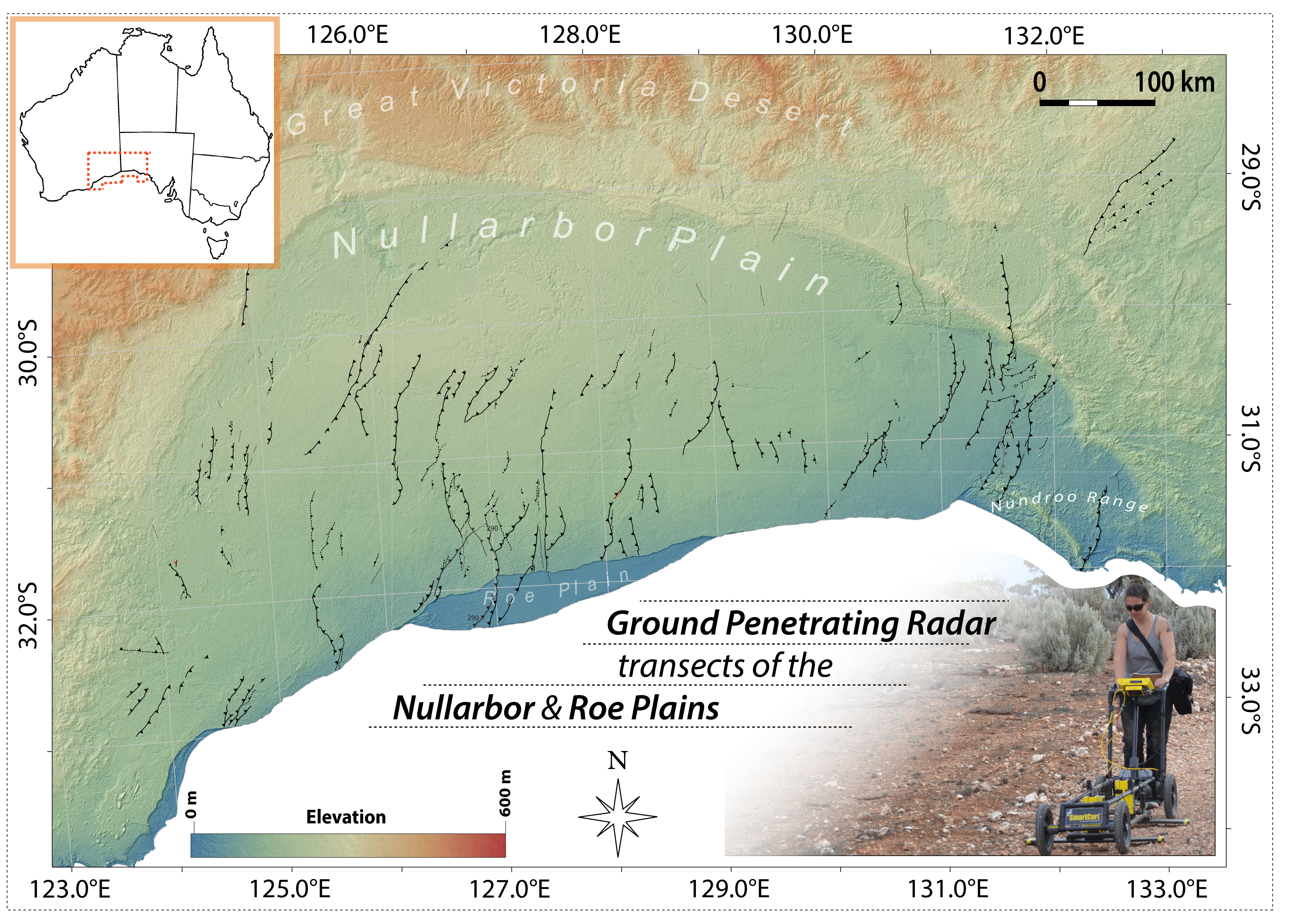
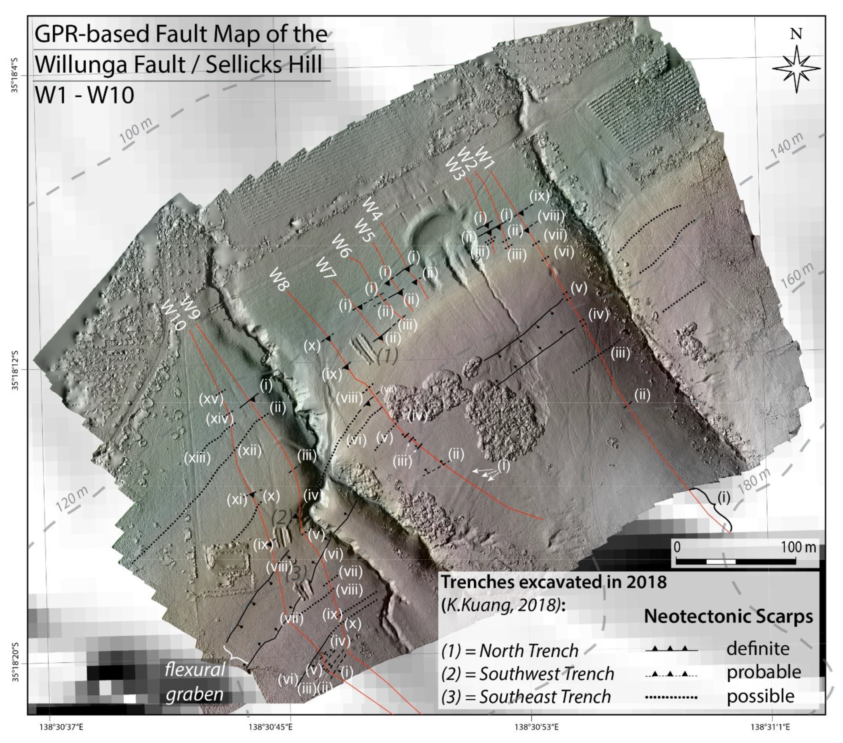
1.1.1. Willunga Fault

For a detailed description of the geological setting of the Willunga Fault site we refer the interested reader to, e.g., [35,36]. The Willunga Fault is one of several reverse faults bounding the Mount Lofty Ranges to the East and West within proximity to Adelaide (<50 km)(Figure 1C–E) thrusting Proterozoic and/or Cambrian basement rocks over Quaternary sediments (e.g., [28,37,38]). At the study site in Sellicks Hill, SA, these are in particular Cambrian Heatherdale Shale, that consist of pyritic, calcareous shale and siltstones [39] and Quaternary clay-rich colluvial sediments which have been observed in trenches excavated during field campaigns in 2018 [18,40] and 2022 [41].

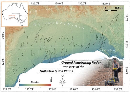
1.1.2. Nullarbor & Roe Plains

The limestones of the Nullarbor and Roe Plain are underlain by Precambrian rocks dissected by N to NE shear zones and faults imaged in magnetic, gravity and deep crustal seismic reflection data [42,43,44,45]. Many of these structures have been reactivated in the neotectonic regime (e.g., [46]). The basement rocks are overlain by up to 300 m thick Cretaceous sandstones and shales [47] that were deposited in a terrestrial to lacustrine/marine environment along Australia’s evolving passive continental margin during the rift phase associated with the separation of Antarctica and Australia [48]. The establishment of fully marine conditions and carbonate sedimentation along the southern coast resulted in the deposition of the Eocene-Miocene Eucla-Basin limestone successions [26,49,50] which are divided into three main units, distinguished by unconformities that developed throughout sea-level low stands. The up to 300 m thick middle-late Eocene Wilson Bluff Limestone is the oldest and thickest unit, followed by the late Oligocene to early Miocene Abrakurrie Limestone, up to 100 m thick, and the middle Miocene Nullarbor Limestone, ca. 20–30 m thick [51,52,53].

2. Data and Methods

2.1. Digital Elevation Models (DEM’s)

Geomorphic mapping of fold scarps on the Nullarbor and Roe Plains was conducted using 12-m resolution TanDEM-X [54] and 30- & 90-m Shuttle Radar Mission (SRTM) data [55] in ArcMap (Figure 1B) [17]. For the Sellicks Hill site of the Willunga Fault a 10 cm DEM was available generated from drone photogrammetry using AgiSoft Photoscan (from [18]; Figure 1E) (e.g., [56,57,58,59]). Analysis of the Willunga Fault DEM reveals numerous fault traces at the surface (Figure 1E and Figure 2) that were confirmed as Quaternary ground surface fault ruptures in subsequent excavations [18,41].

2.2. Ground Penetrating Radar (GPR)

GPR employs electromagnetic (EM) waves, typically in the range of 10 to 1000 MHz. These are emitted into the ground from a transmitting antenna, reflected where the dielectric permittivity of the subsurface changes (e.g., [60,61]). Generally, the higher the employed frequency of the signal the higher the resolution of the imaged reflectors, however, the lower the penetration depth. The technique has several limitations to its utility. Some of these are universal and commonly reported from GPR studies of active faults (e.g., [62,63]) paleoseismic faults (e.g., [32,34,64]) and folds (e.g., [65]) in diverse settings. For example, electrically conductive materials like clay-rich and moist soils/sediments attenuate the radar signal while dry massive rock layers or sandy sediments are less conductive and so allow deeper penetration. Embedded boulders, cobbles, tree roots and other objects can scatter and obscure the signal, and may be imaged as arcuate, i.e., hyperbolic diffractions. These general factors mean that the quality of the GPR data, including penetration depth, is highly dependent on the local geology. Additional factors that can influence GPR signal depth and interpretability include the extent and mineralogy of the weathered zone, climatic conditions that allow deep weathering of colluvial deposits, and the degree of bioturbation.

Twelve GPR transects with total lengths of 109 to 1160 m were conducted across 5 fold scarps on the Nullarbor and Roe Plain and ten transects of lengths of 72 to 380 m across the Willunga Fault south of Adelaide (Figure 1 and Figure 2). The scarps were selected to represent examples of relatively low, moderate, and high displacements.

All GPR data sets were collected using a Sensors and Software pulseEKKO PRO GPR unit and antennas with frequencies of 100 and 200 MHz. Traces were recorded at 0.25 and 0.1 m intervals, respectively (antenna frequencies, trace intervals, time window, and number of stacks for each transect are listed in Table S1 in the Supplementary Material). Each transect was tracked using Avenza Maps and start and end points were additionally recorded with a handheld GPS unit. The GPR data was processed in ReflexW using the Move Starttime, Subtract-Mean (Dewow), Energy Decay, Bandpass Butterworth, Background Removal and Correct 3D Topography Filters. The data was then exported as image files in a variety of colour schemes and with and without topography applied for interpretation in ReflexW 2D.

A frequency of 100 MHz was chosen for both sites based on the best expected penetration/resolution ratio; i.e., we aimed to increase penetration depth while providing sufficient resolution to image secondary, coseismic deformation features like fissures and cracks in the limestones of the Nullarbor and Roe Plain, and to capture deeper features at the Willunga site. In addition, 200 MHz antennas were employed at the Willunga site to increase resolution of near surface features.

Many of the Nullarbor GPR transects are heavily impacted by vegetation, wombat burrows and karst features, such as cavities, causing scattering and diffractions in the EM signal. Anthropogenic effects are minimal. Routes for the GPR cart were kept as straight as possible and perpendicular to fold-fault traces. On the Nullarbor we attempted to locate the transects between at least the highest point of the scarp and past the transition between the scarp slope and the footwall. In case of lines N8, N9, N10, N11 and N12 (see Section 3) this was difficult to achieve due to extremely uneven ground conditions with numerous wombat burrows, surface karst features and vegetation. These transects cover the slope of the mapped fold scarps. The scarp slope at the Willung lines W2–W7 was too steep to safely traverse with the GPR cart.

The local surface geology in the Nullarbor and Roe Plain study area varies across the GPR transects.

Lines N1 and N2 were conducted on the central Nullarbor. The imaged lithology is Nullarbor limestone overlain by variably thick regolith with local calcretezation. Line N3 is located on the Roe Plain in ~2 m thick Roe Calcarenite that unconformably overlies the Abrakurrie and locally the Wilson Bluff Limestones [66]. Line N12 was conducted at the northern tip of a fold scarp that terminates at the inland boundary of the Nullarbor, the Eocene and Miocene shorelines which are draped by Quaternary, active dune fields. Here, the Nullarbor limestones are overlain by undifferentiated Tertiary to Pleistocene karst-related sediments and undifferentiated Quaternary aeolian sediments [67].

All other lines were conducted across the easternmost mapped fold scarp along which the surface geology transitions from the Pleistocene Bridgewater Formation which is defined as ‘bioclastic barrier shoreline deposits, silica rich, with heavy minerals, shallow subtidal; Coastal, cross-bedded aeolian calcarenite with palaeosol horizons and capped by calcrete’ [68], towards Pleistocene carbonaceous gravels, clay silts and sands overlying nodular/tabular calcrete and calcareous, partially aeolian silts to fine sands [69].

Additionally, dayas, collapse dolines, ponding features along fold scarps and other karstic or denudation features usually provide favourable, localised conditions for sediment deposition (e.g., [70]). These deposits contain reddish clay-rich silts and sands from wind-blown sources (e.g., [70]) and can be several metres thick as evidenced by several augerholes drilled into ponding features at the base of fold scarps (e.g., Figure 5A).

In summary, the geology across our sites varies for both faulting and non-faulting related reasons, and the age of the faulted materials in the Nullarbor Plain (ca. 3 to 10 Ma) varies substantially from those at the Willunga Fault (Neoproterozoic to Late Quaternary).

3. Results

3.1. Willunga Fault

Structural interpretations of the GPR data are based on the 200 MHz data because these are imaged at a higher resolution and the lower 8 m of the 100 MHz data was sufficiently noisy to preclude derivation of any additional information at depths below the 200 MHz limits. The Willunga transects are generally characterized by a variably disturbed, strong reflector package at the surface of up to ~2 m thickness with a relatively well-defined boundary at depth (i.e., maximum penetration depth) beyond which the EM signal is attenuated and only background noise is recorded. Despite large amounts of clay in the near surface sediments, the depth of penetration achieved at the Willunga site captures most of the features that have previously and recently been mapped and observed in excavated trenches and existing gullies (Figure 1 and Figure 3; [18,40,41]). Additionally, the GPR data has captured several features that may represent sub-structures within larger structures, such as half-grabens in a flexural graben on the hanging wall (e.g., Figure 4C, S10).

In the following the most prominent features are described, visible in the topography and DEM and those that have been interpreted from excavations in 2018 [18,40] and more recently in May 2022 [41]. For detailed interpretations of all transects we refer to the Supplementary Material. Before and during the 2018 excavations the assumed main reverse fault at the bottom of the steepest section of the scarp was observed in the north-easternmost gully above the dam and in trench (1) (Figure 3 and Figure 4A). Colinear features in the transects W2 and W6–10 (features (iii), (iii), (ii) (ix), (ii) and (xii), respectively) have been observed in the GPR data. Evidence for at least two other faulting-related features further downslope is interpreted from the GPR data along all transects (Figure 3), the topography and the N-trench of the 2022 trenching-campaign [41].

The reverse fault observed in trench (2) is imaged in lines W9 and W10 (features (iv) and (ix), respectively; Figure 4B, Figures S9 and S10). The strike of the fault between trench (2) and its location along transect W8 appears to correlate with the orientation of the kinked, SW-NE running creek section. It is not clear whether feature (vi) or (vii) along W8 represent the extension of the reverse fault on the NE side of the creek.

A prominent hanging wall feature, an up to ~36 m wide flexural graben interrupted by the creek, is obvious in the DEM and in the field (Figure 3 and Figure 4C). The graben shoulders are imaged in the GPR data along line W1 by feature (v) and (iv), and along W9–W10 by features (v)/(iv) and (vii)/(viii), respectively. The SE shoulder was observed in trench (3) during the 2018 campaign (Figure 4C), and the southern trench of the 2022 campaign exposed the NW shoulder [41]. In the three transects that crosscut the graben the GPR data appears to image further horst and graben sub-structures, indicated by changes in reflector package thickness, disrupted reflectors and hyperbolas (Figure 4C, trench (3) and Figures S1, S9 and S10).

Based on previous field mapping and paleoseismic trenching at the same site across the Willunga Fault as the GPR transects we assume the maximum penetration depth to coincide with the boundary between the unconsolidated Quaternary sediments and the siltstones and shales of the basement. Furthermore, we were able to interpret and verify observed features in the GPR data where these spatially correlate with observed surface features and features in the trenches.

These features include:

➢

Interrupted/Offset reflectors in transects without topography. These can aid in the identification of the same feature in the respective transect with superimposed topography (see, e.g., Figure S4, line W4). Transects that have not been corrected for topography are vertically exaggerated and can highlight features imaged in the GPR data that correlate with real features and may not be as obvious in the corrected data.

➢

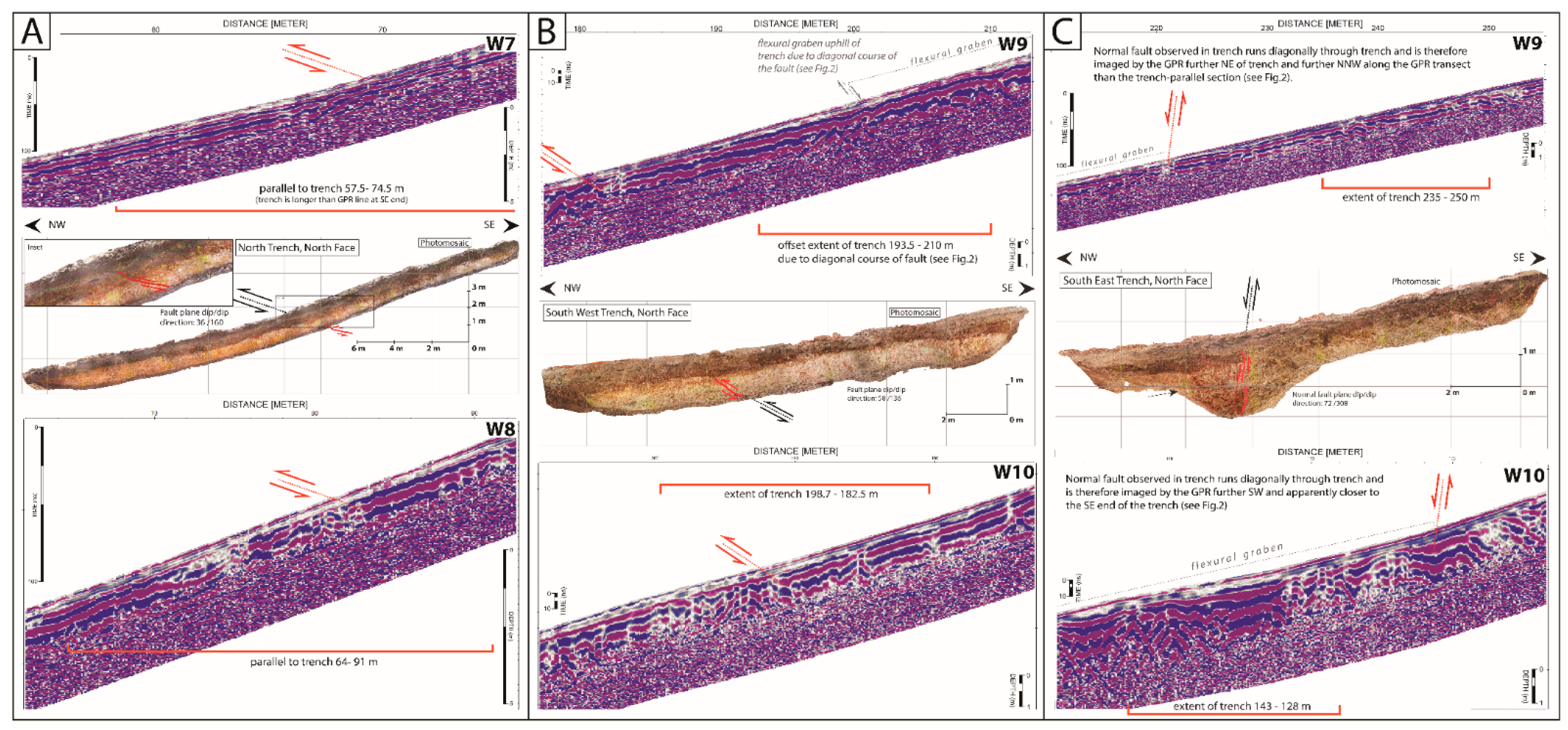
Thickening/Thinning of reflector packages is interpreted to indicate locations of faulting. Reverse faulting offsets the bedrock and overlying sediments relative to each other along the fault plane, forming an uplifted hanging wall and a downthrown footwall and increasing the erosion rate on the hanging wall (e.g., Figure 4B, W9). Initially, unstable sediment on the newly developed scarp crest erodes and is deposited at the bottom of the scarp on the footwall as colluvium. Further erosion and degradation of the scarp results in further colluvial sedimentation on the footwall, increasing sediment thickness above the basement rocks and decreasing thickness on the hanging wall. Thickening/thinning of reflector packages is usually accompanied by hyperbolic shaped diffractions indicating the actual disturbance of the subsurface, i.e., fracturing and/or related reworking of material and associated diffraction point sources such as smaller boulders, gravel, or clumps of sediment.

➢

Depending on the spatial extent of the disturbance the occurring hyperbolas often overlap and obscure the causative structure, making it difficult to clearly identify, e.g., dip directions and hence kinematics without ground-truthing the feature (e.g., potential sub-structures in a flexural graben on the hanging wall in line W1, W9 and W10). These structures are therefore not included in the fault line map in Figure 3, however, indicated in the interpreted transects in the Supplementary Material.

Identified features along each transect are contiguously numbered with (i), (ii), (iii), etc., following the direction of data acquisition. Each feature was initially marked at its location along the transect and subsequently interpolated and/or connected with apparently colinear features identified along other transects or where they are visible in the DEM. The three confidence levels of definite, probable, and possible are assigned to each feature based on ‘clarity’ in the GPR data and additional ‘visibility’ in the DEM, i.e., the geomorphology, and/or in trenches:

➢

Definite—clearly identifiable in the GPR data due to, e.g., unambiguous thickness change in the reflector packages, and identifiable in the topography and/or a trench/outcrop.

➢

Probable—feature not unambiguously identifiable in the GPR data, e.g., due to being located within a zone of disturbed reflectors. However, additional geomorphic expression or collinearity with adjacent definite, probable, or possible surface features along transects or in trenches/outcrops.

➢

Possible—feature not unambiguously identifiable in the GPR data (see above) and no other evidence available or not identifiable in GPR data morphological expression with unknown origin, however, possibly colinear with other identified definite, probable, or possible surface features.

3.2. Nullarbor & Roe Plain

Due to the predominantly unconsolidated surface materials with various degrees of calcretization within the Bridgewater Formation the GPR transects of lines N4, N5, N6, N7 image sedimentary strata well and penetration depths reach up to ~8 m, indicated by a paleo-surface imaged in these transects. Overall, the other transects appear to reach similar penetration depths, however, the signal response is weaker, likely due to smaller contrast changes in the subsurface material, so that reflections and diffractions from non-geological sources, such as trees, metal objects, burrows, and background noise obscure the GPR data. Figures of the uninterpreted transects are provided in the Supplementary Material.

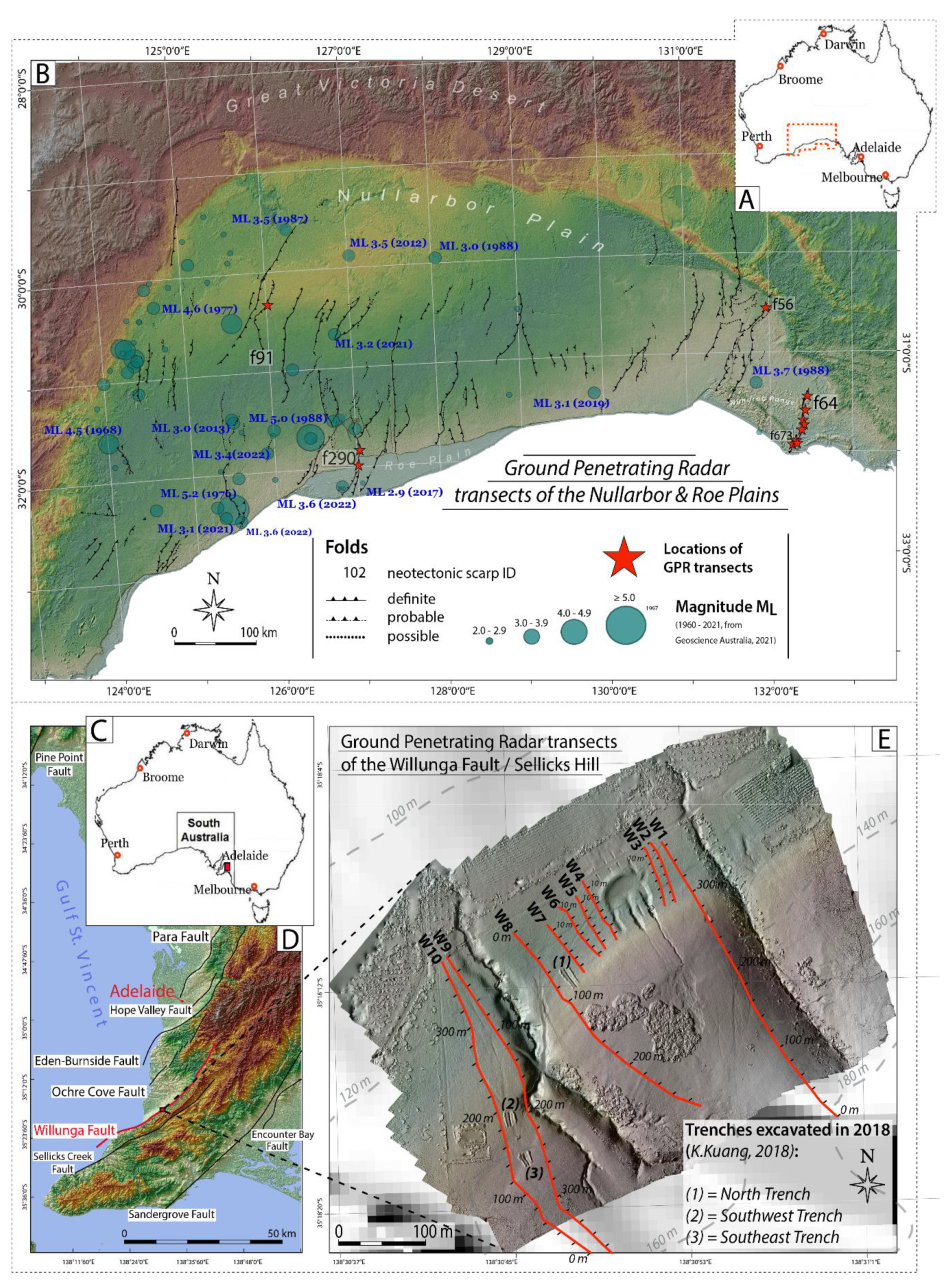
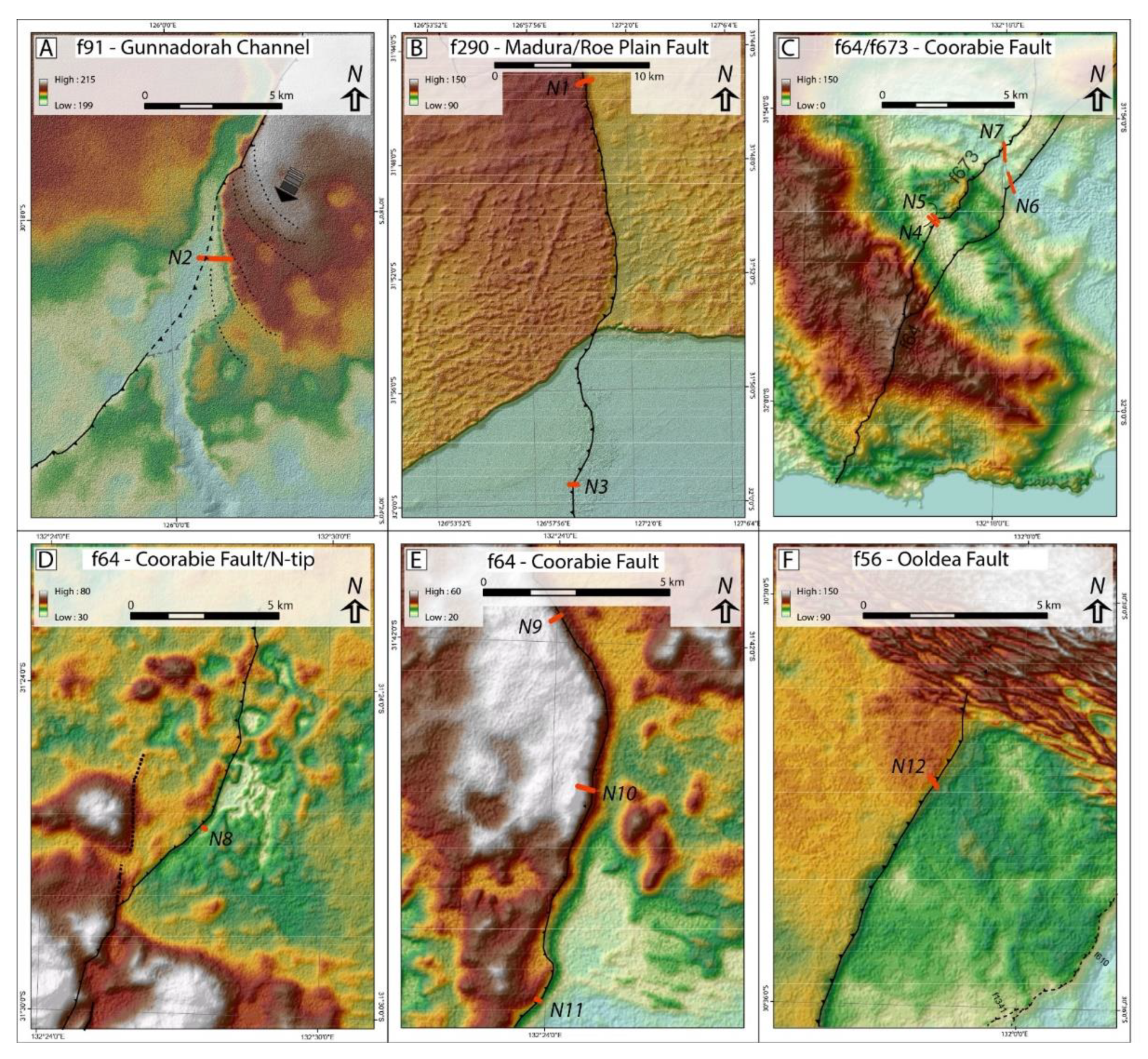
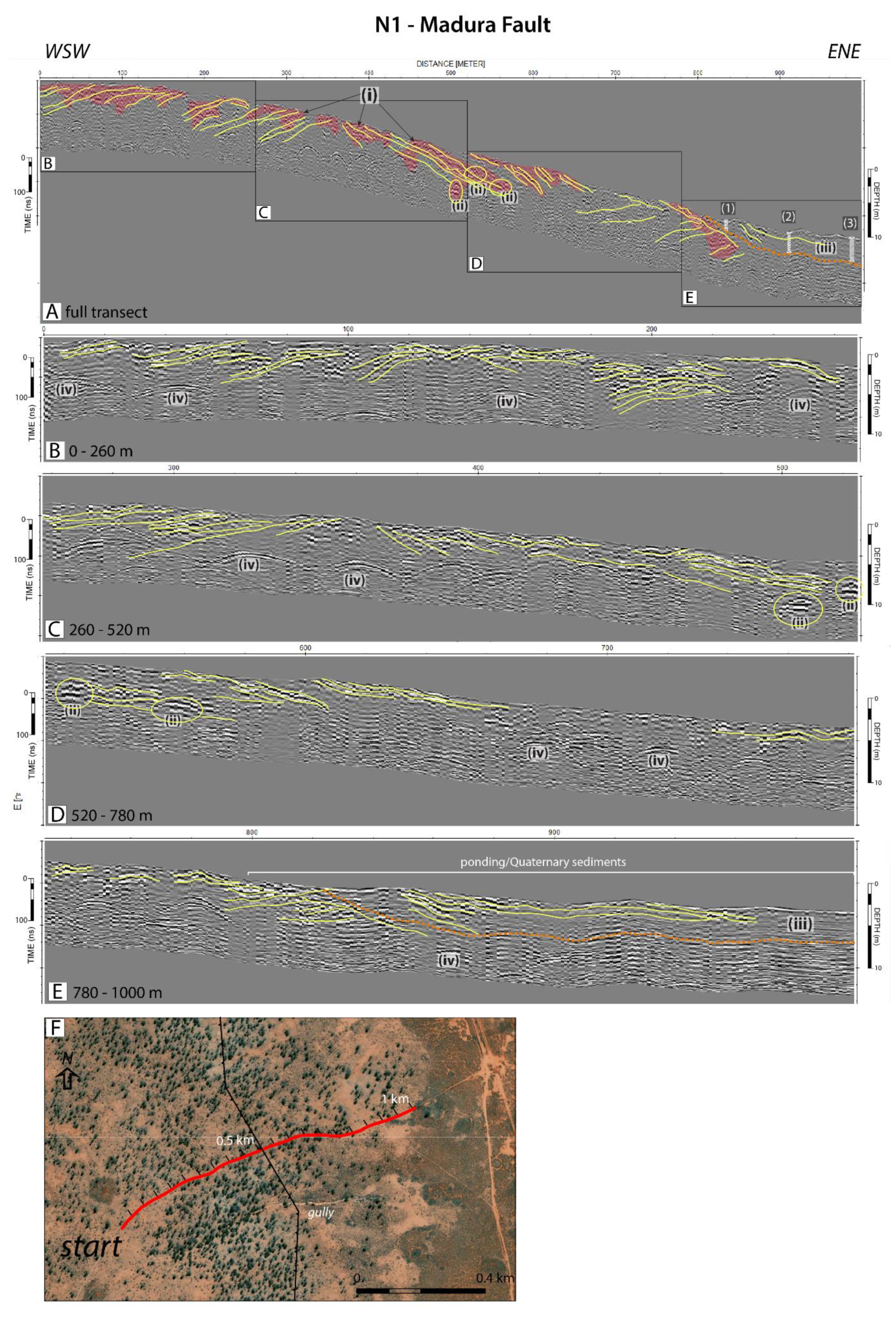
3.2.1. Line N1—Madura

The transect is located on the south-central Nullarbor, approximately 16 km north of Madura Roadhouse (Figure 2B). Numerous airwave reflections dominate the lower 5 m of the data (Figure 5, wide hyperbolas, feature (iii)) with mostly weak reflectors, however, a considerable number of reflectors (yellow, solid lines) dipping up-slope between 0–360 m and down-slope between ~380–600 m have been identified where stronger and deeper penetrating reflector packages occur. The interpreted reflectors are not parallel to the surface which may either imply that they represent the primary sedimentary strata, i.e., crossbedding of the limestones prior to scarp formation, or onlapping growth strata, i.e., the scarp was forming during deposition of the limestones. Because the interpreted reflectors ENE of the ~360 m mark consistently dip into the same direction as the scarp slope we interpret these to image onlapping sedimentation of carbonates during scarp formation.

The reflectors WSW of the ~360 m mark are, however, more likely to image crossbedding within the limestones. They dip into the opposite direction of the scarp surface and, assuming no topography, have a steeper dip angle in relation to the surface than the reflectors ENE. If they represented growth strata onlapping onto the hanging wall and therefore the shallower dipping backlimb of the scarp their dip would be expected to be shallower, too, compared to the ENE reflectors the ~360 m mark consistently dip into the same direction as the scarp slope we interpret these to image onlapping sedimentation of carbonates during scarp formation.

Some of the most pervasive reflectors between ~400–600 m spatially coincide with three hyperbolic shaped diffractions (feature (i)) with velocities identical to those of limestone, i.e., ~0.12 m/ns. These represent point sources within the limestone, such as fractures, minor narrow cavities, or discrete calcretization. Their depth provides a minimum measure of signal penetration of ~5 m. The section between ~800 m and the end of the transect (Figure 5E) correlates with a zone of sediment deposition at the base of the scarp where ponding occurs after rainfall events (zone (ii)). In zone (ii) above the orange, dashed line, reflectors appear parallel and undisturbed, and onlapping onto the scarp at their location of contact. The GPR-inferred thickness of these sediments, marked by the orange, dashed line, correlates roughly with maximum depths recorded from augerhole (3) (i.e., 2.92 m, Figure 5A). Towards the base of the scarp and where the scarp slope transitions into the ponding feature at ~600–840 m (Figure 5D,E) the angle of downslope-dipping reflectors becomes shallower and eventually dips the opposite direction. We interpret this to represent channelized sedimentation at the former base of the scarp in a seismically quiescent period. A few reflectors that lie below the interpreted base of Quaternary sediments (orange, dashed line) and unconformably overlying the channelized sediments are interpreted to represent continued onlapping sedimentation during renewed fold growth. Because the base of the Quaternary ponding sediments is inferred from augerholes, any reflectors above the orange dashed line are interpreted to represent strata within the ponding feature.

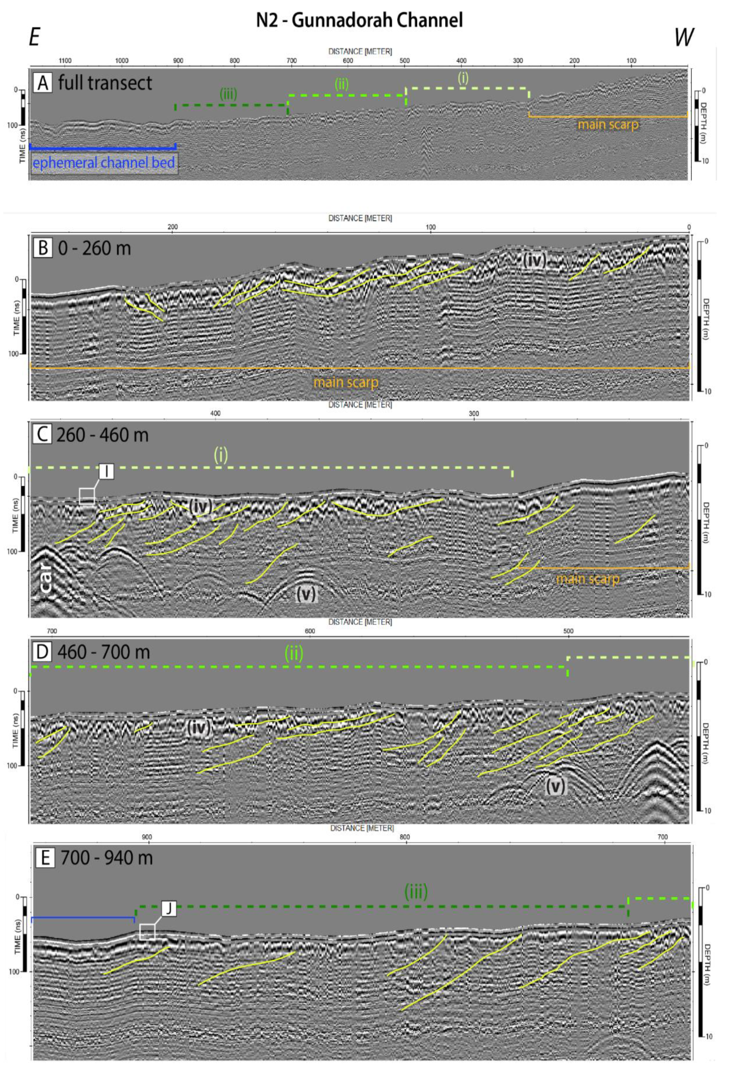
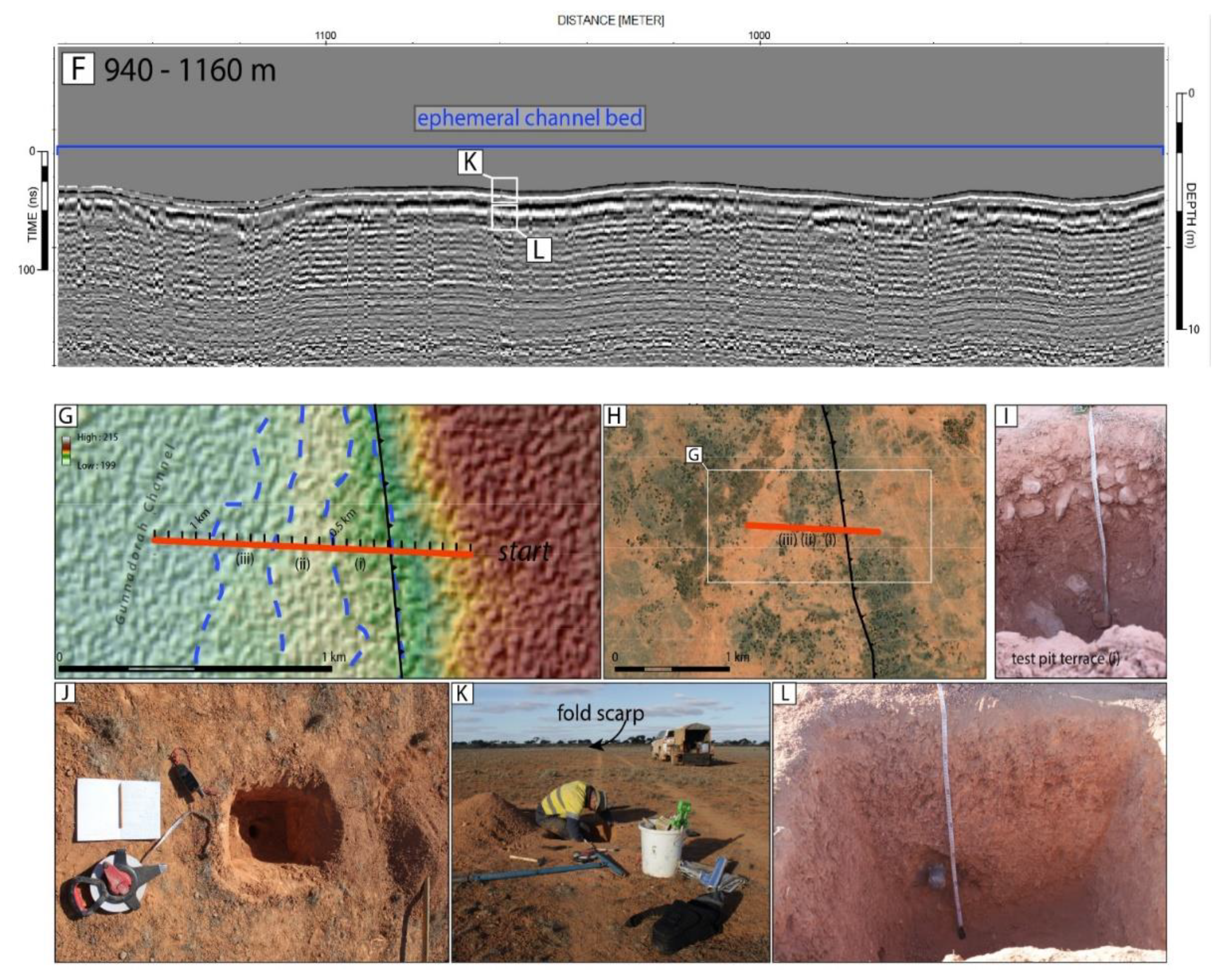
3.2.2. Line N2—Gunnadorah Channel

The GPR transect is located where the fold scarp of f91 interacts with the Gunnadorah Channel (Figure 2A), an ephemeral channel that can hold water along several km of its course after heavy rain events (pers. communication with local station owners), however, is assumed to have been most active during the Pliocene wetter climate ~5–3 Ma (e.g., [26]) providing implications for relative ages of scarp formation [17]. Progressive migration of the channel course towards the south driven by recurring vertical deformation along the interpreted causative fold line scarp (Figure 2A, grey dashed and solid line) is evidenced in the 12 m TanDEM-X data by preserved, curvilinear NNE paleochannel banks (Figure 2A black dashed lines). The channel eventually defeated the scarp and continues across towards the S-SSE (Figure 2A). Further deformation must have occurred while the channel was still active implied by three degradational terrace risers or possibly more recent fold scarps in the ponding area that formed before the channel was able to cut through the scarp (Figure 2A and Figure 6A). The GPR data and integrated topography, and a close-up of the DEM (Figure 6A–G) reflect these terrace risers (Figure 6A–E,G, (i), (ii) and (iii)), positioned between the present-day main scarp and the edge of the Gunnadorah Channel. Adjusting the colormap in the DEM to an elevation range of 199 to 215 m highlights these terraces in different colours of which the edges coincide with distinct elevation changes in the topography, at least at the transition from the main scarp to terrace (i) and terrace (i) to terrace (ii). The elevation change between terrace (ii) and (iii) is not as clear and at least two other locations within terrace (iii) indicate a similar elevation change at ~750 m and ~800 m. However, textural and thickness changes of the uppermost strong reflector packages in the GPR data also coincide with the interpreted boundaries between terrace (i), (ii) and (iii). I.e., the uppermost reflector package on the main scarp and all three terraces is highly disturbed by numerous hyperbolic diffractions, caused by nodular to tabular calcrete, with an exception of the lower section of the main scarp where the reflectors are nearly undisturbed (~220–280 m). Hyperbola size (i.e., length of hyperbola tails) decreases from the main scarp to the lowest terrace (iii). Similarly, thickness of the reflector package decreases from the main scarp (~2.3 m) towards terrace (iii) (~1 m). The channel bed between ~905 m to the end of the transect is imaged by a mostly undisturbed strong reflector package. We interpret the texture and thickness changes of the uppermost strong reflectors to represent different stages of calcrete development indicative of the relative ages of each surface with the main scarp being the oldest surface.

Within the terraces and the main scarp, a number of mostly down-slope dipping reflectors (Figure 6B–E, yellow lines) were identified which may represent sedimentary strata within the underlying limestone. Their dipping angles appear mostly steeper than the angle of reflectors within the upper 2–2.5 m, i.e., within the calcrete, which likely image fluvial sediment strata within the former channel bed during fold growth.

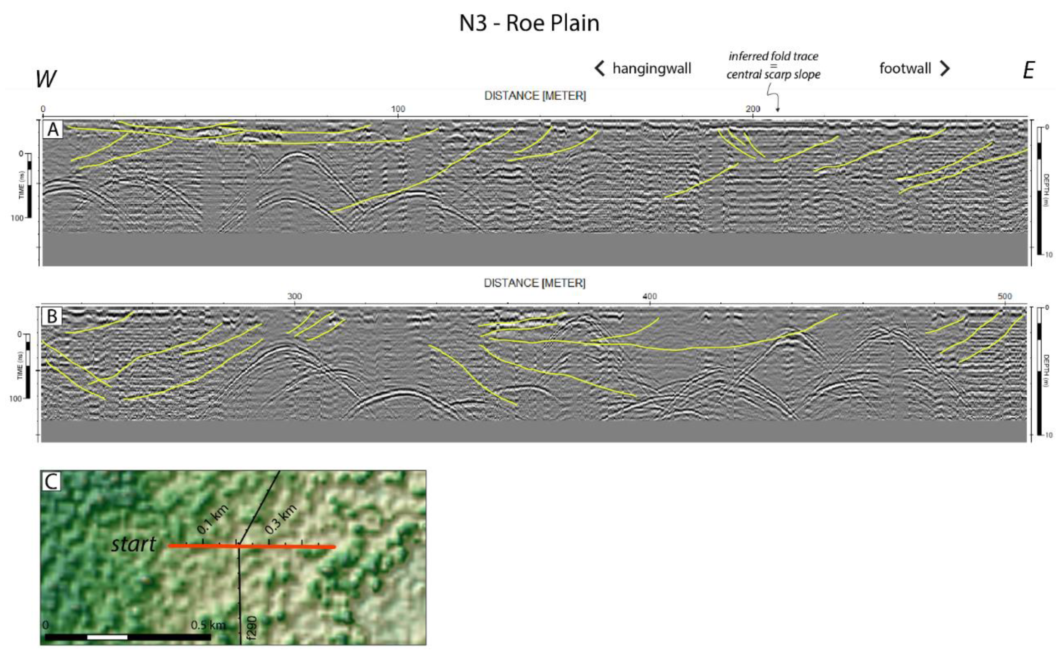
3.2.3. Line N3—Roe Plain

This transect crosses the same fold scarp as N1 but is located on the younger surface of the Pleistocene Roe Plain (Figure 2B and 7). Vegetation size and density increases in the proximity and along the scarp, so that the transect contains many hyperbolic diffractions originating from tree airwave reflections (Figure 7). Additionally, a fibre optic trench (discovered after the survey), numerous wombat burrows and perhaps karstic features are imaged by further hyperbolas. The DEM in this area was noisy in the zone of denser vegetation along the fault, so it was not possible to extract a reliable ground surface profile from the DEM. Although obvious on a vertically exaggerated DEM the scarp was not visible in the field, consistent with its very low gradient. We therefore used the GPR transect without adjusted topography for interpretation (Figure 7).

Several strong but discontinuous surface reflectors correlate roughly with reported thicknesses of the Roe Calcarenite (upper 1–3 m, Australian Stratigraphic Units Database, last accessed: 10 July 2022). The Roe Plain is eroded into the Abrakurrie Limestone which is likely to be represented by the main body of the GPR data below the stronger surface reflectors. Several inclined, often curvilinear reflectors (yellow solid lines) have been identified within the limestone, possibly imaging sedimentary strata. Although the density of interpreted reflectors does not allow a detailed picture of the limestone strata structure, varying dipping directions of interpreted reflectors imply localised erosion surfaces and channelization during deposition.

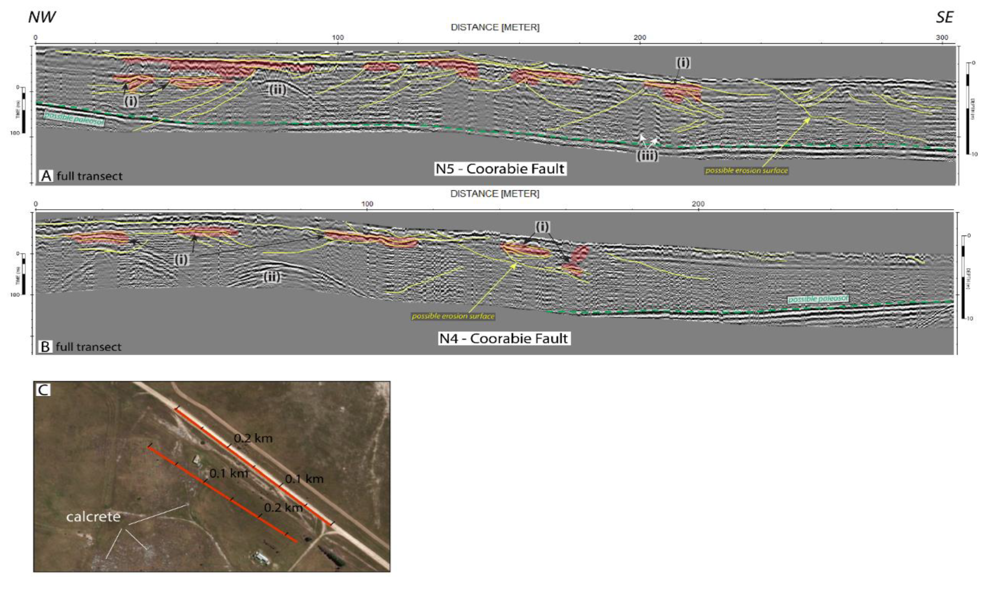
3.2.4. Line N4 & N5—Coorabie Fold—Wookata School

Both transects were conducted adjacent to the old Wookata School building, approximately 4 km southwest of Coorabie across a splay of f64. The Geological map of South Australia indicates both transects are situated within an elongated valley in the Pleistocene Bridgewater Formation. Fold f673 crosscuts the deposits in the valley which may be additionally draped by more recent, windblown coastal sediments.

Both transects display a strong, undisrupted reflector package at ~5.5–6 m depth (Figure 8, (green, dashed line) which we interpret to image a paleosurface within the Bridgewater Formation. No reference exposures of Bridgewater Formation deposits of thicknesses consistent with the depth of this reflector package were found in the field, however, the paleosurfaces are described to occur within the Formation in the Australian Stratigraphic Units Database (see Section 1.1.2) and a drilling campaign proximate to the GPR transects [71] reached drill hole depth of up to 18 m exposing only Bridgewater Formation. This implies that achieved penetration depths along the GPR transects purely image the deposits of the Bridgewater Formation.

The paleosurface is mostly unconformably overlain by a unit with weak reflectors often obscured by multiples and other reflections and diffractions (e.g., (ii) and (iii)). Strong airwave reflections image the school building at ~70 and ~80 m (feature (ii)). Inclined, curvilinear reflectors are likely imaging the cross-bedded, sedimentary structure of the Bridgewater Formation (solid, yellow lines below ~1–2.5 m), possibly imaging erosion surfaces and/or channelized deposition (Figure 8A,B). Strong, often discontinuous reflectors of the upper ~1–2.5 m characterize both transects at the surface, likely imaging developing calcrete (e.g., Figure 9D). In both transects the overall occurrence and depth of more localised, surface-parallel, strong reflector packages increases underneath the scarp slope and the hanging wall (features (i), reddish zones). These reflectors may represent locally calcretized paleosurfaces or progressed calcretization/cementation in elevated terrain due to favourable conditions for carbonate deposition. Along N4 the unit above the interpreted paleo-surface at depth thickens progressively from SE to NW, i.e., from underneath the footwall towards the hanging wall. The opposite occurs along N5, i.e., the top unit thins underneath the hanging wall.

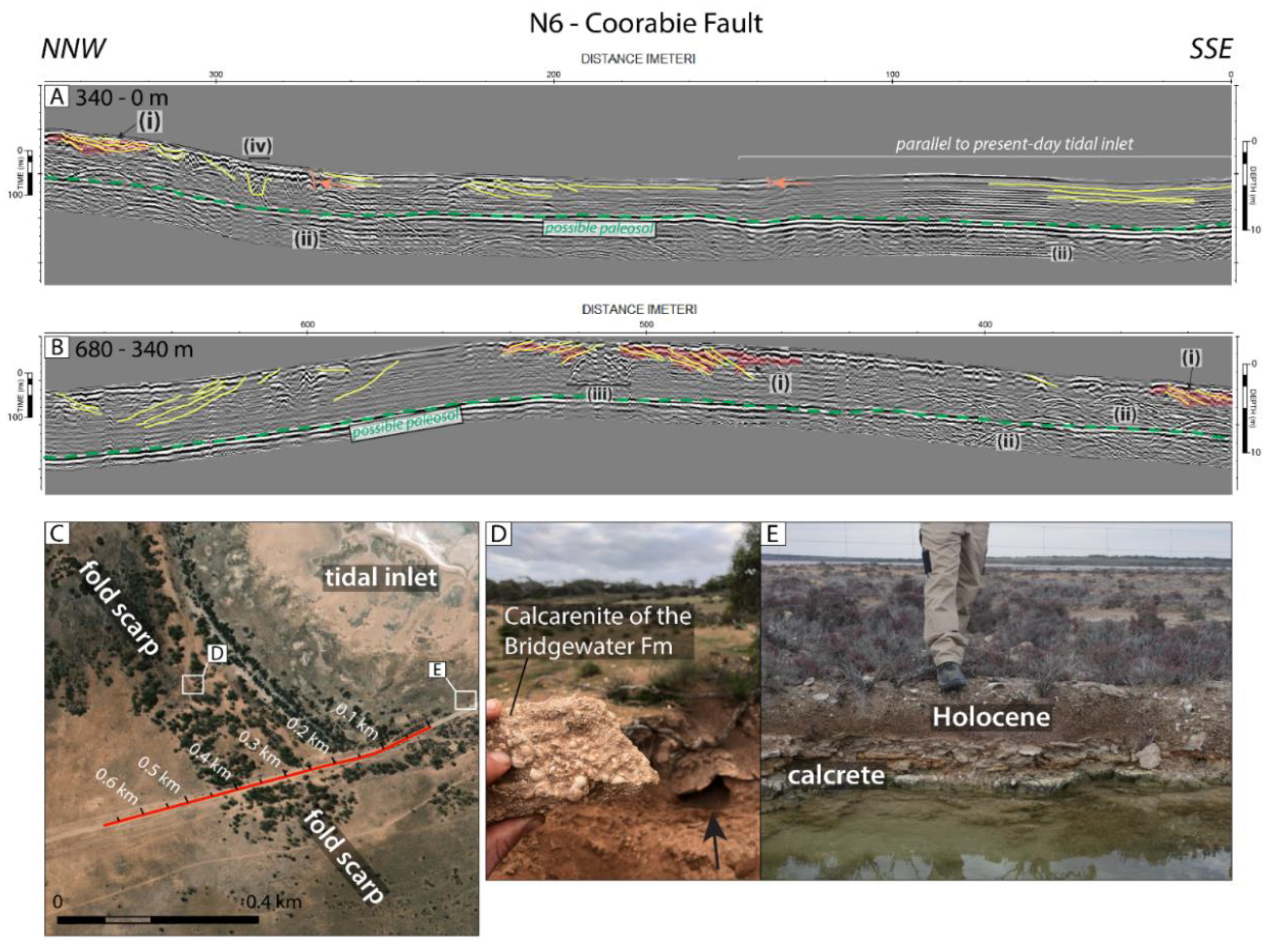
3.2.5. Line N6—Coorabie Fold—Tidal Inlet

Transect N6 was conducted across the scarp of f64 where it bounds the present-day tidal inlet near Fowlers Bay (Figure 4C and Figure 9C). The local surface geology is again characterized by the Bridgewater Formation.

Similar to N4 and N5 a paleo-surface is imaged by a strong and continuous, mostly surface-parallel reflector package at ~5 m depth extending throughout the entire transect (Figure 9A,B, yellow, dashed line). However, its depth increases to ~7.5 m towards the end of the transect (Figure 9B). The calcretized surface of the Bridgewater deposits (Figure 9D) is again imaged by a strong, discontinuous reflector package at ~1–2.5 m depth, becoming more distinct with the transition from the footwall to the scarp at ~270 m (orange arrows): the surface reflectors appear stronger and thicker, however, more disrupted. Simultaneously, the depth of the signal response increases locally to ~4 m underneath the crest of the scarp (Figure 9B). Increased penetration depth usually coincides with locations where distinct reflectors could be identified (yellow solid lines) imaging the sedimentary strata of the Bridgewater deposits. The transect section between 0–~150 m runs parallel to the present-day tidal inlet (Figure 9C). The equivalent GPR data is characterized by horizontally layered, mostly weak reflectors imaging the periodic sedimentation within the tidal inlet. These are obscured by hyperbolic airwave reflections from vegetation and multiples possibly caused by higher clay contents in the sediment. The relatively weak reflectors continue beyond 150 m in the GPR data to ~260 m, proximate to the base of the scarp, interrupted by several inclined reflectors between ~200–230 m. This zone (~150–260 m) may experience flooding only during high tides. Broad wavelength folding is evidenced by continuous paleo-marker at depth without discrete breaks. Hyperbolic diffractions at (iii) and (iv) are likely to image anthropogenic structures, i.e., infilled trenches.

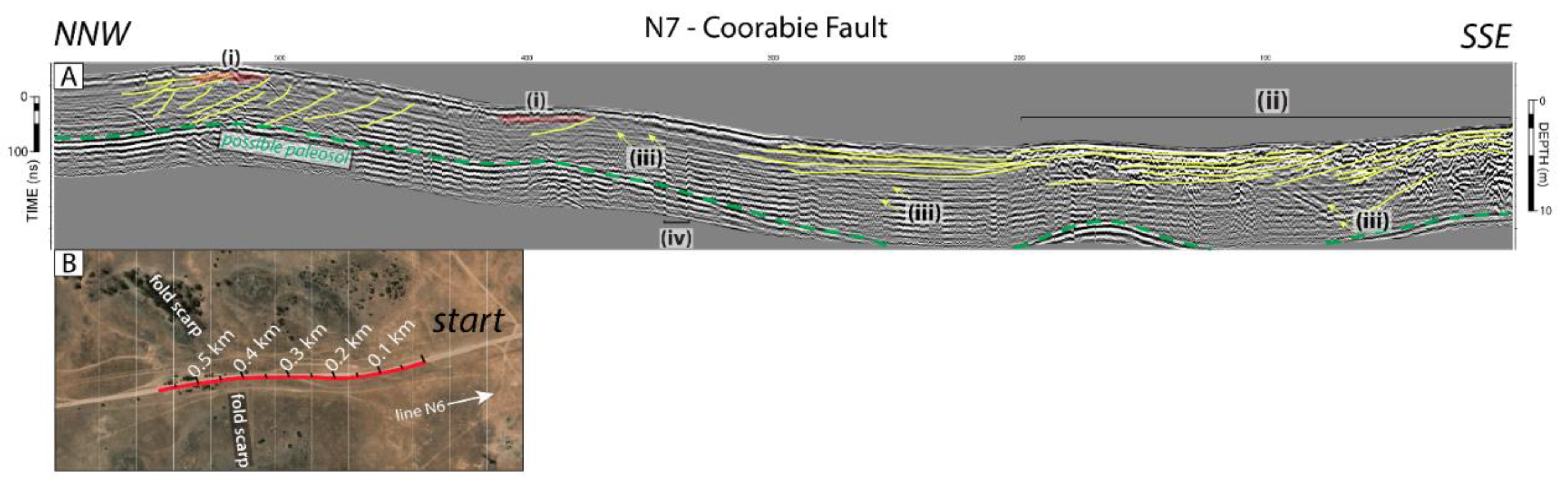
3.2.6. Line N7—Coorabie Fold—Splay

Transect N7 was conducted along the same road as N6, crossing a splay of f64, f673 (Figure 4C), that displaces an older part of the tidal inlet. Like in N4, N5 and N6, a paleo-surface is imaged at depth, however, depth variations from ~5 m to >8 m appear discontinuous between ~70–120 m and ~200–260 m (Figure 10). Overall depth decreases underneath the hanging wall, so that the unit above the strong reflectors overlies the latter unconformably between 0 and ~390 m. Together with surface-parallel reflectors at the base of the scarp this may indicate syn-deformational erosion and corresponding colluvial deposition.

The hanging wall and scarp slope are characterized by mostly parallel layered, weak reflectors, obscured by multiples and few hyperbolic diffractions, with a single, strong, disturbed reflector package at the surface imaging the calcretized surface, whereas an increase in penetration depth and accompanied increase in reflector identification (yellow lines) is spatially limited to the extended footwall (Figure 10A, zone (ii)). Although in this case not related to the hanging wall of f673, similar to lines N4, N5 and N6 maximum penetration depths (~5 m) appear to coincide with elevated topography, i.e., the fold scarp in lines N4, N5 and N6, and two smaller ridges on the footwall in this transect in zone a. Few inclined, curvilinear reflectors were identified underneath the hanging wall imaging crossbedding within the Bridgewater Formation, but are entirely missing underneath the base of the scarp (~200–~340 m) which is most likely due to strong multiples obscuring the GPR signal.

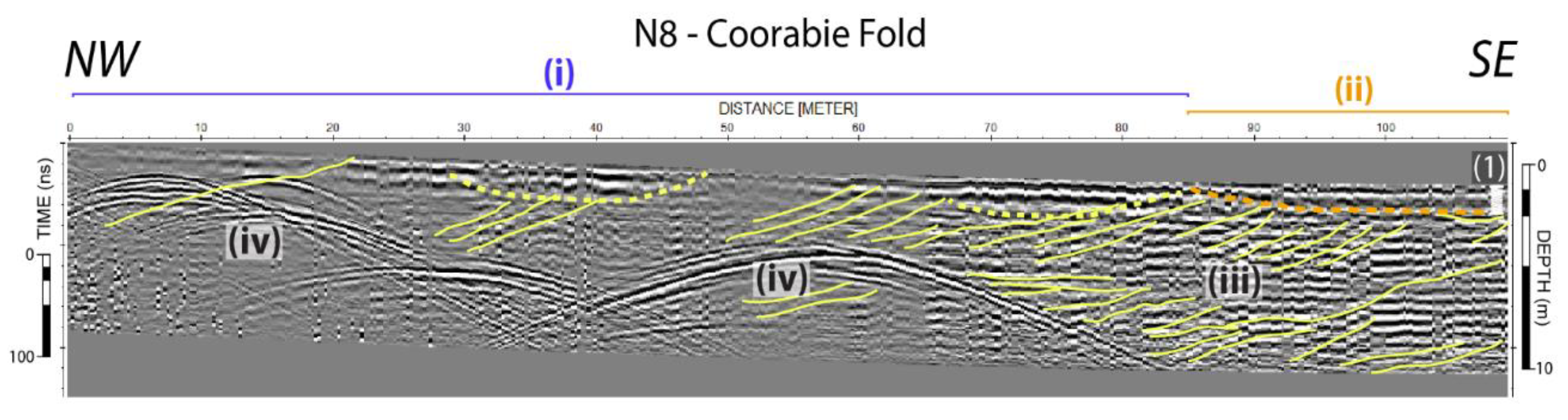
3.2.7. Line N8—Coorabie Fold—Ponding Feature

N8 was conducted at the northern tip of f64 where a large ~100 km² recent ponding feature is located on the footwall at the base of the scarp (Figure 2D). The transect section between 0~85 m correlates with the slope of the fold scarp (zone (i)) and the remaining section correlates with the ponding feature (zone (ii)) (Figure 11). The GPR data along the fold scarp is impacted by hyperbolic diffractions originating from wombat burrows and airwave reflections from larger vegetation, which are not present within the ponding feature, therefore revealing a larger number of reflectors at the base of the scarp (yellow lines) which are likely to image sedimentary strata. Reflectors are overall weak and obscured by multiples, particularly on the footwall, except from a stronger, disrupted surface reflector package of the upper ~2–2.5 m imaging the calcretized surface. The interpreted thickness of the sediment package in the ponding feature (marked by orange, dashed line) correlates with thicknesses identified through augering. Two weak reflectors were identified on the slope of the scarp (dashed, yellow line) exhibiting a bowl-shape, similar to the reflector which marks the base of the present-day ponding feature on the footwall.

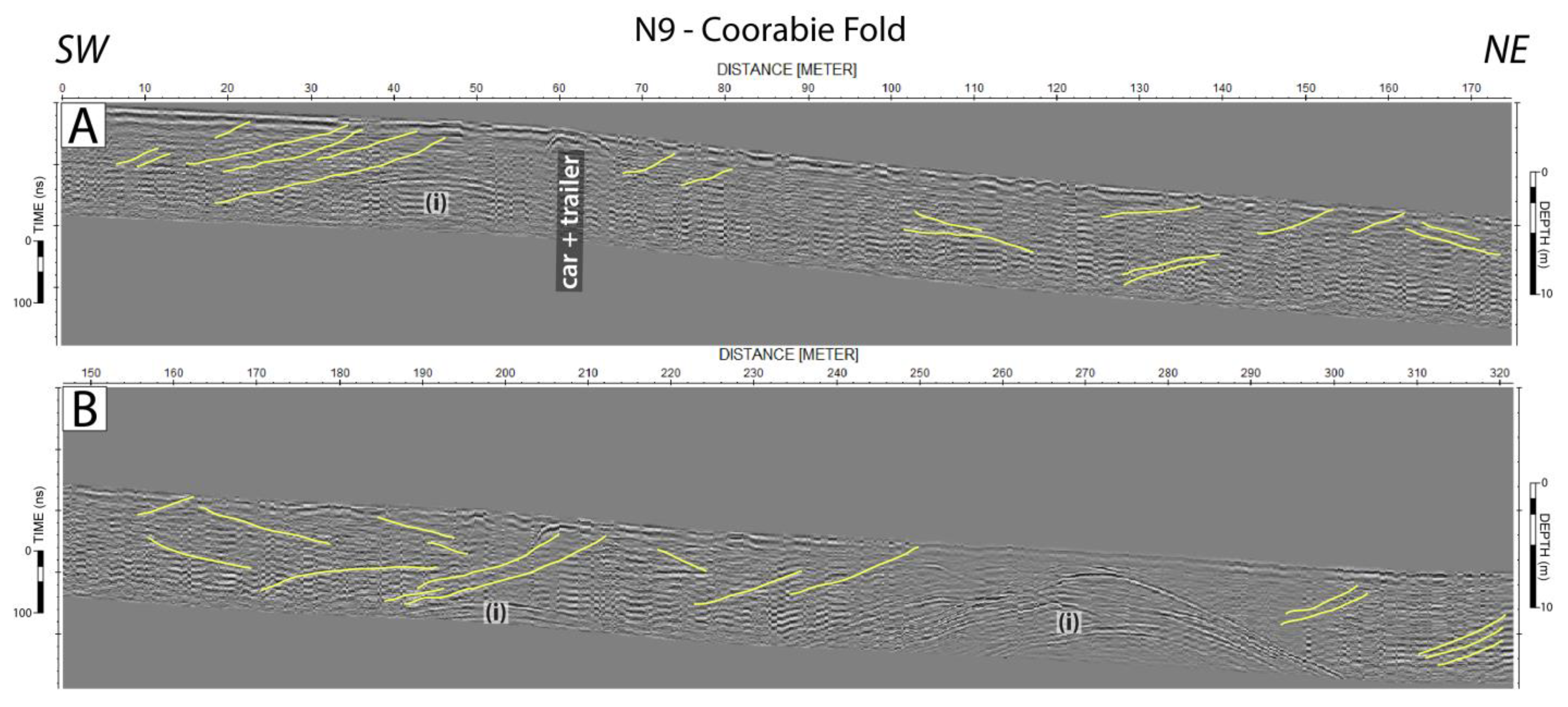
3.2.8. Line N9—Coorabie Fold

This transect is located along the central section of f64, approximately 40 km north of the coast (Figure 2E). The overall signal response along the entire GPR transect is weak, obscured by additional multiples, except from an ~2–2.5 m thick stronger, however, disrupted reflector package at the surface which likely images the local calcrete capping (Figure 12). A few wide hyperbolic diffractions represent airwave reflections from trees and shrubs. Reflectors (yellow solid lines) are interpreted to image sedimentary strata.

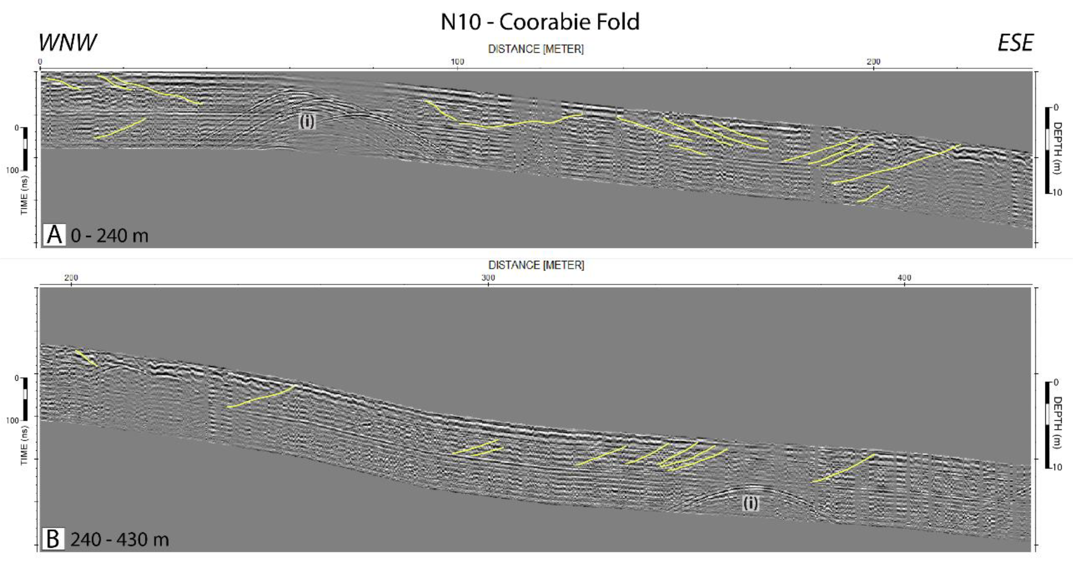
3.2.9. Line N10—Coorabie Fold

GPR transect N10 exhibits similar characteristics as N9: the overall signal response is weak and locally obscured by multiples and airwave reflections from trees (Figure 13). Interpreted reflectors, marked in yellow, are most likely imaging cross-bedded sedimentary strata.

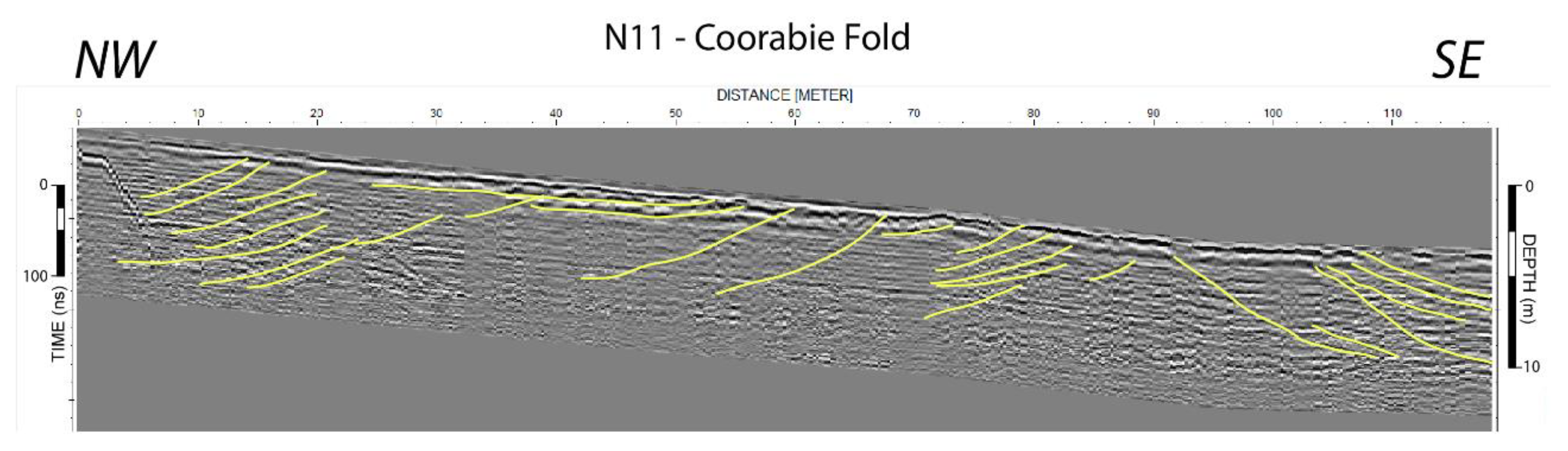
3.2.10. Line N11—Coorabie Fold

The GPR signal response of transect N11 is, again, similar to N9 and N10, with weak reflectors at depth and a ~2 m thick strong surface reflector package imaging calcrete capping (Figure 14). Along the slope of the scarp between 0–~90 m all interpreted reflectors dip downslope, while reflectors at the base of the scarp dip the opposite direction. The change in dip direction coincides with a flattening of topography, possibly implying channelization and/or onlapping sedimentation.

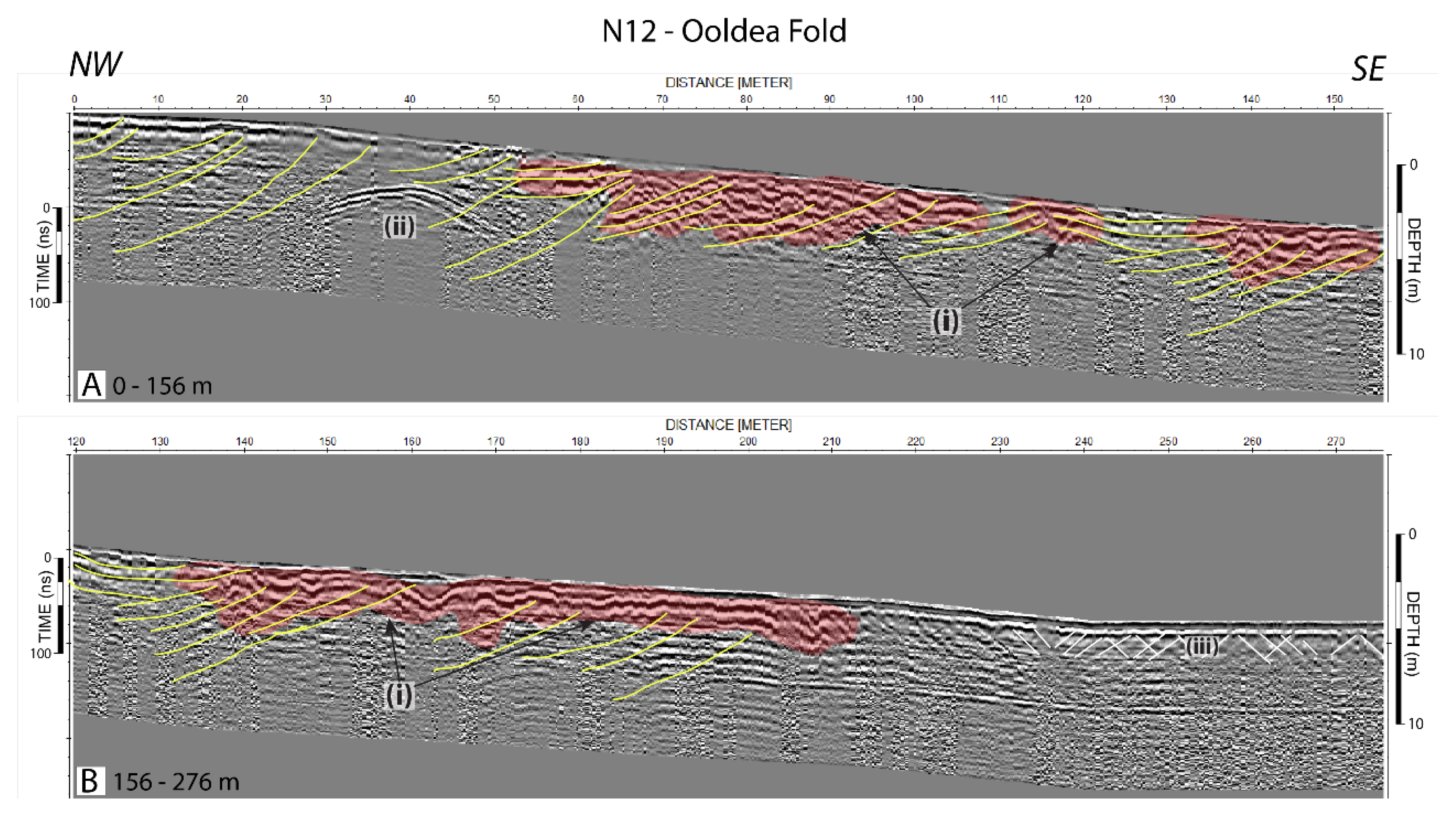
3.2.11. Line N12—Ooldea Fold

Transect N12 was conducted across fold scarp f56 approximately 2.5 km south of its northern tip and the proximate Quaternary dunefields draping the Eocene/Miocene shorelines which surround the Nullarbor Plain (Figure 2F).

Between ~45–210 m the GPR signal consists of strong, disrupted reflector packages with depth up to ~4 m (faint red zones), likely imaging cemented/calcretized zones, whereas the remaining transect sections exhibit mostly weak reflectors with numerous faint hyperbolic diffractions and a thin, ~1 m thick stronger reflector package at the surface (Figure 15). The latter is again interpreted to image local calcrete development. Increased penetration depth along the scarp slope facilitates the identification of reflectors (yellow linework) which we interpret to image sedimentary strata. Variations in dip directions imply crossbedding and perhaps channelization of sediments during deposition. Between ~210 m and the end of the transect a relatively homogenous, perhaps nodular surface calcrete is imaged by a strong reflector package, with numerous, regularly distanced weak hyperbolic diffractions (white solid lines). Underneath, the signal response is overall weaker than along the rest of the transect, possibly due to more clay-rich sedimentation at the base of the scarp.

Although the lithology imaged in the Nullarbor and Roe Plain transects is significantly different from the Willunga site and no references based on, e.g., trenches or transect-adjacent outcrops are available general interpretations can be transferred from the Willunga data.

Features in the GPR data are interpreted as follows:

➢

Strong, mostly horizontal, however, disturbed surface reflectors often interrupted by numerous small hyperbolic diffractions image nodular to tabular calcrete whereas the size of identifiable hyperbolas can be used as a proxy for the relative maturity of calcrete development and hence for relative ages of surfaces.

➢

Strong, disrupted, spatially limited reflector packages at depth mostly occurring in elevated terrain (i.e., underneath hanging walls) represent zones of increased subsurface material alterations (e.g., chemical weathering/mineral precipitation) possibly facilitated by coseismic fracturing and cracking.

➢

Weak, inclined, curvilinear reflectors throughout the main body of the GPR data are interpreted to image structures of the underlying rocks (e.g., limestones and calcarenites of shoreline barriers) such as bedding planes.

➢

Strong, inclined, curvilinear reflectors within the spatially limited reflector packages at depth are interpreted to image structures of the underlying rocks (e.g., limestones and calcarenites of shoreline barriers) such as bedding planes, accentuated through the occurring material alterations in these zones.

➢

Narrow hyperbolic diffractions underlain with a very strong reflector package and a velocity of ~0.12 m/ns, the average propagation velocity of limestone, are interpreted to indicate cavities or fractures in limestone.

➢

Hyperbolic diffractions with a velocity of 0.3 m/ns represent airwave reflections mostly from trees.

4. Discussion

The Willunga Fault is considered to represent an ‘end-member’ within the suite of fault-propagation folds studied here, where possible deformation processes, i.e., fault propagation has breached the surface (Figure 16C). The Nullarbor folds represent stages between an initial surface deformation and a surface breach (Figure 16A,B) where the shallowest rupture tips remain beneath the surface at depths exceeding the GPR imaging depth.

Fracturing, cracking, and flexure, particularly within the hanging wall, is expected to occur and increase with progressing deformation and consequently displacement, while scarp height may be regarded as a proxy for the amount of accumulated displacement. For instance, the Ostler Fault Zone on the South Island of New Zealand, although clearly characterised as surface rupturing thrust fault system, involves hanging wall-folding where fault segments overlap [65] These step-over zones have accumulated less vertical displacement than the adjacent fault segments and instead distributed deformation across a set of splays and therefor a wider deformation zone [65].

Several field campaigns that included field mapping and trenching reveal that the Willunga Fault consists of an imbricate fault system that involves at least three reverse faults on the footwall and a number of flexural structures on the hanging wall (e.g., Figure 3).

The GPR signal images disturbances and thickness changes, particularly within the Quaternary sediments, that are indicative of discrete faulting. Where no faulting is associated with disturbed reflectors, hyperbolic diffractions and reflector disruptions are likely to image colluvial sedimentation, particularly when identified downslope of faults (e.g., feature (iii) in Figure 16C).

For the Nullarbor and Roe Plain GPR transects three main observations are made:

➢

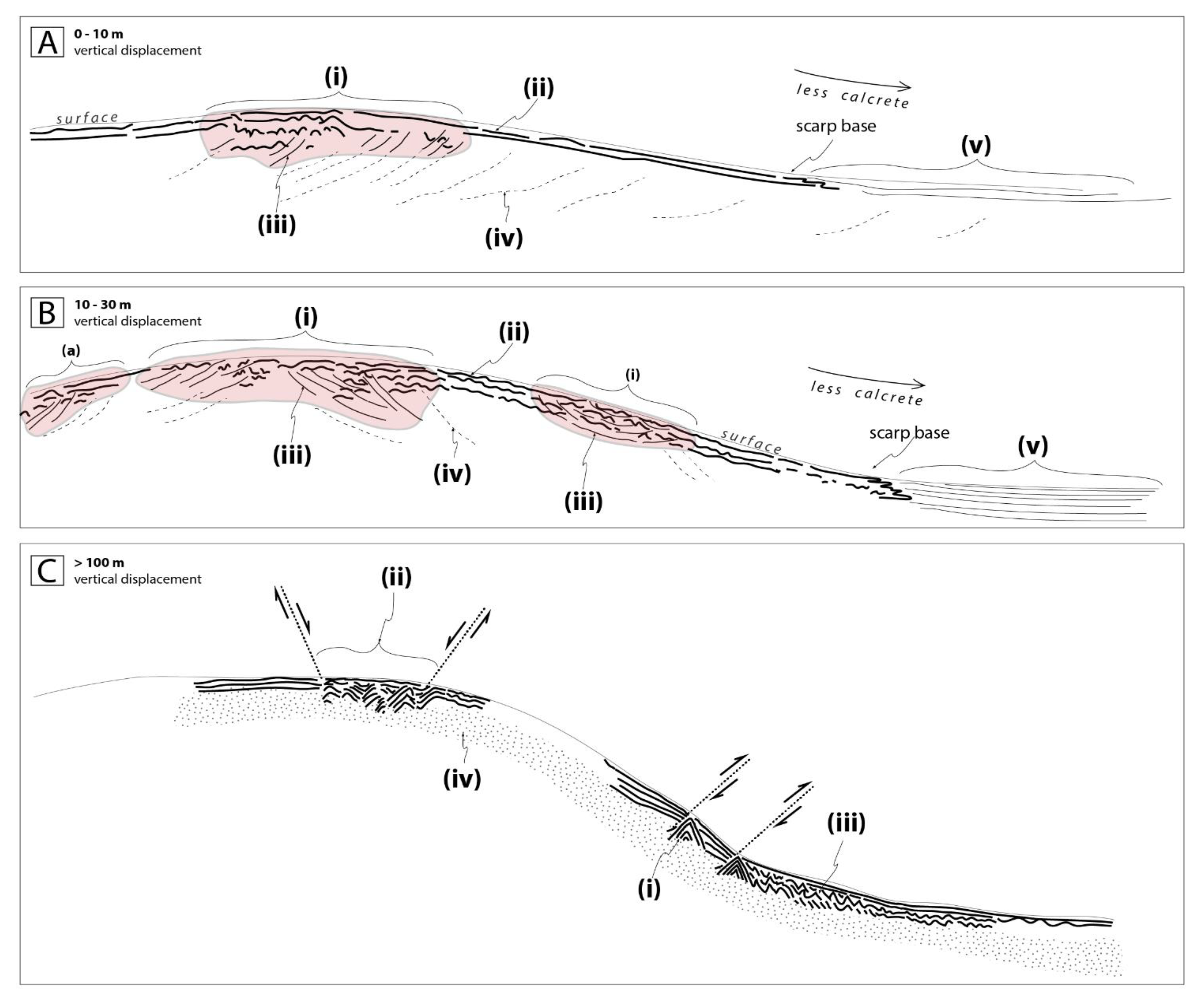
weak reflectors associated with unaltered, calcareous and/or clay-rich material (features (iv) in Figure 16A,B),

➢

strong, max.~2 m thick, variably disturbed (indicated by hyperbolic diffractions), or discontinuous reflector packages imaging calcretization at the present-day surface or of paleosurfaces (features (ii) in Figure 16A,B). Thickness and disturbances, i.e., size and amount of hyperbolic diffractions may be indicative of calcrete maturity, and hence, relative surface ages,

➢

strong, thicker (up to ~4 m) reflector packages, disrupted by hyperbolas, mostly identified in elevated terrain, i.e., hanging walls and scarp slopes (features (i) in Figure 16A,B).

These reflectors are interpreted to image deeper extending calcretization due to possibly favorable conditions and increased accommodation space for calcrete formation in elevated terrain compared to lower lying terrain (Figure 16A,B):

A Pliocene to Pleistocene age for calcrete formation on the Nullarbor Plain has been suggested by [51], possibly indicating that most of the calcrete formed with the transition from the Pliocene wet phase to the present-day arid climate. Calcrete can either form through evaporation in the soil profile, along the capillary fringe or even below the groundwater table (e.g., [72]). During and at the initial termination of the Pliocene wet phase the groundwater table may have been much shallower on the Nullarbor Plain than at present leaving a ‘narrow’ zone for calcrete formation and a maximum formation depth at around the groundwater table (Figure 17A). Overall progressing aridification after the Pliocene would have increased ground water table depths creating more accommodation space for calcrete to form (Figure 17B). The same would take effect where topographic variations, i.e., elevation changes, occur, represented by, e.g., foldscarps or dunes (Figure 17C). Variations in the combination of these three simplified scenarios would obviously depend on regional and local variations in the temporal order of these scenarios, i.e., if folding occurred during the Pliocene wet phase calcrete formation underneath the hanging wall and scarp slope would be expected to be more extensive compared to a scarp that formed during the progressing aridification.

Calcrete formation and other alterations caused by, e.g., chemical (e.g., karstification) and/or mechanical weathering may have been further promoted in response to deformational processes (e.g., cracking, fracturing) providing deeper extending pathways for fluids. These may additionally exploit other existing ‘weak zones’, such as bedding planes so that material alterations and cementation along these weak zones would produce stronger contrast changes and, hence, stronger reflectors. This highlights otherwise weakly imaged sedimentary structures (features (iv) in Figure 16A,B) as stronger reflectors (features (iii) in Figure 16A,B) where they coincide with zones of stronger reflector packages (features (i) in Figure 16A,B; also Figure 5A, Figure 9B and Figure 15). Possible trends in the relationship between the GPR signal response and the scarp height are observed for certain transects when grouped by local near surface geology:

N1, N2, N3 and N12, with max. vertical displacements of ~24 m, ~8 m, ~4 m and ~12 m, respectively, are located within Nullarbor Limestone. The number of strong reflector packages clearly is highest in N1, followed by N12, while the only strong signal response in N2 is produced by the calcrete capping. However, the near surface materials at N2 are characterised by undefined residual sediments and calcrete [73] of unknown thickness and the location of the transect has been additionally influenced by fluvial sedimentation so that the GPR signal may be attenuated by clay-rich sediments. Similarly, only the calcretized calcarenite cover of the Roe Plain produced a strong signal response along N3 and only few reflectors (yellow lines), presumably imaging sedimentary strata in the underlying Abrakurrie Limestones were identified, although a similar GPR structure may have been expected as along N1 because both transects cross the same fold scarp (f290). However, the Nullarbor limestone surface, and with it the vertical displacement along the southern section of f290 were removed with formation of the present-day Roe Plain (e.g., [17]). Hence, the original, post-seismic structure within the Nullarbor Limestones was removed, leaving only the Abrakurrie Limestones which may not have experienced any deformation-related alterations at their original depth. Renewed deformation along f290 post-Roe Plain formation, evidenced by the present-day ~5 m high scarp across the Plain, may then not have been sufficient or too recent to cause alterations in the near-surface materials. Additionally, N3 is heavily impacted by diffractions and reflections obscuring most of the transect at depth.

The four transects within the Bridgewater Formation, N4–N7, with max. vertical displacements of ~5, ~4, ~24, and ~7.5 m, respectively, appear to indicate an increase in localized stronger reflector packages on the hanging wall with increasing vertical displacement (reddish zones). Some reflector packages in N4 and N5 (features (iv)) may also represent localised paleo horizons as their signal structure is similar to the reflectors imaging the present-day calcrete surface.

Transect N7, which was conducted across the same fold scarp as N4 and N5, i.e., f673, appears to be an exception, in that the scarp is slightly higher than at N4 and N5, but the overall signal response below the calcrete surface is weak. The most extensive, strong, and disturbed reflector package along the transect is located where the transect rises to a gentle ridge between lines N6 and N7 (Figure 4 and Figure 10, zone (i)). Whether this ridge may represent an unidentified scarp, or an undeformed dune ridge is unclear, however, the extent of strong reflector packages implies that this section has been subject to calcrete capping for much longer than the fold scarp.

Overall, variations in signal response, whether caused by alterations through induration or deformation induced weathering, appear to be focused on the hanging walls and scarp slopes.

The transects N8–N11, all conducted across fold scarp f64 and located within Pleistocene, calcareous gravels, clays, silts and sand, do not exhibit any strong reflector packages at depth, except from a surface reflector package of the uppermost ~2 m imaging calcrete capping (Figure 11, Figure 12, Figure 13 and Figure 14). The main body of the GPR data is characterised by weak reflectors which are likely imaging (cross-bedded and/or channelised) sedimentary structure. No evidence for faulting or folding is observed from the GPR data which we interpret to be due to a rather unconsolidated nature of the local sediments, compared to the limestones or more intensively indurated deposits of the, e.g., Bridgewater Formation.

Changes in signal amplitude and velocities identified from hyperbolic diffractions are indicative of different subsurface materials, i.e., lithologies. Their occurrence will not only influence the structural manifestation of coseismic deformation at the surface and in the subsurface but may be used to decipher the temporal relationships between deformation and material deposition.

At the Willunga Fault site only a few meters of mostly unconsolidated sediments are deposited on top of the Precambrian basement rocks. In contrast, ~700 m of Cretaceous and Cenozoic sediment lies above the basement in the Eucla Basin and mostly brittle limestones and partially calcretized calcarenites of the coastal Bridgewater Formation and calcareous clays, silts and sand of the easternmost Nullarbor Plain are present.

This will impact the GPR signal response (e.g., are contrast changes strong enough to produce identifiable reflectors?) but also the signal patterns (i.e., the amplitude) and their distribution in accordance to the geological deformation response. I.e., interpreted reflectors in line N1 exhibit sedimentary onlap during fold growth implying deformation along f91 during limestone deposition. Along line N7 sediment thickness above the paleosurface increases towards the footwall and no discrete break in the subsurface reflector or surface strata is observed. This implies the formation of accommodation space during broad wavelength folding for sediments to be deposited on the footwall obscuring the base of the scarp. Displacement represented by the present-day scarp height would then not represent the total displacement originally produced because the vertical distance between the crest of the scarp and the footwall surface has been reduced.

Other transects, e.g., N4 and N5, possibly reflect progressive uplift through downslope migrating channel beds. Lastly, variations in size and amount of hyperbolic diffractions within interpreted calcrete capping can provide information about relative ages of surfaces.

The GPR data collected in this study provides information about the structural subsurface deformation response across fault and fold scarps in varying geological environments and highlights the influences of geological and structural heterogeneity on surface deformation styles. It is, however, obvious that future work requires improvements in the acquisition process to improve, e.g., the data resolution and confidence in interpreted features. Additional work should involve (i) the detailed mapping of exemplary exposures within the targeted geological units and comparison of observed features with matching features in the GPR signal (e.g., [74]), (ii) 3-D or several closely spaced 2-D surveys to improve information about the spatial distribution of identified features (e.g., [64,75]), (iii) the application of different frequencies adjusted according to anticipated penetration depths and associated velocities, and (iv) further improvements during the processing of the GPR data.

5. Conclusions

• GPR transects across the Willunga Fault south of Adelaide provide evidence for imbricate reverse faulting and flexural hanging wall deformation that is consistent with field data. GPR can assist in identifying prospective sites for paleoseismological investigations in low slip-rate, distributed fault zones.
• No discrete fault traces were identified along the Nullarbor and Roe Plain GPR transects.
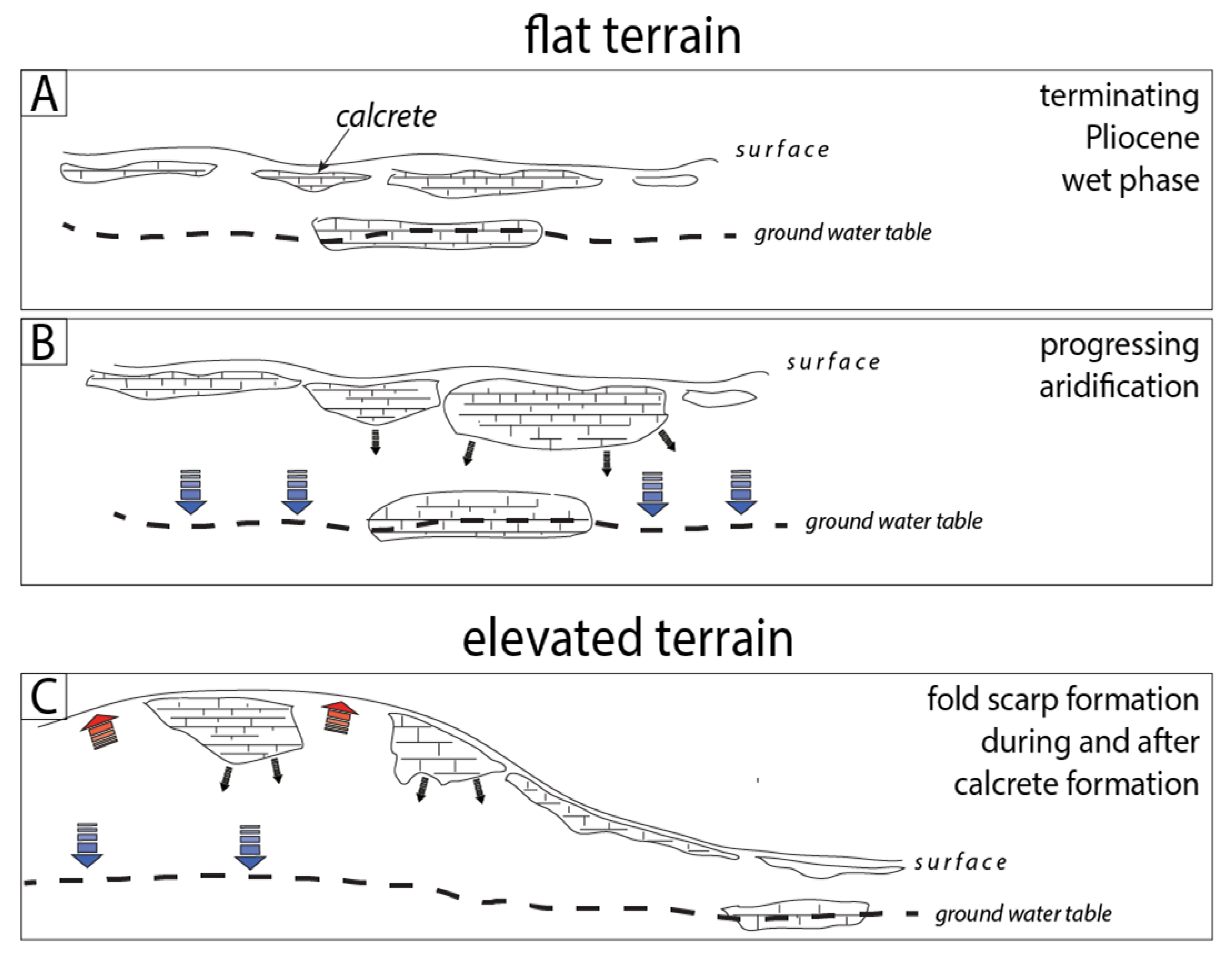
• Despite the general uniformity of the lithology across the Nullarbor and Roe Plain fold scarps, i.e., the lack of strong contrasts between, e.g., unconsolidated vs. consolidated materials, stronger reflector packages appear to be concentrated within the hanging wall and scarp slope sections. These stronger reflector packages are interpreted to represent different stages of calcrete formation and/or material alterations through, e.g., chemical weathering possibly indicative of the temporal relationship between surface deformation and calcrete formation.
• Variations in scarp morphologies, i.e., shallow vs. steep scarp gradients across identified neotectonic folds, monoclines, or discrete faults, are characteristic of different stages of scarp formation and slip transfer to the surface.
• The structural evolution of the scarp may hereby involve progressive fault-propagation folding (e.g., Nullarbor folds) and eventual surface rupture (e.g., Willunga Fault). However, surface ruptures may form without preceding fault-propagation folding (e.g., [30]). This is highly dependent on the local near-surface materials.
• Identification of these different stages, associated extent of the damage zone and how cumulative displacement is distributed within the damage zone may inform the future spatial evolution of the damage zone and, by extension, may provide important input for seismic hazard analysis.
• Assessment of scarp ‘maturity’, associated extent of the damage zone and how cumulative displacement is distributed within the damage zone may inform the future spatial evolution of the damage zone.

References

- Brozzetti, F.; Boncio, P.; Cirillo, D.; Ferrarini, F.; De Nardis, R.; Testa, A.; Liberi, F.; Lavecchia, G. High-Resolution Field Mapping and Analysis of the August–October 2016 Coseismic Surface Faulting (Central Italy Earthquakes): Slip Distribution, Parameterization, and Comparison with Global Earthquakes. Tectonics 2019, 38, 417–439. [Google Scholar] [CrossRef] [Green Version]
- Fletcher, J.M.; Teran, O.J.; Rockwell, T.K.; Oskin, M.E.; Hudnut, K.W.; Mueller, K.J.; Spelz, R.M.; Akciz, S.O.; Masana, E.; Faneros, G.; et al. Assembly of a large earthquake from a complex fault system: Surface rupture kinematics of the 4 April 2010 El Mayor–Cucapah (Mexico) Mw 7.2 earthquake. Geosphere 2014, 10, 797–827. [Google Scholar] [CrossRef] [Green Version]
- Bello, S.; Scott, C.P.; Ferrarini, F.; Brozzetti, F.; Scott, T.; Cirillo, D.; de Nardis, R.; Arrowsmith, J.R.; Lavecchia, G. High-resolution surface faulting from the 1983 Idaho Lost River Fault Mw 6.9 earthquake and previous events. Sci. Data 2021, 8, 68. [Google Scholar] [CrossRef] [PubMed]
- King, G.C.P.; Stein, R.S.; Rundle, J.B. The Growth of Geological Structures by Repeated Earthquakes 1. Conceptual Framework. J. Geophys. Res. Earth Surf. 1988, 93, 13307–13318. [Google Scholar] [CrossRef]
- Livio, F.A.; Berlusconi, A.; Michetti, A.M.; Sileo, G.; Zerboni, A.; Trombino, L.; Cremaschi, M.; Mueller, K.; Vittori, E.; Carcano, C.; et al. Active fault-related folding in the epicentral area of the December 25, 1222 (Io=IX MCS) Brescia earthquake (Northern Italy): Seismotectonic implications. Tectonophysics 2009, 476, 320–335. [Google Scholar] [CrossRef]
- McKay, L.; Lunn, R.; Shipton, Z.; Pytharouli, S.; Roberts, J. Do intraplate and plate boundary fault systems evolve in a similar way with repeated slip events? Earth Planet. Sci. Lett. 2021, 559, 116757. [Google Scholar] [CrossRef]
- Bergen, K.J.; Shaw, J.H. Displacement profiles and displacement-length scaling relationships of thrust faults constrained by seismic-reflection data. GSA Bull. 2010, 122, 1209–1219. [Google Scholar] [CrossRef]
- Davis, K.; Burbank, D.W.; Fisher, D.; Wallace, S.; Nobes, D. Thrust-fault growth and segment linkage in the active Ostler fault zone, New Zealand. J. Struct. Geol. 2005, 27, 1528–1546. [Google Scholar] [CrossRef]
- Kelson, K.I.; Kang, K.H.; Page, W.D.; Lee, C.T.; Cluff, L.S. Representative Styles of Deformation along the Chelungpu Fault from the 1999 Chi-Chi (Taiwan) Earthquake: Geomorphic Characteristics and Responses of Man-Made Structures. Bull. Seism. Soc. Am. 2001, 91, 930–952. [Google Scholar] [CrossRef]
- Philip, H.; Meghraoui, M. Structural analysis and interpretation of the surface deformations of the El Asnam Earthquake of October 10, 1980. Tectonics 1983, 2, 17–49. [Google Scholar] [CrossRef]
- Ruegg, J.C.; Kasser, M.; Tarantola, A.; Lepine, J.C.; Chouikrat, B. Deformations associated with the El Asnam earthquake of 10 October 1980: Geodetic determination of vertical and horizontal movements. Bull. Seism. Soc. Am. 1982, 72, 2227–2244. [Google Scholar] [CrossRef]
- Bello, S.; Andrenacci, C.; Cirillo, D.; Scott, C.P.; Brozzetti, F.; Arrowsmith, J.R.; Lavecchia, G. High-Detail Fault Segmentation: Deep Insight into the Anatomy of the 1983 Borah Peak Earthquake Rupture Zone (Mw 6.9, Idaho, USA). Lithosphere 2022, 2022, 8100224. [Google Scholar] [CrossRef]
- Ferrario, M.F.; Livio, F. Characterizing the Distributed Faulting During the 30 October 2016, Central Italy Earthquake: A Reference for Fault Displacement Hazard Assessment. Tectonics 2018, 37, 1256–1273. [Google Scholar] [CrossRef]
- Ferrario, M.F.; Livio, F. Distributed faulting following normal earthquakes: Reassessment and updating of scaling relations. Solid Earth 2020, 1, 1–19. [Google Scholar] [CrossRef]
- Oskin, M.E.; Arrowsmith, J.R.; Corona, A.H.; Elliott, A.J.; Fletcher, J.M.; Fielding, E.J.; Gold, P.O.; Garcia, J.J.G.; Hudnut, K.W.; Liu-Zeng, J.; et al. Near-Field Deformation from the El Mayor–Cucapah Earthquake Revealed by Differential LIDAR. Science 2012, 335, 702–705. [Google Scholar] [CrossRef] [PubMed] [Green Version]
- Zinke, R.; Hollingsworth, J.; Dolan, J.F. Surface slip and off-fault deformation patterns in the 2013 MW7.7 Balochistan, Pakistan earthquake: Implications for controls on the distribution of near-surface coseismic slip. Geochem. Geophys. Geosystems 2014, 15, 5034–5050. [Google Scholar] [CrossRef]
- Sellmann, S.; Quigley, M.; Duffy, B.; Yang, H.; Clark, D. Fault geometry and slip rates from the Nullarbor and Roe Plains of south-central Australia: Insights into the spatial and temporal characteristics of intraplate seismicity. Earth Surf. Process. Landforms, 2022; in press. [Google Scholar] [CrossRef]
- Kuang, K. Paleoseismology and Landscape Evolution of the Willunga Fault, Mount Lofty Ranges. Master’s Thesis, University of Melbourne, Melbourne, VIC, Australia, 2018. Unpublished. [Google Scholar]
- Hughes, A.N.; Benesh, N.P.; Shaw, J.H. Factors that control the development of fault-bend versus fault-propagation folds: Insights from mechanical models based on the discrete element method (DEM). J. Struct. Geol. 2014, 68, 121–141. [Google Scholar] [CrossRef]
- Allen, T.I. Seismic hazard estimation in stable continental regions: Does PSHA meet the needs for modern engineering design in Australia? Bull. N. Z. Soc. Earthq. Eng. 2020, 53, 22–36. [Google Scholar] [CrossRef] [Green Version]
- Coppersmith, K.; Youngs, R. Data needs for probabilistic fault displacement hazard analysis. J. Geodyn. 2000, 29, 329–343. [Google Scholar] [CrossRef]
- Moss, R.E.S.; Ross, Z.E. Probabilistic Fault Displacement Hazard Analysis for Reverse Faults. Bull. Seism. Soc. Am. 2011, 101, 1542–1553. [Google Scholar] [CrossRef]
- Youngs, R.R.; Arabasz, W.J.; Anderson, R.E.; Ramelli, A.R.; Ake, J.P.; Slemmons, D.B.; McCalpin, J.P.; Doser, D.I.; Fridrich, C.J.; Swan, F.H., III; et al. A Methodology for Probabilistic Fault Displacement Hazard Analysis (PFDHA). Earthq. Spectra 2003, 19, 191–219. [Google Scholar] [CrossRef]
- Clark, D. Neotectonic Features Database; Geoscience Australia, Commonwealth of Australia: Canberra, Australia, 2012.
- Yang, H.; Sellmann, S.; Quigley, M. Fluid-enhanced neotectonic faulting in the cratonic lithosphere of the Nullarbor Plain in south-central Australia. Geophys. Res. Lett. 2022, 49, e2022GL099155. [Google Scholar] [CrossRef]
- Webb, J.A.; James, J.M. Karst evolution of the Nullarbor Plain, Australia. Geol. Soc. Am. Spec. Pap. 2006, 404, 65. [Google Scholar] [CrossRef]
- Quigley, M.C.; Cupper, M.L.; Sandiford, M. Quaternary faults of south-central Australia: Palaeoseismicity, slip rates and origin. Aust. J. Earth Sci. 2006, 53, 285–301. [Google Scholar] [CrossRef]
- Terzic, Z.R.; Quigley, M.C.; Lopez, F. Detailed Seismic Hazard assessment of Mt Bold area: Comprehensive site-specific investigations on Willunga Fault. In Proceedings of the ANCOLD 2017 Conference Proceedings, Hobart, Tasmania, 26–27 October 2017. [Google Scholar]
- Quigley, M.; Clark, D.; Sandiford, M. Tectonic geomorphology of Australia. Geol. Soc. Lond. Spéc. Publ. 2010, 346, 243–265. [Google Scholar] [CrossRef]
- King, T.R.; Quigley, M.; Clark, D. Surface-Rupturing Historical Earthquakes in Australia and Their Environmental Effects: New Insights from Re-Analyses of Observational Data. Geosciences 2019, 9, 408. [Google Scholar] [CrossRef] [Green Version]
- Amos, C.B.; Burbank, D.W.; Nobes, D.C.; Read, S.A.L. Geomorphic constraints on listric thrust faulting: Implications for active deformation in the Mackenzie Basin, South Island, New Zealand. J. Geophys. Res. Earth Surf. 2007, 112. [Google Scholar] [CrossRef] [Green Version]
- McClymont, A.F.; Green, A.G.; Villamor, P.; Horstmeyer, H.; Grass, C.; Nobes, D.C. Characterization of the shallow structures of active fault zones using 3-D ground-penetrating radar data. J. Geophys. Res. Earth Surf. 2008, 113. [Google Scholar] [CrossRef]
- Clark, D.; McPherson, A.; Cupper, M.; Collins, C.D.N.; Nelson, G. The Cadell Fault, southeastern Australia: A record of temporally clustered morphogenic seismicity in a low-strain intraplate region. Geol. Soc. Lond. Spéc. Publ. 2015, 432, 163–185. [Google Scholar] [CrossRef]
- Dentith, M.; O’Neill, A.; Clark, D. Ground penetrating radar as a means of studying palaeofault scarps in a deeply weathered terrain, southwestern Western Australia. J. Appl. Geophys. 2010, 72, 92–101. [Google Scholar] [CrossRef]
- Drexel, J.F.; Preiss, W.V.; Parker, A.J. (Eds.) The geology of South Australia. In The Precambrian; Geological Survey of South Australia: Adelaide, SA, Australia, 1993; Volume 1, pp. 102–105. 242p. [Google Scholar]
- Drexel, J.F.; Preiss, W.V. (Eds.) The Geology of South Australia. In The Phanerozoic; Geological Survey of South Australia: Adelaide, SA, Australia, 1995; Volume 2, 347p. [Google Scholar]
- Clark, D.; McPherson ACollins, C. Australia’s seismogenic neotectonic record. Geosci. Aust. Rec. 2011, 11, 1–95. [Google Scholar]
- Preiss, W.V. The tectonic history of Adelaide’s scarp-forming faults. Aust. J. Earth Sci. 2019, 66, 305–365. [Google Scholar] [CrossRef]
- Australian Stratigraphic Units Database. Available online: https://asud.ga.gov.au/search-stratigraphic-units/results/8214 (accessed on 18 May 2022).
- Wilson, A. Paleoseismology and Landscape Evolution of the Willunga Fault, Mount Lofty Ranges. Master’s Thesis, University of Melbourne, Melbourne, VIC, Australia, 2018. Unpublished. [Google Scholar]
- Clark, D.; Griffin, J.; La Greca, J.; Quigley, M.; Sellmann, S.; Ninis, D.; Kuang, K.; Wilson, A. Large earthquake recurrence on the Willunga Fault, South Australia [Abstract]. In Proceedings of the Australian Earthquake Engineering Society 2022 National Conference, Mount Macedon, VIC, Australia, 24–25 November 2022. [Google Scholar]
- Dutch, R.A.; Pawley, M.J.; Wise, T.W. What Lies Beneath the Western Gawler Craton? 13GA-EG1E Seismic and Magnetotelluric Workshop 2015, Report Book 2015/00029; Department of State Development: Adelaide, SA, Australia, 2015.
- Nakamura, A.; Milligan, P.R. Total Magnetic Intensity (TMI) Grid of Australia 2015—Sixth Edition, Geoscience Australia, Canberra. Available online: https://ecat.ga.gov.au/geonetwork/srv/eng/catalog.search#/metadata/89595 (accessed on 14 May 2019).
- Nakamura, A. Isostatic Residual Gravity Anomaly Colour Composite Image of Onshore Australia 2016, Geoscience Australia, Canberra. Available online: https://ecat.ga.gov.au/geonetwork/srv/eng/catalog.search#/metadata/101106 (accessed on 16 May 2019).
- Spaggiari, C.V.; Tyler, I.M. (Eds.) Albany–Fraser Orogen Seismic and Magnetotelluric (MT) Workshop 2014: Extended Abstracts: Geological Survey of Western Australia, Record 2014/6; Geological Survey of Western Australia: Adelaide, SA, Australia, 2014; 182p.
- Yang, H.; Quigley, M.; King, T. Surface slip distributions and geometric complexity of intraplate reverse-faulting earthquakes. GSA Bull. 2021, 133, 1909–1929. [Google Scholar] [CrossRef]
- Hocking, R.M. Eucla basin, Western Australia Geological Survey Memoir. Earth Surf. Process. Landf. 1990, 3, 548–561. [Google Scholar]
- Hill, A.J. Bight Basin. In The Geology of South Australia. Vol. 2, The Phanerozoic; Drexel, J.F., Preiss, W.V., Eds.; Geological Survey of South Australia: Adelaide, SA, Australia, 1995; pp. 133–137. [Google Scholar]
- Feary, D.A.; Hine, A.C.; Malone, M.J. Proceedings of the Ocean Drilling Program, 182 Initial Reports; Ocean Drilling Program: College Station, TX, USA, 2000. [Google Scholar] [CrossRef]
- Feary, D.A.; James, N.P. Seismic stratigraphy and geological evolution of the Cenozoic, cool- water Eucla Platform, Great Australian Bight. AAPG Bull. Am. Assoc. Petr. Geol. 2000, 85, 792–816. [Google Scholar]
- Lowry, D.C. Geology of the Western Australian Part of the Eucla Basin; Geological Survey of Western Australia: Perth, WA, Australia, 1970.
- Benbow, M. Tertiary coastal dunes of the Eucla Basin, Australia. Geomorphology 1990, 3, 9–29. [Google Scholar] [CrossRef]
- O’Connell, L.G.; James, N.P.; Bone, Y. The Miocene Nullarbor Limestone, southern Australia; deposition on a vast subtropical epeiric platform. Sediment. Geol. 2012, 253–254, 1–16. [Google Scholar] [CrossRef]
- German Aerospace Centre. TanDEM-X Ground Segment, DEM Products Specification Document TD-GS-PS-0021. 2016. Available online: https://tandemx-science.dlr.de/ (accessed on 19 April 2020).
- NASA Shuttle Radar Topography Mission (SRTM). Shuttle Radar Topography Mission (SRTM) Global, Distributed by OpenTopography. 2013. Available online: https://portal.opentopography.org/datasetMetadata?otCollectionID=OT.042013.4326.1 (accessed on 15 May 2020).
- Cirillo, D.; Cerritelli, F.; Agostini, S.; Bello, S.; Lavecchia, G.; Brozzetti, F. Integrating Post-Processing Kinematic (PPK)–Structure-from-Motion (SfM) with Unmanned Aerial Vehicle (UAV) Photogrammetry and Digital Field Mapping for Structural Geological Analysis. ISPRS Int. J. Geo-Inform. 2022, 11, 437. [Google Scholar] [CrossRef]
- Crosby, C.J.; Arrowsmith, J.R.; Nandigam, V. Zero to a trillion: Advancing Earth surface process studies with open access to high-resolution topography. Dev. Earth Surf. Process. 2020, 23, 317–338. [Google Scholar] [CrossRef]
- Johnson, K.; Nissen, E.; Saripalli, S.; Arrowsmith, J.R.; Mcgarey, P.; Scharer, K.; Williams, P.; Blisniuk, K. Rapid mapping of ultrafine fault zone topography with structure from motion. Geosphere 2014, 10, 969–986. [Google Scholar] [CrossRef]
- Westoby, M.; Brasington, J.; Glasser, N.F.; Hambrey, M.J.; Reynolds, J.M. ‘Structure-from-Motion’ photogrammetry: A low-cost, effective tool for geoscience applications. Geomorphology 2012, 179, 300–314. [Google Scholar] [CrossRef]
- Beres, M.; Haeni, F.P. Application of Ground-Penetrating-Radar Methods in Hydrogeologie Studies. Ground Water 1991, 29, 375–386. [Google Scholar] [CrossRef]
- Daniels, D.J. Ground Penetrating Radar, 2nd ed.; IEE Radar, Sonar and Navigation Series 15; Institution of Electrical Engineers: London, UK, 2004; ISBN 9780863413605. [Google Scholar] [CrossRef] [Green Version]
- Figueiredo, P.; Hill, J.; Merschat, A.; Scheip, C.; Stewart, K.; Owen, L.; Wooten, R.; Carter, M.; Szymanski, E.; Horton, S.; et al. The Mw 5.1, 9 August 2020, Sparta Earthquake, North Carolina: The First Documented Seismic Surface Rupture in the Eastern United States. GSA Today 2022, 32, 4–11. [Google Scholar] [CrossRef]
- Hornblow, S.; Quigley, M.; Nicol, A.; Van Dissen, R.; Wang, N. Paleoseismology of the 2010 Mw 7.1 Darfield (Canterbury) earthquake source, Greendale Fault, New Zealand. Tectonophysics 2014, 637, 178–190. [Google Scholar] [CrossRef]
- McClymont, A.F.; Green, A.G.; Streich, R.; Horstmeyer, H.; Tronicke, J.; Nobes, D.C.; Pettinga, J.; Campbell, J.; Langridge, R. Visualization of active faults using geometric attributes of 3D GPR data: An example from the Alpine Fault Zone, New Zealand. Geophys. 2008, 73, B11–B23. [Google Scholar] [CrossRef] [Green Version]
- Wallace, S.C.; Nobes, D.C.; Davis, K.J.; Burbank, D.W.; White, A. Three-dimensional GPR imaging of the Benmore anticline and step-over of the Ostler Fault, South Island, New Zealand. Geophys. J. Int. 2010, 180, 465–474. [Google Scholar] [CrossRef] [Green Version]
- James, N.P.; Bone, Y.; Carter, R.M.; Murray-Wallace, C.V. Origin of the Late Neogene Roe Plains and their calcarenite veneer: Implications for sedimentology and tectonics in the Great Australian Bight. Aust. J. Earth Sci. 2006, 53, 407–419. [Google Scholar] [CrossRef]
- Geological Survey of South Australia, Department of State Development, SA Geological Atlas Series Sheet SH5212, OOLDEA, 1:250,000, Adelaide, 2012. Available online: https://products.sarig.sa.gov.au/Products/Index/230 (accessed on 16 August 2018).
- Australian Stratigraphic Units Database. Available online: https://asud.ga.gov.au/search-stratigraphic-units/results/2543 (accessed on 3 September 2022).
- Geological Survey of South Australia, Department of State Development, SA Geological Atlas Series Sheet SH5313, FOWLER, 1:250,000, Adelaide, 2015. Available online: https://products.sarig.sa.gov.au/Products/Index/230 (accessed on 16 August 2018).
- Lipar, M.; Ferk, M.; Šmuc, A.; Barham, M. Enigmatic annular landform on a Miocene planar karst surface, Nullarbor Plain, Australia. Earth Surf. Process. Landforms, 2022; in press. [Google Scholar] [CrossRef]
- Belperio, A.P. Fowlers Bay Rotary Drilling Report and Revision of the Quaternary Geology around Fowlers Bay. Report Book No. 1988/93; Department of Mines and Energy: Adelaide, SA, Australia.
- Wright, V.P.; Tucker, M.E. (Eds.) Calcretes (Reprint Series Volume 2 of the IAS); Wiley: Hoboken, NJ, USA, 1991. [Google Scholar]
- Surface Geology of Australia, 1:1 000 000 scale, Geoscience Australia, 2012. Available online: https://ecat.ga.gov.au/geonetwork/srv/eng/catalog.search#/metadata/74619 (accessed on 14 January 2018).
- Sigurdsson, T.; Overgaard, T. Application of GPR for 3-D visualization of geological and structural variation in a limestone formation. J. Appl. Geophys. 1998, 40, 29–36. [Google Scholar] [CrossRef]
- Munroe, J.S.; Doolittle, J.A.; Kanevskiy, M.Z.; Hinkel, K.M.; Nelson, F.E.; Jones, B.M.; Shur, Y.; Kimble, J.M. Application of ground-penetrating radar imagery for three-dimensional visualisation of near-surface structures in ice-rich permafrost, Barrow, Alaska. Permafr. Periglac. Process. 2007, 18, 309–321. [Google Scholar] [CrossRef]
Publisher’s Note: MDPI stays neutral with regard to jurisdictional claims in published maps and institutional affiliations. |
© 2022 by the authors. Licensee MDPI, Basel, Switzerland. This article is an open access article distributed under the terms and conditions of the Creative Commons Attribution (CC BY) license (https://creativecommons.org/licenses/by/4.0/).
Share and Cite
Sellmann, S.; Quigley, M.; Duffy, B.; Moffat, I. Ground Penetrating Radar of Neotectonic Folds and Faults in South-Central Australia: Evolution of the Shallow Geophysical Structure of Fault-Propagation Folds with Increasing Strain. Geosciences 2022, 12, 395. https://doi.org/10.3390/geosciences12110395
Sellmann S, Quigley M, Duffy B, Moffat I. Ground Penetrating Radar of Neotectonic Folds and Faults in South-Central Australia: Evolution of the Shallow Geophysical Structure of Fault-Propagation Folds with Increasing Strain. Geosciences. 2022; 12(11):395. https://doi.org/10.3390/geosciences12110395
Chicago/Turabian StyleSellmann, Schirin, Mark Quigley, Brendan Duffy, and Ian Moffat. 2022. "Ground Penetrating Radar of Neotectonic Folds and Faults in South-Central Australia: Evolution of the Shallow Geophysical Structure of Fault-Propagation Folds with Increasing Strain" Geosciences 12, no. 11: 395. https://doi.org/10.3390/geosciences12110395