Predicting Crenulate Bay Profiles from Wave Fronts: Numerical Experiments and Empirical Formulae

Abstract

For crenulate-shaped bays, the coastal outline assumes a specific shape related to the predominant waves in the area: it generally consists of a tangential zone downcoast and a curved portion upcoast. Many coastal engineers have attempted to derive an expression of the headland bay shapes that emerge when a full equilibrium is reached (stable or dynamic). However, even though models for static equilibrium bays exist, they are merely of an empirical kind, lacking further insight on relationships between incident wave characteristics and beach shape. In addition, it is commonly believed that shoreline profiles tend to follow wave fronts, but this has been never fully verified. In this paper, we investigate a possible correlation between static equilibrium profiles and wave front shapes. Numerical experiments have been performed using the MIKE 21 Boussinesq Wave module, and the generated wave fronts have been compared to the hyperbolic-tangent equilibrium profile. A thoughtful analysis of results revealed that a single-headland equilibrium profile is merely the wave front translated perpendicularly to the wave direction at the headland tip, without any influence of wave period or in wave direction. A new function called the “wave-front-bay-shape equation” has been obtained, and the application and validation of this formula to the case-study bay of the Bagnoli coast (south-west of Italy) is described in the paper.

1. Introduction

Crenulate-shaped or headland bays are quite common on exposed sedimentary coasts containing headlands, and represent about 50% of the world’s coastline [1,2]. The term headland-bay beach has been used to define a shoreline bounded by rocky outcrops or headlands, either natural or man-made, which lead to diffraction of incoming waves. Particularly, the predominant waves are diffracted in such a way as to break simultaneously around the periphery of the bay once an equilibrium plan-shape has been established (static equilibrium condition, [3]). The fame of the headland bay beaches, in fact, lies in their equilibrium condition, static or dynamic, which ensures that they are considered a way to achieve coastline stabilization [4]. Static equilibrium is a condition characterized by the absence of littoral drift, without the need for sediment supply to preserve its long-term stability; on the other hand, a dynamic equilibrium condition requires sediment supply, from updrift and/or from another kind of source, to maintain its stability and not retreat towards the limit defined by static equilibrium position [3].

Typically, the plan-shape of a single-headland bay is characterized by an upcoast curved zone (diffraction zone), a gentle transition zone and a relatively straight tangential segment on the downdrift end of the bay (illuminated zone), which is largely orthogonal to the dominant wave direction; this equilibrium plan-form is that assumed by the bay at a relatively long-term scale (e.g., annual to decadal) as a response to the predominant wave direction. Short-term fluctuations arising from beach-storm interactions, which could cause severe beach berm retreat, can be neglected due to their reversibility.

Devising a headland bay beach system in static equilibrium in such a way that the reorientation of the shoreline cancels the longshore sediment transport is called “headland control”, and can be considered as a valuable option for coastal stabilization, which is frequently addressed via traditional detached low-crested breakwaters [5,6] or artificial reefs [7,8].

The headland control concept has been suggested for engineering use by [9,10] as a naturally functioning and preferable means of shore protection. In this regard, the formation of a crenulate-shaped bay on a sedimentary coastline, under oblique attack of persistent swell, is the most stable beach generated by nature [11]. The headland control approach appears to be of the utmost importance in the field of coastal stabilization against beach erosion, which increasingly affects many parts of the world’s coastline. Hence, the employment of a crenulate-shaped bay to stabilization of a shoreline may be a powerful tool for engineering purposes.

Several studies and researches have been carried out in order to develop functional models describing static equilibrium bays’ shapes: the logarithmic-spiral model [12], hyperbolic-tangent model [13,14] and parabolic model [15,16,17]. However, they are merely of an empirical nature, lacking further insight on relationships between incident wave characteristics and beach shape. As a matter of fact, none of these shapes are derived directly from the acting physical processes that developed the shoreline; rather, they are observational. Consequently, despite the strength in the assessment of stability of existing beaches, they are affected by uncertainties in the design of new artificial beaches through the headland control approach, which instead requires a deep knowledge of the dominant physical processes that govern the plan-shape of the bay. Without that, the project design of a new beach could result extremely challenging.

With the aim of overcoming such drawbacks and, broadly, to establish a relationship between wave forcings (diffraction and refraction) and bay shape response, the main task of this paper is founding a possible correspondence between static equilibrium profiles and wave characteristics, accounting for the relationship between equilibrium shape profiles and wave fronts. In fact, it is commonly believed that equilibrium beach profiles follow the wave front trend, but this has not been proved in literature so far, and no research has clarified in depth how wave characteristics, and particularly wave fronts, could shape a crenulated stretch of coast. For these reasons, this research represents a first step towards a development of a guidance which could help in engineering and morphological practice.

The analysis has been carried out via numerical modeling, which has long been proved to be a powerful tool, suited to even complex hydrodynamic phenomena [18,19,20].

Numerical experiments have been performed using the MIKE 21 Boussinesq Wave Module (BW) [21], where wave fronts have been compared to the hyperbolic-tangent equilibrium profile, analysing the influence of wave direction, wave period and refraction phenomenon. A correspondence function, called the “wave-front-bay-shape equation” has been established, offering an easy application to engineering uses due to the simple geometric interpretation of its controlling parameters. It is noteworthy that, being based on wave front analysis, the employed approach is essentially linear (e.g., [22]), although Boussinesq wave models account for weak non-linearity. As such, the parametric study discussed in Section 3 treats the wave height as an invariant of the problem.

The simulation’s outcomes seem to indicate that equilibrium beach profiles of a single headland bay correspond to a simple translation of wave fronts normal to the propagation line at the headland tip. Moreover, the application of the “wave-front-bay-shape equation” to the case-study bay of the Bagnoli coast (south-west of Italy) is described in the paper.

2. Background

Since the beginning of nineteenth century, many coastal geologists, geographers and engineers have been trying to predict the shoreline plan-shape of headland-bay beaches. Despite the complexity involved in coastal processes, simple empirical expressions have been derived since the 1940s in order to fit part or whole of the bay periphery. Among these approaches, the logarithmic spiral model [12], hyperbolic tangent model [13,14] and parabolic model [15,16,17] have turned out to be the most acceptable expressions for practical applications to headland bay beaches in static equilibrium. However, none of these models are derived directly from the acting physical processes that developed the shape; rather, they are based on the observation of the shoreline plan-shape, and so are lacking in a correlation between shoreline response and wave forcings (refraction and diffraction).

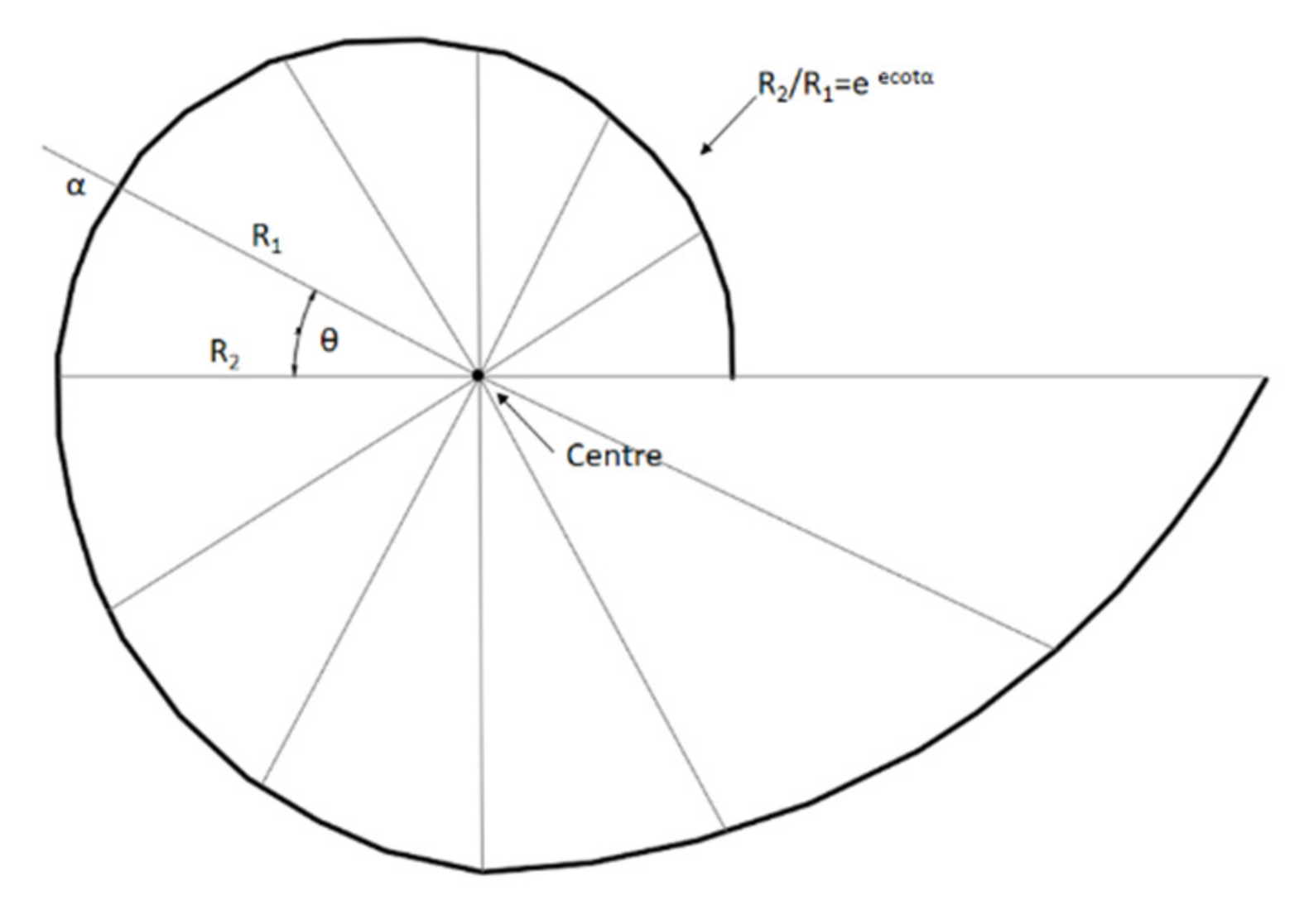
The logarithmic-spiral model was introduced by [12] observing an early 1940 imagery of Half-Moon Bay in California, USA. With field observations, the author realized that the bay adopted an equilibrium shape that is similar to a log-spiral. A definition sketch is given in Figure 1. The log-spiral equation, in polar coordinates, is given by:

$$R_1=R_2\exp \left(\theta cot\alpha \right)$$

(1)

where:

• R = Radius from origin
• θ = Angle between origin and R
• α = Constant angle of the tangent to the curve with radii R₁ and R₂

Despite of being the very first model proposed, representing a milestone in the field of crenulated bays research, the log-spiral model has long been criticized [3,23] because of several drawbacks which make it tricky to use. First, due to its constant curvature, the equation does not fit the relatively straight section of the headland bay beach; secondly, the pole of the log-spiral curve must be found by trial and error, because it does not coincide with the diffraction point, and could even deviate from it by a distance ranging from centimetres to kilometres (see [24]); therefore, it is not possible to predict the effect of relocating the headland (e.g., designing a headland bay beach introducing a coastal structure); and finally it does not take into account wave direction. In light of these disadvantages, two other empirical equations were developed: the hyperbolic-tangent equation and the parabolic equation.

The parabolic bay shape equation is a second-order polynomial equation developed by [15] and [16,17] in two separate works, from fitting the plan-shape of 27 mixed cases of prototype and model bays believed to be in static equilibrium:

$$\frac{R}{R_{\beta }}=C_0+C_1\left(\frac{\beta }{\theta }\right)+C_2{\left(\frac{\beta }{\theta }\right)}^2$$

(2)

where:

• $R_{\beta }$ = Control line length
• $R$ = Radius to a point along the curve at an angle θ
• $\beta$ = Wave obliquity
• $C$ = Constants generated by regression analysis
• $\theta$ = Angle between wave crest and radius to any point on the bay periphery

The two basic parameters are the reference wave obliquity β and control line length R_β (Figure 2). The variable β is a reference angle of wave obliquity, or the angle between the incident wave crest (assumed linear) and the control line, joining the upcoast diffraction point to a point on the near straight beach, namely the downcoast control point. The radius R to any point on the bay periphery in static equilibrium is angled θ from the same wave crest line radiating from the point of wave diffraction upcoast. The three C constants, generated by regression analysis to fit the peripheries of the 27 prototype and model bays, differ with reference angle β. Their analytical expressions have been provided by [14]:

$$C_0=0.0000000479{\beta }^4-0.00000879{\beta }^3+0.000352{\beta }^2-0.00479\beta +0.0715$$

(3)

$$C_1=-0.000000128{\beta }^4+0.0000182{\beta }^3-0.000487{\beta }^2+0.00771\beta +0.955$$

(4)

$$C_2=0.0000000944{\beta }^4-0.000012{\beta }^3+0.000316{\beta }^2-0.00828\beta +0.0265$$

(5)

In contrast to the log-spiral, the parabolic equation origin coincides with the diffraction point and therefore the equation is directly related to wave direction. However, it is affected by a drawback: the uncertainty of locating the downdrift control point. Despite that there are several interpretations of the downcoast control point of the parabolic bay shape equation [14], it is a considerable limitation which inhibits the application of the parabolic model in designing new beaches.

The hyperbolic-tangent shape model was derived by [13] through the analysis of 46 beaches around Spain and North America. Its equation is defined in a relative Cartesian coordinate system (Figure 3) as:

$$y=\pm atan{h}^m\left(bx\right)$$

(6)

where:

• $y$ = Distance across shore [m]
• $a$ = Empirically determined dimensional coefficient [m]
• $b$ = Empirically determined dimensional coefficient [1/m]
• $m$ = Empirically determined coefficient [dimensionless]
• $x$ = Distance alongshore [m]

The x-axis is parallel to the general trend of the shoreline while the y-axis points shoreward; the origin of the coordinates is placed at the point where the local tangent to the beach is perpendicular to the general trend of the shoreline. The hyperbolic tangent curve is symmetric with the x-axis and produces two asymptotes, found at $y=\pm a$. The line $y=+a$ indicates the location on the shoreline which is no longer under the influence of the headland. The parameter $a$ controls the magnitude of the asymptote (distance between the relative origin of coordinates and the location of the straight shoreline), $b$ is a scaling factor controlling the approach to the asymptotic limit and $m$ controls the curvature of the shape. These unknowns were found by using trial and error and an optimisation procedure that minimises rms errors. The authors of [13] found the following relationships: $ab\cong 1.2; m\cong 0.5$.

The model indirectly considers wave direction and, initially, it does not correlate the diffraction point with the origin of the hyperbolic tangent.

In 2018, [14] presented a development of the hyperbolic-tangent equation, establishing a relationship between the existing hyperbolic-tangent shape equation with the wave diffraction point. The authors used a database of case studies comprised of 46 beaches in Spain, Southern France and North-Africa, determining the coefficients a, b and m. The value of m is about 0.496, supporting the original findings of [13]. Moreover, the authors estimated a correlation between a and b, and the hyperbolic tangent shape equation became:

$$y=\pm atan{h}^{0.496}\left(1.794a^{-1.097}x\right)$$

(7)

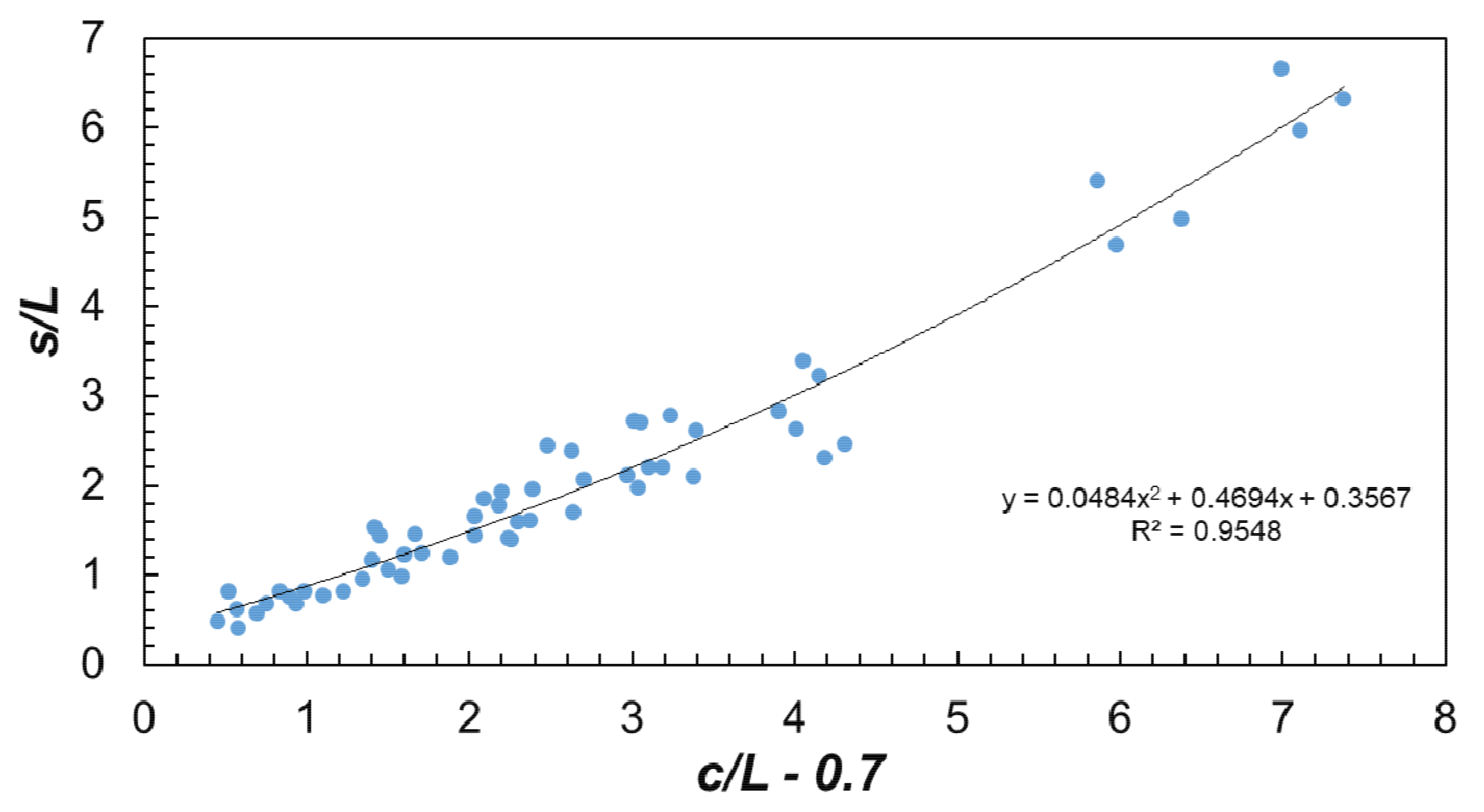
Overall, the research’s relevance has been constituted by two relationships which link the hyperbolic tangent profile and location of diffraction point. This makes the model easy to use, both in order to verify the bay’s stability and design a new beach. In the former case, starting from the distance between the location of diffraction point and asymptote, it is instantaneous to locate the origin of the equation and obtain the hyperbolic tangent profile; in the latter case, based on the shoreline advancement established in the illuminated zone, the location of the new diffraction point (i.e., new headland’s tip) can be directly carried out. The relationships, which correlate parameters c, d and a shown in Figure 4, are:

$$\frac{c}{a}=1.256$$

(8)

$$\frac{d}{a}=0.517$$

(9)

It is worth noting that the hyperbolic-tangent model could be applied not only to bay in static equilibrium conditions, but also to fit a bay under non-equilibrium conditions [3]. Among the three aforementioned models, the parabolic model prevailed over the others since it was the only one that used the wave diffraction point as the origin of the co-ordinate system, ensuring that the effect of relocating the diffraction point can be assessed [14]. Despite that, in comparing the origin of the three coordinates system in studying a headland bay (using a computer program based on a trial and error approach), [25] found that the parabolic equation’s origin was located in the middle of the ocean (Figure 5). This outcome weakens the strong point of parabolic model, revealing an uncertainty about its alleged robustness.

On the whole, regardless of models’ possible limitations, their description here presented shows how none of them model the relationship between wave characteristics and beach shape, but instead simply characterize the geometry of the headland bay profile. Nevertheless, over the last few decades, further investigations have been carried out towards the comprehension of the correlation between crenulate-shaped bays and wave characteristics. Particularly, several works focused on wave directional spreading, demonstrating that the crenulate-beach plan-form suffers under its influence. The authors of [26], searching for a new criterion to locate the downdrift control point of the parabolic shape equation, observed that the broader the directional spreading the farther the position of the downdrift control point. This behaviour indicates that, with a wider directional spreading of waves, a greater area could be influenced by wave diffraction behind the coastal structure (i.e., the transition zone increases).

During their numerical experimentation, [27] observed that a narrow directional spreading produces a more curved and asymmetric planform, confirming that the crenulated-beach behaviour is related to the modal directional spreading of incident waves [26,28]. Furthermore, [28] evaluated how the degree of directional spreading influences diffraction’s effect on the headland shape, observing that diffraction appears less important with a high directional spreading degree. The latter outcome is in accordance with [29], which demonstrated that diffraction shapes bay morphology only for wave climates with restricted approach angles.

Although important progress has been made, the effective correlation between wave forcing (i.e., diffraction and refraction) and static equilibrium profile has not been fully examined and understood. In this work we attempt to understand this issue, starting from the commonly engineering assumption that an equilibrium profile follows the wave front trend, with the aim of verifying the validity of this statement.

3. Numerical Experiments

The primary aim of this research is to investigate the relationship between the headland-bay static equilibrium profile and wave propagation characteristics; to do so, numerical modelling of a single headland case study has been implemented. Moreover, the possible influence of wave direction and wave period has been verified on this researched correlation. Several experiments have been carried out using the wave driver BW of MIKE 21 (Danish Hydraulic Institute) [21], which is based on the numerical solution of the time domain formulations of Boussinesq-type equations [30,31,32,33]. The BW module is able to reproduce the combined effects of all important wave phenomena, among them diffraction and refraction, which play an important role in headland-bay equilibrium profile shaping.

3.1. BW Model of MIKE 21 (DHI)

The Boussinesq model is capable of reproducing the combined effects of important wave phenomena, such as diffraction and refraction. Therefore, it has been used in numerical experimentation to obtain diffracted wave fronts generated by headland.

MIKE 21 BW includes two modules, the 2DH wave model and 1DH wave model, both based on the numerical solution of time domain formulations of Boussinesq-type equations, which are solved using a flux-formulation with improved linear dispersion characteristics. The enhanced Boussinesq equations were originally derived by [30,31], making the modules suitable for simulation of the propagation of directional wave trains travelling from deep to shallow water. Moreover, it contains wave breaking and moving shorelines, as described in [32,33,34]. The 2DH BW model has been used in this work.

The enhanced Boussinesq equations are expressed in terms of the free surface elevation, ξ, and the depth-integrated velocity-components, P and Q. The continuity and the momentum-conservation equations read:

$$n\frac{\partial \mathsf{\xi }}{\partial t}+\frac{\partial P}{\partial x}+\frac{\partial Q}{\partial y}=0$$

(10)

$$n\frac{\partial P}{\partial t}+\frac{\partial }{\partial x}\left(\frac{P^2}{h}\right)+\frac{\partial }{\partial y}\left(\frac{PQ}{h}\right)+\frac{\partial R_{xx}}{\partial x}+\frac{\partial R_{xy}}{\partial y}+n^{2}gh\frac{\partial \xi }{\partial x}+n^{2}P\left[\alpha +\beta \frac{\sqrt{P^2+Q^2}}{h}\right]+\frac{gP\sqrt{P^2+Q^2}}{h^2{C}^2}+n{\psi }_1=0$$

(11)

$$n\frac{\partial Q}{\partial t}+\frac{\partial }{\partial y}\left(\frac{Q^2}{h}\right)+\frac{\partial }{\partial x}\left(\frac{QP}{h}\right)+\frac{\partial R_{yy}}{\partial y}+\frac{\partial R_{yx}}{\partial x}+n^{2}gh\frac{\partial \xi }{\partial y}+n^{2}Q\left[\alpha +\beta \frac{\sqrt{P^2+Q^2}}{h}\right]+\frac{gQ\sqrt{P^2+Q^2}}{h^2{C}^2}+n{\psi }_2=0$$

(12)

with the dispersive Boussinesq terms ${\psi }_1$ and ${\psi }_2$, defined by:

$${\psi }_1=-\left(B+\frac{1}{3}\right)d^2\left(P_{xxt}+Q_{xyt}\right)-nBg{d}^3\left({\mathsf{\xi }}_{xxx}+{\mathsf{\xi }}_{xyy}\right)-d{d}_x\left(\frac{1}{3}{P}_{xt}+\frac{1}{6}{Q}_{xt}+ngBd\left(2{\mathsf{\xi }}_{xx}+{\mathsf{\xi }}_{yy}\right)\right)-d{d}_x\left(\frac{1}{6}{Q}_{xt}+ngBd{\mathsf{\xi }}_{xy}\right)$$

(13)

$${\psi }_2=-\left(B+\frac{1}{3}\right)d^2\left(P_{xyt}+Q_{yyt}\right)-nBg{d}^3\left({\mathsf{\xi }}_{xxy}+{\mathsf{\xi }}_{yyy}\right)-d{d}_x\left(\frac{1}{6}{P}_{xt}+\frac{1}{3}{Q}_{xt}+ngBd\left(2{\mathsf{\xi }}_{yy}+{\mathsf{\xi }}_{xx}\right)\right)-d{d}_x\left(\frac{1}{6}{P}_{yt}+ngBd{\mathsf{\xi }}_{xy}\right)$$

(14)

where d is the still water depth; g is the gravitational acceleration; n is the porosity; C is the Chezy resistence number; α is the resistance coefficient for laminar flow in porous media; β is the resistance coefficient for turbulent flow in porous media; B is the Boussinesq dispersion coefficient; the terms R_xx, R_xy and R_yy indicate the incorporation of the wave breaking by means of the surface roller model [35].

In MIKE 21 BW, the waves may either be specified along open boundaries or be generated internally within the model through the generation line; the latter must be placed in front of a sponge layer absorbing all outgoing waves. Moreover, porosity (e.g., to model partial transmission through porous structures) and sponge layers can be used on an ad hoc basis. At open boundaries, either a level boundary, namely wave energy given as time series of surface elevation, or flux boundary, where flux density is perpendicular to the boundary, can be set.

3.2. Methodology

The method followed involves comparing the diffracted wave fronts generated by the BW simulations with static equilibrium profiles sketched out by the hyperbolic-tangent model [13,14]. The procedure obeys to the following steps:

• generating the diffracted wave front through the BW module;
• extrapolating the wave front from the model;
• starting with the illuminated zone of the front, drawing out the hyperbolic-tangent profile.

The third step is directly related to one of the major findings in the field of static equilibrium bays, namely that equilibrium crenulated beaches tend to align transverse to the direction of dominant waves. The main assumptions in applying the methodology here proposed are that (1) the equilibrium headland-bay planform follows the wave front; and (2) that the predominant wave direction is perpendicular to the straight area of the bay. In this way, in order to obtain the hyperbolic tangent plan-form of every model configuration, we supposed that the asymptote of the hyperbolic tangent matches the illuminated zone of the wave front, out of the shadow zone where the influence of diffraction is negligible. Therefore, once the distance between asymptote and diffraction point is measured (distance c in Figure 5), the origin of the hyperbolic tangent is automatically obtained through Equations (8) and (9), and the x,y coordinates of hyperbolic tangent profile are achieved through Equation (7) (Figure 5). It is worth pointing out that, in order to compare equilibrium static profile and wave front, the latter must be able to expand without any kind of physical interference (e.g., presence of additional obstacles).

Additionally, in order to investigate the influence of wave characteristics on the relationship between wave fronts and equilibrium profiles, we performed different numerical simulation scenarios by varying wave direction, wave period and refraction conditions. For each scenario, more wave fronts were extrapolated from the BW module, each progressively further away from the headland tip, in order to examine the influence of dimensionless distance (c/L) on the researched correlation.

Finally, before describing the model set up, a clarification regarding the choice of the headland bay shape model is necessary. The two possible models to be implemented to sketch out the static equilibrium profile were the hyperbolic-tangent model [13,14] and the parabolic model [15,16,17,18] (the logarithmic spiral model [12] has been rejected a priori given its difficulty in practical application). Thus, the same methodology has been implemented to both the hyperbolic model and parabolic model. The results proved that there was no difference: there is no change, regardless of the model adopted. Nevertheless, given the uncertainty due to the determination of the downdrift control point of the parabolic profile, the hyperbolic tangent model [13,14] turned out to be the best static equilibrium model to be compared to the BW simulations wave fronts.

3.3. Boussinesq Wave Module Set Up

The primary aim of this research is to investigate the relationship between headland-bay static equilibrium profile and wave propagation characteristics (diffraction and refraction). Therefore, we created different numerical simulations scenarios, in order to generate different wave fronts, by varying wave direction, wave period and refraction conditions.

First, to evaluate refraction conditions, two bathymetry configurations were been investigated. The first one (called “gentle slope”) is characterised by a linearly varying cylindrical bathymetry, with a gentle bottom slope of 1/100 and a diffraction point, modelled through a breakwater, located at a water depth of 3 m. The water depth at the offshore boundary is 20 m (Figure 6a). A gentle slope has been adopted to allow an expansion of the wave fronts without the influence of bottom abrupt raising. The second configuration (called “flat bottom”) exhibits a bottom with a constant water depth equal to 10 m (Figure 6b).

Secondly, numerical experiments have been conducted considering the possible effect of wave period and wave direction; conversely, the influence of wave height was not explored. This is because the correlation function describing the relationship between static equilibrium profiles and wave characteristics, at this first stage of the research, is obtained through a “linear approach” based on simple geometric consideration. Therefore, the only parameters that could geometrically affect the aforementioned correlation are period, wave direction and bottom inhomogeneity. Conversely, wave height does not represent a variable of the problem. Three different wave directions have been investigated; one is normal to the breakwater, while the other two are angled of 25° and −35° with respect to being perpendicular to the structure. For each direction, three wave periods have been tested: 5.9 s, a typical wave period of the Mediterranean wave climate; and 10 s and 15 s, which simulate swell conditions. The wave height used was 0.8 m for each numerical scenario. Since the predominant wave shapes the crenulated beach, for the numerical experimentation the value of wave height has been chosen equal to the LDR equivalent wave height value for the case study of Bagnoli bay (see Section 5.2). Simulations have been implemented using regular waves. It is important to underline that the effect of breaking waves was not considered in the trials. For each bathymetry configuration (“gentle slope” and “flat bottom”), the scenarios analysed are summarized in

Table 1. Scenarios analysed in the numerical experimentation.

	Gentle Slope	Flat Bottom
Wave Direction	0°; 25°; −35°	0°; 25°; −35°
Wave Period	5.9 s; 10 s; 15 s	5.9 s

.

Models are made up of a fine grid (square cells with grid spacing 3 m), upon which orientation coincides with wave direction; the time step used is 0.1 s. The wave generation line has been used and wave absorbing sponge layers have been applied at the model boundaries. Near the land, one sponge layer has been applied in order to avoid the occurance of wave reflection which could influence the expansion of the wave fronts. Geometric characteristics are summarized in

Table 2. Grid geometric characteristics.

Grid Dimension [m2]	Grid Spacing [m]	Grid Orientation [°]	Headland Extension [m]
2100 × 1950	3	0	690
2700 × 1500	3	25	330
2700 × 1500	3	−35	630

, and are valid for both bottom configurations.

4. Results

At first sight, comparisons suggest that wave front does not represent a static equilibrium profile: within the shadow zone, the wave front is located backward from the static planform position, according to the wave propagation direction. In fact, as seen in Figure 7, the hyperbolic tangent profile (red line) crosses various fronts until it tends to the asymptote; the farther the asymptote from the breakwater tip, the more the profile is placed on additional wave fronts. On the other hand, wave fronts distant less than a wave length from the diffraction tip represent an exception, since they coincide with their corresponding hyperbolic tangent profile (Figure 8).

The behaviour outlined has been detected for each wave period and wave direction investigated, as shown in Figure 9. Moreover, this behaviour has been observed in both bottom configurations (gentle slope and flat bottom); consequently, it seems that the correlation between hyperbolic tangent profile and wave fronts is not influenced by the effect of refraction phenomenon. At the same time, although as a first approximation results indicate that wave front does not represent a static equilibrium profile, a more accurate inspection revealed that equilibrium beach profiles of single headland bays correspond to a simple translation of a wave front normal to the propagation line at the headland head: once shifted, it completely superimposes on the equilibrium profile (Figure 10). Specifically, this issue is elaborated and discussed in the next section.

Relationship between Wave Fronts and Equilibrium Profiles

As described in the above paragraph, numerical experiments demonstrated that, in contrast to what is usually supposed, wave fronts do not represent a static equilibrium profile. However, it is possible to establish a correlation between them. Regarding the fact that an equilibrium profile actually is a wave front translated perpendicularly to the wave direction at the headland head (Figure 10), and recognizing that wave period, wave direction and wave refraction do not influence this behaviour, it is possible to calculate a direct relationship between wave fronts and equilibrium profiles, called the “wave-front-bay-shape equation”.

Therefore, in order to derive this relationship, for each comparison between wave front and hyperbolic tangent profile, we measured the minimum distance between the diffraction point and the asymptote of the profile (distance c of Figure 10), and, also, the distance needed to overlap the front on the profile (distance s of Figure 10). These two distances have been standardised to the local wave length, L (the wave length at the diffraction point water depth), so obtaining c/L and s/L.

Moreover, it is necessary to take into account that wave fronts far from the diffraction point by less than one wave length coincide with the corresponding hyperbolic tangent profile. Therefore, it has been assumed that for a value of $c/L\le 0.7$, it is not necessary to shift the wave front to overlap it on the profile; they are already superimposed (Figure 8).

Hence, for each configuration, results have been plotted on a graph where on the x-axis there is “c/L − 0.7” and on the y-axis there is “s/L”. It can be noted that all results analysed tend to follow an increasing trend, which suggests that an equation to describe the correlation between diffractive wave fronts and static equilibrium profiles can be derived (Figure 11). The relationship is:

$$\frac{s}{L}=0.0484{\left(\frac{c}{L}-0.7\right)}^2+0.4694\left(\frac{c}{L}-0.7\right)+0.3567$$

(15)

with a correlation coefficient R² of 0.9548.

5. Bagnoli Bay Case Study

To assess the results carried out with numerical experiments, a small beach has been taken into account. It is located on the Bagnoli coast, West of Naples, in southern Italy (Figure 12). The beach is delimitated on the right (looking offshore) by a revetment which protects the road behind, on the left by a little mound and behind by a seawall which marks out the road; it extends for about 190 m from North-West to South-East. This little bay appears to be fundamentally governed by a single headland located on the left side, next to the drain of Bagnoli (Figure 13). The orientation of the downcoast section of the bay is approximately 210 °N and its distance from the diffraction point is approximately 47 m (Figure 13).

As will be demonstrated in the next section, the case study can be considered a static equilibrium bay governed by a single headland. For this reason, the application to the Bagnoli bay is of particular interest, as it allows us to verify the behaviour observed with numerical experimentation and to check the validity of Equation (15).

5.1. Wave Climate

The wave climate for the case study coast has been inferred from the MEDA-A buoy, an Acoustic Doppler Current Profile (ADCP), located approximately 800 m offshore from the bay (Figure 14a). The device is located at a depth of about 19 m below the low tide level, at a Latitude of 40°48.550′ N and a Longitude of 14°09.300′ E. Significant wave height, H_s, peak period, T_p, and azimuth of the mean wave direction, α, have been recorded in the period 2015–2018, with a large “white spot” interval detected, from 6 December 2016 to 22 March 2019. The histogram of wave direction for angular sectors of 22.5° N is shown in Figure 14b, where the offshore directed waves have been removed for sake of clearness. The graph exhibits how the bay is exposed to waves coming from a relatively narrow wave sector, included between 150 to 240° N, with a clear mode in the Southern quadrants (180°–210° N). It is important to highlight that, despite the short recorded time interval of the buoy (only three years), we employed its data, taking the advantage of being placed in the near-shore zone, bypassing all the procedures concerning the determination and propagation of the offshore wave climate (procedures which involve a certain degree of uncertainty, however).

5.2. LDR and Equivalent Wave

For the purposes of the present study, an understanding of longshore sediment transport is essential to sound headland control design practice, and for these scopes the concept of Littoral Drift Rose (LDR), [36,37] seems to represent a powerful resource. In fact, as stated previously, the long term sculpturing of headland bay beaches is related to the most persistent waves in their incidence and directions, since the straight section of the bay tends to lie normally to the wave rays. With minimizing the angle between dominant wave rays and the beach normal, the littoral drift progressively diminishes, so that the coast reaches its final equilibrium position. Therefore, such bays present their straight section normal to a dominant (or equivalent) sea state, embodied by the predominant swell on oceanic margins, and by the resultant energy vector in enclosed seas, where locally generated waves assume importance [5]. The LDR formulation is derived just from the energy vector concept [38], and, particularly, it holds the powerful property of estimating the climate equivalent (dominant) sea state, responsible for the sculpting of a stretch of coast; it is clear that it has a strong impact on the scopes of the article. Additionally, it is important to point out that, even though the equivalent wave concept is widely used in the field of practical coastal engineering, it lacks a firm theoretical basis. However, recent studies carried out by [39], demonstrated, through qualitative and quantitative analysis, how the equivalent wave concept may be reliable in explaining the long-term evolution of a stretch of coast. In light of this, the LDR for the case study area has been derived and the equivalent wave has been estimated and used as the wave attack that governs the plan-shape of the bay.

Now, as specified by [37], given a water climate represented by a series of N wave components, it is possible to determine the LDR, the compact polar representation of littoral transport potential for various shoreline orientations. For a segment of shoreline with outward normal azimuth β, it can be shown the net potential littoral drift rate, Q(β), can be calculated as:

$$Q\left(\beta \right)={{\displaystyle \sum }}_{{\alpha }_{0i}=\beta -\raisebox{1ex}{$\pi $}\!\left/ \!\raisebox{-1ex}{$2$}\right.}^{{\alpha }_{0i}=\beta +\raisebox{1ex}{$\pi $}\!\left/ \!\raisebox{-1ex}{$2$}\right.}{p}_i·\frac{K·{\left(H_{s0,i}\right)}^{2.4}·{\left(T_{p0,i}\right)}^{0.2}·g^{0.6}}{16·\left(s-1\right)·\left(1-n\right)·{\pi }^{0.2}} sin\left[2\left(\beta -{\alpha }_{0i}\right)\right]$$

(16)

In the equation above, Q is intended as the in-place volumetric transport of sediment past a hypothetical plane perpendicular to the beach; additionally:

• K is a sediment transport coefficient;
• g is gravity;
• s ≈ 2.6 is the ratio between the specific gravity of sediment and that of water;
• n ≈ 0.4 is the in place porosity;
• γ ≈ 0.6 is the breaker index (wave height to depth ratio);

As known, the LDR graph is a useful tool for interpreting littoral drift trends along a section of shoreline, and, more significantly, it is able to sum up the effects of the entire wave climate into a single equivalent wave component, of parameters H_s0,eq, T_p0,eq, α_0,eq. This is to say:

$$Q\left(\beta \right)={{\displaystyle \sum }}_{{\alpha }_{0i}=\beta -\raisebox{1ex}{$\pi $}\!\left/ \!\raisebox{-1ex}{$2$}\right.}^{{\alpha }_{0i}=\beta +\raisebox{1ex}{$\pi $}\!\left/ \!\raisebox{-1ex}{$2$}\right.}{p}_i·\frac{K·{\left(H_{s0,i}\right)}^{2.4}·{\left(T_{p0,i}\right)}^{0.2}·g^{0.6}}{16·\left(s-1\right)·\left(1-n\right)·{\pi }^{0.2}}\sin \left[2\left(\beta -{\alpha }_{0i}\right)\right]\cong G_{eq}·sin\left[2\left(\beta -{\alpha }_{0,eq}\right)\right]$$

(17)

where:

$$G_{eq}=\frac{K·{\left(H_{s0,eq}\right)}^{2.4}·{\left(T_{p0,eq}\right)}^{0.2}·g^{0.6}}{16·\left(s-1\right)·\left(1-n\right)·{\pi }^{0.2}}$$

(18)

The equivalent wave angle ${\alpha }_{0,eq}$, corresponds to the LDR node (null-point), as seen in Figure 15, and the magnitude (Equation (18)) can be easily inferred by using (for example) common harmonic regression techniques. The drift rose of Bagnoli bay has been derived using Equation (17) and the available wave data inferred through the MEDA-A Buoy. The range of shoreline orientations that exists at the site of interest has been also considered, and the net littoral drifts for each possible shoreline orientation have been calculated. LDR for the Bagnoli climate is shown in Figure 15: positive (transport to the right), and negative (transport to the left) lobes can be distinguished; moreover, the graph shows the null point; that is, the shoreline orientation at which no sediment transport is taking place.

From the LDR, the equivalent wave component parameters have been estimated according to Equation (17). The equivalent direction corresponds to the null-point of the real LDR (205° N for the present case), while H_s,eq and T_p,eq are fitted to have the same littoral transport magnitude, obtaining H_s,eq = 0.8 m and T_p,eq =5.89 s (Equation (18)). Additionally, it is worth noticing that, as explained by [39], in [37] the authors do not define explicitly how to derive the equivalent wave height and period. While the equivalent wave direction is much easier to interpret, as it corresponds to the null point of the LDR, the same is not true for H_s,eq, and T_eq. However, the equivalent wave height can be easily inferred from Equation (18), considering that a relationship between wave height and period is established. As such, the equivalent period can be considered as the spectral peak period T_p; in fact, assuming that the energy distribution is that of a mean-JONSWAP spectrum (typical spectrum shape of Mediterranean Sea), wave height and period are related by:

$$T_p=8.5\pi \sqrt{\frac{H_{m0}}{4\pi }}$$

(19)

On the other hand, the equivalent wave period can be considered as the “longer period” representative of swell-wave conditions. The authors of [40], in fact, argued the annual littoral transport to be driven by swells that follow the most intense storms and recognized that swells “arrive on a coast from persistent direction”. This implicitly supports the idea that a dominant swell-wave attack for shoreline evolution may exist. However, [11] claimed that the swell-wave predominance is more common for ocean margins rather than for enclosed or semi-enclosed seas, where, on the contrary, the swell-effect is minimum. In light of this, only the peak period T_p has been taken into account in the present study. However, further investigation on the effects of swell wave could be carried out and verified in future research works. In Figure 15, the Climate-LDR and Equivalent-LDR are compared.

It is surprising to observe that the equivalent wave direction (205° N) is extremely close to the orientation of the downcoast section of the bay (illuminated zone, Figure 13), confirming the results obtained in [37] that the LDR equivalent wave is responsible of the sculpturing of the bay, in the long run, bringing it to its static equilibrium plan-form. Moreover, this is confirmed also by the wave climate mode shown in Figure 14b: waves with the largest percentage of occurrence are those comprised within the south west wave sector, in which the 205° equivalent direction can be detected. In fact, it can be said that the LDR equivalent wave approximately represents the average climate; in other words, it is the wave component that usually affects a given region from a certain direction. Therefore, when in narrow wave sector, as the present case of Bagnoli bay, we are used to observe mono-modal wave climate, so with a single high-frequency direction. In such conditions, the directional mode corresponds to the average one, which corresponds, in turn, to the LDR equivalent wave direction [39].

5.3. Static Equilibrium Condition

Before moving on the application of the methodology exposed in the previous paragraphs to the case study, it has been verified that the bay under study is in a static equilibrium condition. Therefore, we analysed the shoreline position over 10 years, specifically from 2008 to 2018. Data comes from the digitalization, in QGIS environment, of historical imageries of the area from Google Earth (Figure 16a).

The Linear Regression Rate (LRR) and the End Point Rate (EPR) have been used as indicators of the rate of shoreline change. LRR corresponds to the slope of a least-square straight-line, fitted through the shoreline positions at the various available times; EPR, takes into account exclusively shoreline positions at the first and the last years concerned and represents shoreline movement during that time.

From the analysis of both LRR and EPR (Figure 16b), an erosive trend has been observed in the curved zone, meanwhile the linear stretch has been accreted. Therefore, this suggests that a long-shore transport occurs, which moves sediments from the shadow zone to the downcoast sector (illuminated zone). Nevertheless, the maximum rate of erosion and accretion are negligible, as they are approximatively 0.2 m/year and 0.4 m/year, respectively. Therefore, it can be asserted that the case study bay is in a static equilibrium condition.

6. Numerical Modelling of the Bay and Results

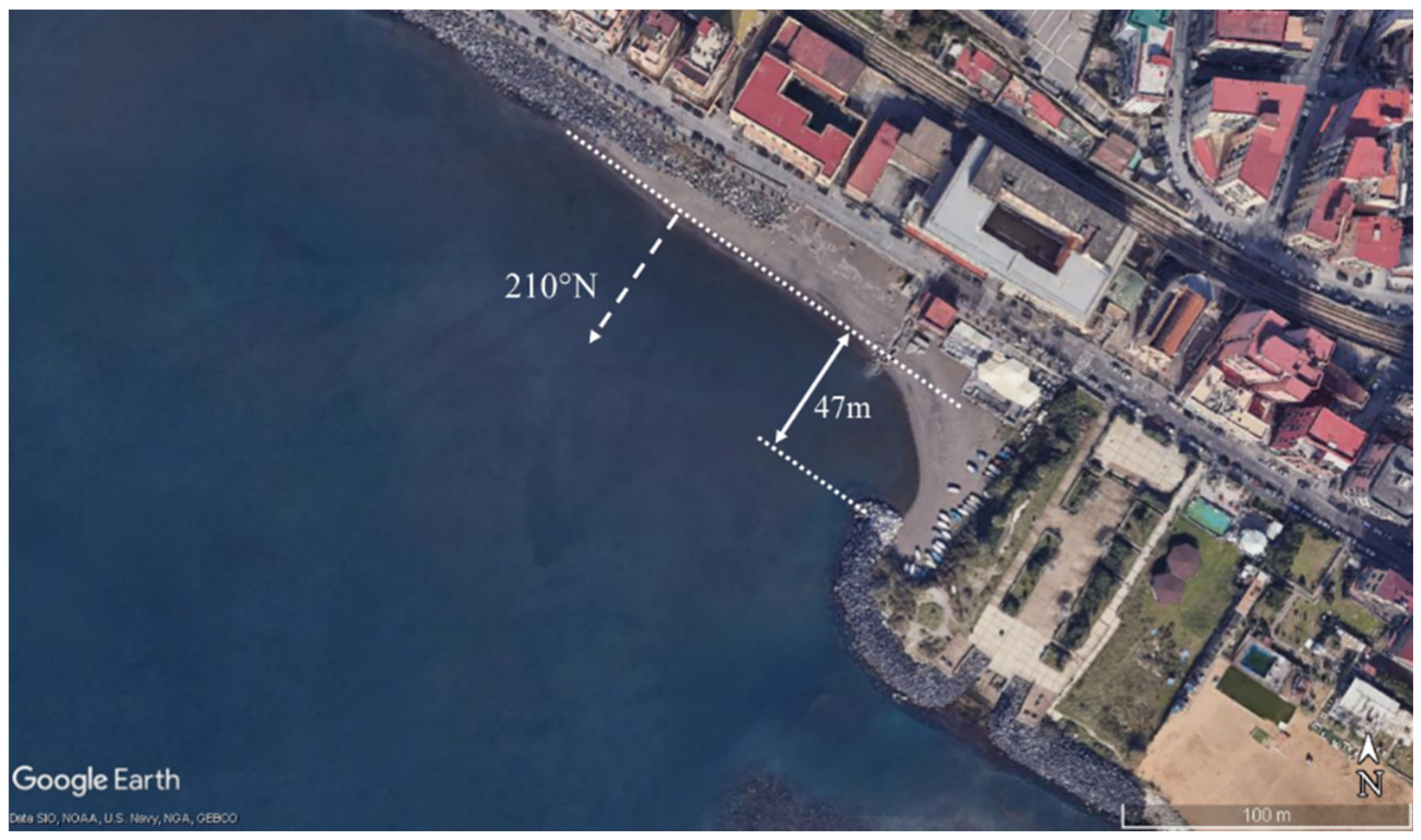
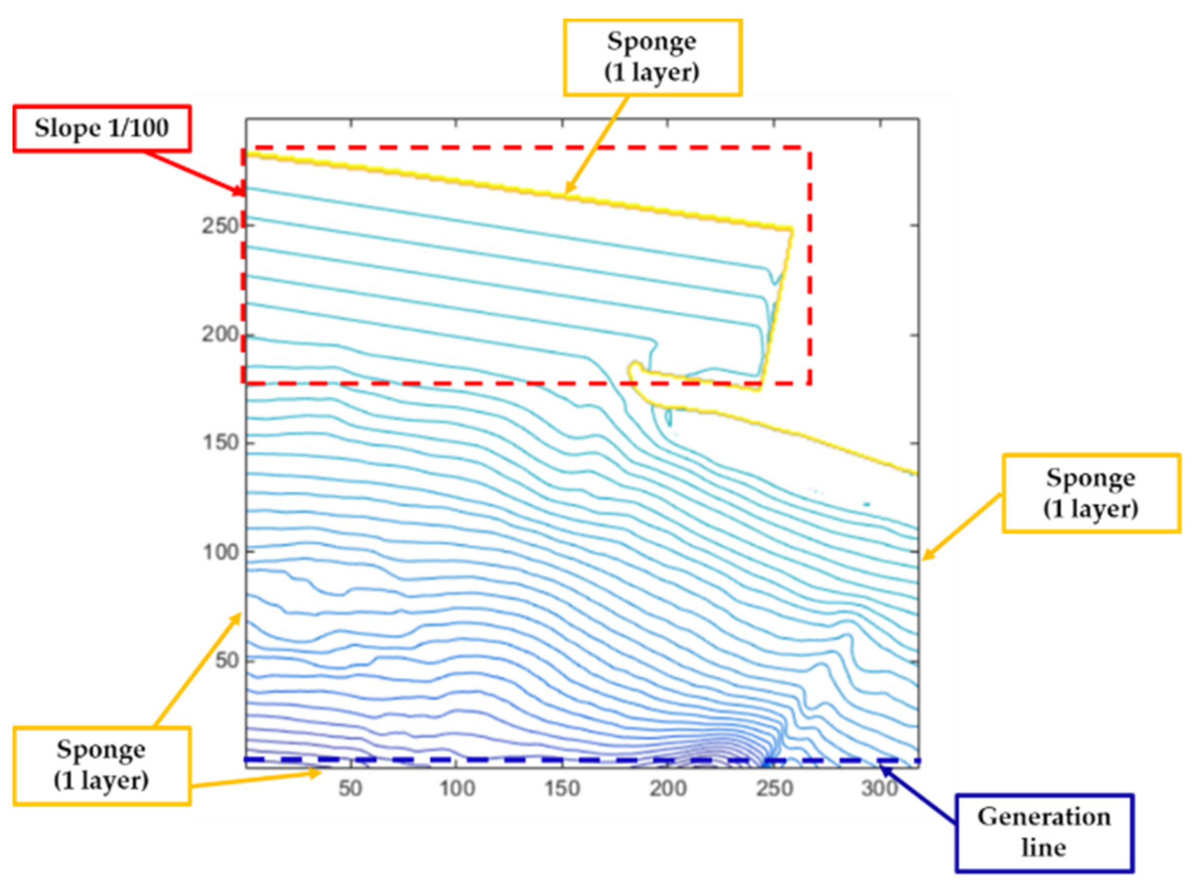
Numerical modelling of the bay has been performed through the wave driver MIKE 21 BW (DHI), which allows for obtaining the growth of the wave fronts leeward of the headland. In order to follow the method used in the numerical trial, the bay has been modelled in such a way that wave fronts could extend leeward the headland without any interference: the real bathymetry of the area has been employed until the diffraction point location, where the water depth is about 3 m, then a gentle slope of 1:100 has been adopted; the coastline has been shifted and cut landward and a sponge layer has been used, in order to avoid reflection phenomenon (Figure 17).

Numerical simulations have been performed wave detecting the equivalent direction of 205° N, since it is representative of the effects of the entire wave climate on long-shore sediment transport [41]. As concerns wave period, the average measured omni-directional peak period (5.9 s) has been investigated.

Simulations have been carried out using regular waves, which wave height has been set at 0.8m; the breaking phenomenon has been neglected. Fine grid has been used (square cells with grid spacing 3 m), for which the orientation coincides with wave direction, with a time step of 0.1. A wave generation line has been used and wave absorbing sponge layers have been applied at the lateral boundaries. Grid geometric characteristics are summarized in

Table 3. Grid geometric characteristics.

Grid Dimension [m2]	Grid Spacing [m]	Grid Orientation [° N]
900 × 960	3	205

.

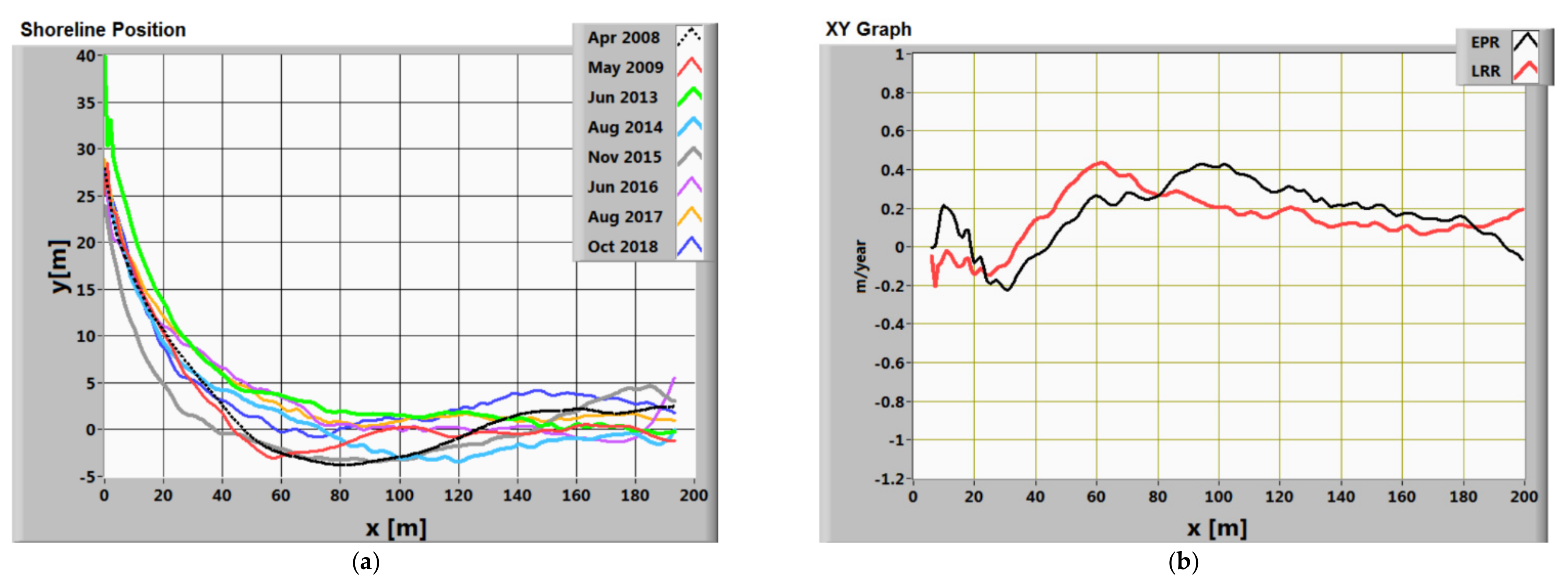
Comparison between equilibrium profile and wave fronts carried out through BW model, shown in Figure 18b, demonstrates that wave fronts’ direction in the illuminated zone matches shoreline orientation, confirming the goodness of the LDR equivalent wave to represent the entire wave climate in the act of shape the beach planform. Specifically, simulations results confirmed the behaviour observed in the previous section: the shoreline planform of the headland bay is placed on more wave fronts, the downdrift section overlaps the wave front while the curved section is placed on the wave front closer to the headland (Figure 18a).

In order to attain an effective validation of the wave-front-bay-shape equation, Equation (15) has been applied. The minimum distance between the diffraction point and the asymptote has been measured (distance c in Figure 19a) and it has been standardised with respect to the local wave length, c/L. Applying Equation (15), we obtained the value of the shift, s, which represents the distance needed to superimpose the whole wave front on the shoreline. After shifting the wave front, as shown in Figure 19b, it is perfectly superimposed on the bay shoreline, thus verifying the correlation found between wave fronts and shoreline profile, reached by Equation (15).

7. Conclusions

The main purpose of present paper is to establish a relationship between static equilibrium profiles of crenulated bays and wave front shapes and, more generally, understanding the correlation between bay shoreline response and wave forcings. The peculiar equilibrium plan-form (static or dynamic) of headland bays is assumed at a relatively long-term scale (e.g., annual to decadal) as a response to predominant wave direction; the downdrift segment of the bay, in fact, tends to align to the dominant direction of incoming waves, while, the curved up-coast segment is modelled by the diffracted wave fronts. In this regard, it is commonly believed by engineers that equilibrium beach profiles follow the wave front trend; however, this has been never fully proved so far. The most important works concerning headland bay beaches provided by the literature are empirical models, which simply describe the geometry of static equilibrium bays shape, neglecting the acting physical processes that sculpture the coast. In fact, they are merely of an empirical kind, lacking in a further insight on relationships between incident wave characteristics and beach shape. Therefore, in the lack of a model in which plan-shape is strongly correlated with wave characteristics, the project design of a new headland bay beach (necessary if the headland control practice has to be implemented) could, as a result, be extremely challenging.

To assess a possible correlation, numerical experiments have been carried out using the MIKE 21 Boussinesq Wave Module (BW), where wave fronts have been compared to the hyperbolic-tangent equilibrium profile, analysing the influence of wave direction, wave period and refraction phenomenon. Results proved that equilibrium profiles are located seaward compared to their relative wave fronts. Hence, designing a new beach following a wave front trends ensures a shoreline accretion in the sheltered zone (i.e., leeward to the headland). Additionally, a correspondence function, called the “wave-front-bay-shape equation” has been established, offering an easy application to engineering uses due to the simple geometric interpretation of its controlling parameters. The function seems to indicate that equilibrium beach profiles of a single headland bay correspond to a simple translation of wave front normal to the propagation line at the headland tip.

Moreover, the application of the “wave-front-bay-shape equation” to the case-study bay of the Bagnoli coast (south-west of Italy) has been performed. The numerical model has been set up, and the LDR equivalent wave concept has been used to embody the dominant wave attack that rules the long-term evolution of the little bay. Results confirm the behaviour observed from numerical experiments outcomes; the “wave-front-bay-shape equation” has been successfully verified, thus confirming that a correlation between equilibrium plan form and wave fronts can be found.

Nevertheless, the research still stands at a primary stage, and requires improvement and accurate verification in future research works in order to develop an enhanced guidance which could help in engineering and morphological practice.

References

1. Inman, D.L.; Nordstrom, C.E. On the Tectonic and Morphologic Classification of Coasts. J. Geol. 1971, 79, 1–21. [Google Scholar] [CrossRef]
2. Short, A.D.; Masselink, G. Embayed and structurally controlled beaches. In Handbook of Beach and Shoreface Morphodynamics; Short, A.D., Ed.; John Willey & Sons: Hoboken, NJ, USA, 1999; pp. 230–249. [Google Scholar]
3. Hsu, J.R.C.; Yu, M.J.; Lee, F.C.; Benedet, L. Static bay beach concept for scientists and engineers: A review. Coast. Eng. 2010, 57, 76–91. [Google Scholar] [CrossRef]
4. Silvester, R. Stabilization of sedimentary coastlines. Nature 1960, 188, 467–469. [Google Scholar] [CrossRef]
5. van der Meer, J.W.; Briganti, R.; Zanuttigh, B.; Wang, B. Wave transmission and reflection at low-crested structures: Design formulae, oblique wave attack and spectral change. Coast. Eng. 2005, 52, 915–929. [Google Scholar] [CrossRef]
6. Calabrese, M.; Buccino, M.; Pasanisi, F. Wave breaking macrofeatures on a submerged rubble mound breakwater. J. Hydro Environ. Res. 2008, 1, 216–225. [Google Scholar] [CrossRef]
7. Srisuwan, C.; Rattanamanee, P. Modeling of Seadome as artificial reefs for coastal wave attenuation. Ocean Eng. 2015, 103, 198–210. [Google Scholar] [CrossRef]
8. Buccino, M.; del Vita, I.; Calabrese, M. Engineering modeling of wave transmission of reef balls. J. Waterw. 2014, 140. [Google Scholar] [CrossRef]
9. Silvester, R.; Ho, S.K. Use of crenulate shaped bays to stabilize coasts. In Proceedings of the 13th International Conference on Coastal Engineering, Vancouver, BC, Canada, 10–14 July 1972; ASCE: Reston, VA, USA, 1972. [Google Scholar] [CrossRef]
10. Silvester, R.; Hsu, J.R.C. Coastal Stabilization: Innovative Concepts; Prentice-Hall: Englewood Cliffs, NJ, USA, 1993; p. 578. [Google Scholar]
11. Silvester, R. Coastal Engineering, 2nd ed.; Elsevier: Amsterdam, The Netherlands, 1974. [Google Scholar]
12. Krumbein, W.C. Shore processes and beach characteristics. In Technical Memorandum, vol. 3. Beach Erosion Board; U.S. Army Corps of Engineers: Washington, DC, USA, 1944; p. 47. [Google Scholar]
13. Moreno, L.J.; Kraus, N.C. Equilibrium shape of headland-bay beaches for engineering design. In Proceedings of the Coastal Sediments, New York, NY, USA, 21–23 June 1999; ASCE: Reston, VA, USA, 1999. [Google Scholar]
14. Kemp, J.; Vandeputte, B.; Eccleshall, T.; Simons, R.; Troch, P. A modified hyperbolic tangent equation to determine equilibrium shape of headland bay beaches. In Proceedings of the 13th International Conference on Coastal Engineering, Baltimore, MD, USA, 30 December 2018. [Google Scholar] [CrossRef] [Green Version]
15. Hsu, J.R.C.; Evans, C. Parabolic Bay Shapes and Applications. Proc. Inst. Civ. Eng. Part 2 1989, 87, 557–570. [Google Scholar] [CrossRef]
16. Hsu, J.R.; Silvester, R.; Xia, Y.M. Generalities on static equilibrium bays. Coast. Eng. 1989, 12, 353–369. [Google Scholar] [CrossRef]
17. Hsu, J.R.; Silvester, R.; Xia, Y.M. Static equilibrium bays: New relationships. J. Waterw. Port. Coast. Ocean Eng. 1989, 115, 285–298. [Google Scholar] [CrossRef]
18. Buccino, M.; Daliri, M.; Dentale, F.; Di Leo, A.; Calabrese, M. CFD experiments on a low crested sloping top caisson breakwater. Part 1. nature of loadings and global stability. Ocean Eng. 2019, 182, 259–282. [Google Scholar] [CrossRef]
19. Buccino, M.; Daliri, M.; Dentale, F.; Calabrese, M. CFD experiments on a low crested sloping top caisson breakwater. Part 2. Analysis of plume impact. Ocean Eng. 2019, 182, 345–357. [Google Scholar] [CrossRef]
20. Buccino, M.; Daliri, M.; Calabrese, M.; Somma, R. A numerical study of arsenic contamination at the Bagnoli bay seabed by a semi-anthropogenic source. Analysis of current regime. STOTEN 2021, 782, 146811. [Google Scholar]
21. MIKE 21 Boussinesq Wave Module. Available online: http://manuals.mikepoweredbydhi.help/2017/Coast_and_Sea/MIKE21BW_Sci_Doc.pdf (accessed on 3 October 2016).
22. Dingenmans, M.W. Water Wave Propagation over an Uneven Bottom; World Scientific: Singapore, 1997. [Google Scholar]
23. Benedet, L.; Klein, A.H.F.; Hsu, J.R.C. Practical insights and applicability of empirical bay shape equations. In Proceedings of the 29th International Conference on Coastal Engineering, Lisbon, Portugal, 19–24 September 2004. [Google Scholar] [CrossRef]
24. Yasso, W.E. Plan geometry of headland bay beaches. J. Geol. 1965, 73, 702–714. [Google Scholar] [CrossRef]
25. Martino, E.; Moreno, L.J.; Kraus, N.C. Engineering guidance for the use of bayed-beach formulations. In Proceedings of the Coastal sediments, Sheraton Sand Key Resort, Clearwater Beach, FL, USA, 18–23 May 2003; ASCE: Reston, VA, USA, 2003. [Google Scholar]
26. Elshinnawy, A.I.; Medina, R.; Gonzalez, M. On the influence of wave directional spreading on the equilibrium planform of embayed beaches. Coast. Eng. 2018, 133, 59–75. [Google Scholar] [CrossRef]
27. Castelle, B.; Robinet, A.; Idier, D.; D’Anna, M. Modelling of embayed beach equilibrium planform and rotation signal. Geomorphology 2020, 369, 107367. [Google Scholar] [CrossRef]
28. Hurst, M.D.; Barkwith, A.; Ellis, M.A.; Thomas, C.W.; Murray, A.B. Exploring the sensitivities of crenulate bay shorelines to wave climates using a new vector-based one-line model. J. Geophys. Res. Earth Surf. 2015, 120, 2586–2608. [Google Scholar] [CrossRef] [Green Version]
29. Daly, C.J.; Bryan, K.R.; Winter, C. Wave energy distribution and morphological development in and around the shadow zone of an embayed beach. Coast. Eng. 2014, 93, 40–54. [Google Scholar] [CrossRef]
30. Madsen, P.A.; Murray, R.; Sørensen, O.R. A new form of the Boussinesq equations with improved linear dispersion characteristics. Coast. Eng. 1991, 15, 371–388. [Google Scholar] [CrossRef]
31. Madsen, P.A.; Sørensen, O.R. A new form of the Boussinesq equations with improved linear dispersion characteristics. Part 2: A slowly-varying Bathymetry. Coast. Eng. 1992, 18, 183–204. [Google Scholar] [CrossRef]
32. Madsen, P.A.; Sørensen, O.R.; Schäffer, H.A. Surf zone dynamics simulated by a Boussinesq type model. Part I: Model description and cross-shore motion of regular waves. Coast. Eng. 1997, 32, 255–287. [Google Scholar] [CrossRef]
33. Madsen, P.A.; Sørensen, O.R.; Schäffer, H.A. Surf zone dynamics simulated by a Boussinesq type model. Part II: Surf beat and swash zone oscillations for wave groups and irregular waves. Coast. Eng. 1997, 32, 289–319. [Google Scholar] [CrossRef]
34. Sørensen, O.R.; Schäffer, H.A.; Sørensen, L.S. Boussinesq type modelling using unstructured finite element technique. Coast. Eng. 2004, 50, 181–198. [Google Scholar] [CrossRef]
35. Svendsen, I.A. Mass flux and undertow in a surf zone. Coast. Eng. 1984, 8, 347–365. [Google Scholar] [CrossRef]
36. Walton, T.L.; Dean, R.G. Application of littoral drift roses to coastal engineering problems. In Proceedings of the Conference on Engineering Dynamics in the Surf Zone, Sydney, Australia, 1 January 1973; Institution of Engineers: Sydney, VIC, Australia, 1973; pp. 221–227. [Google Scholar]
37. Walton, T.L.; Dean, R.G. Longshore sediment transport via littoral drift rose. Ocean Eng. 2010, 37, 228–235. [Google Scholar] [CrossRef]
38. US Army Corps of Engineers. Shore Protection Manual; Coastal Engineering Research Centre, Government Printing Office: Washington, DC, USA, 1984. [Google Scholar]
39. Di Paola, G.; Ciccaglione, M.C.; Buccino, M.; Rosskopf, C.M. Influence of hard defence structures on shoreline erosion along Molise coast (southern Italy): A preliminary investigation. Rend. Online Soci. Geol. Ital. 2020, 2–11. [Google Scholar] [CrossRef]
40. Silvester, R. Fluctuation in littoral drift. In Proceedings of the International Conference on Coastal Engineering, Houston, TX, USA, 3–7 September 1984; ASCE: Reston, VA, USA, 1984. [Google Scholar]
41. Buccino, M.; Di Paola, G.; Ciccaglione, M.C.; Del Giudice, G.; Rosskopf, C.M. A medium-term study of Molise coast evolution based on the one-line equation and “equivalent wave” concept. Water 2020, 12, 2831. [Google Scholar] [CrossRef]
Figure 1. Definition sketch for the log spiral.
Geosciences 11 00208 g001
Figure 2. Definition sketch for the parabolic equations.
Geosciences 11 00208 g002
Figure 3. Definition sketch for the hyperbolic-tangent shape equation.
Geosciences 11 00208 g003
Figure 4. Definition sketch of parameters for the modified hyperbolic-tangent equation.
Geosciences 11 00208 g004
Figure 5. Definition sketch to obtain the hyperbolic tangent profile starting from a wave front.
Geosciences 11 00208 g005
Figure 6. (a) Gentle slope configuration bathymetry; (b) flat bottom configuration bathymetry.
Geosciences 11 00208 g006
Figure 7. Comparison between wave front (obtained with flat bottom configuration) and hyperbolic tangent profile (red line), images from (ac) show profiles sketched out, starting with fronts gradually further from the headland.
Geosciences 11 00208 g007
Figure 8. Hyperbolic tangent profile (red line) corresponds to relative wave front; both pictures have been obtained with the gentle slope configuration, (a) with wave direction −35° and wave period of 10 s and (b) with wave direction 25° and wave period of 10 s.
Geosciences 11 00208 g008
Figure 9. Comparisons between wave fronts (black line) and hyperbolic tangent profiles (red line): (a) wave direction 0°, wave period 6 s, gentle slope configuration; (b) wave direction −35°, wave period 10s, gentle slope configuration; (c) wave direction −35°, wave period 6s, gentle slope configuration; (d) wave direction −35°, wave period 15 s, gentle slope configuration; (e) wave direction 25°, wave period 6 s, gentle slope configuration; (f) wave direction 25°, wave period 10 s, gentle slope configuration.
Geosciences 11 00208 g009
Figure 10. Definition sketch for parameters c (distance between the diffraction point and the asymptote of the profile) and s (distance needed to overlap the front on the profile).
Geosciences 11 00208 g010
Figure 11. numerical simulations values of s/L in function of c/L, together with the best line.
Geosciences 11 00208 g011
Figure 12. Location of the Bagnoli bay case of study.
Geosciences 11 00208 g012
Figure 13. Distance from diffraction point and shoreline orientation in downdrift section of the Bagnoli bay case study.
Geosciences 11 00208 g013
Figure 14. (a) Location of the MEDA-A buoy; (b) histogram of wave direction for angular sectors of 22.5° N.
Geosciences 11 00208 g014
Figure 15. Comparison between Climate-LDR and Equivalent-LDR of the Bagnoli bay; blue solid line represents drift to right when looking offshore, while red solid line represents drift to left when looking offshore; dashed lobes represent the equivalent drifts. Littoral drift in cubic meters/s.
Geosciences 11 00208 g015
Figure 16. (a) y(x,t) coordinates of shorelines over time; (b) EPR (black line) and LRR (red line).
Geosciences 11 00208 g016
Figure 17. Model setup of case study bay.
Geosciences 11 00208 g017
Figure 18. (a) Wave fronts generated by means BW; (b) comparisons between wave fronts (green lines) and shoreline (red line).
Geosciences 11 00208 g018
Figure 19. (a) Wave front (green line) that overlaps the shoreline (red line) in the downdrift section and the latter’s distance, c, from the diffraction point; (b) wave front shifted by s, which was derived from Equation (15).
Geosciences 11 00208 g019