Author Contributions
Conceptualization, X.Z. and C.X.; methodology, X.Z.; software, X.Z. and B.C.; validation, J.X., B.C. and Y.M.; formal analysis, X.Z.; investigation, X.Z. and B.C.; resources, X.Z. and Y.M.; data curation, X.Z.; writing—original draft preparation, X.Z.; writing—review and editing, X.Z.; visualization, X.Z.; supervision, C.X. and J.X.; project administration, C.X. and Y.M.; funding acquisition, C.X. and Y.M. All authors have read and agreed to the published version of the manuscript.
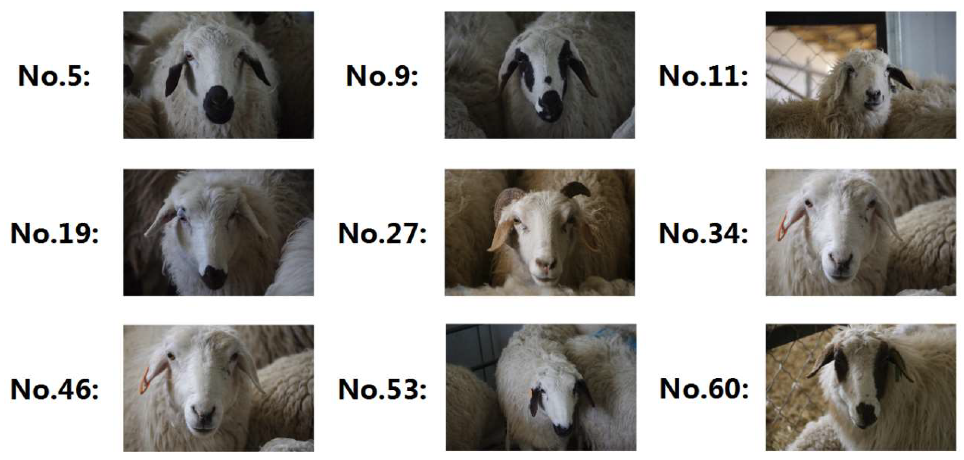
Figure 1.
Randomly selected examples of experimental sheep.
Figure 1.
Randomly selected examples of experimental sheep.
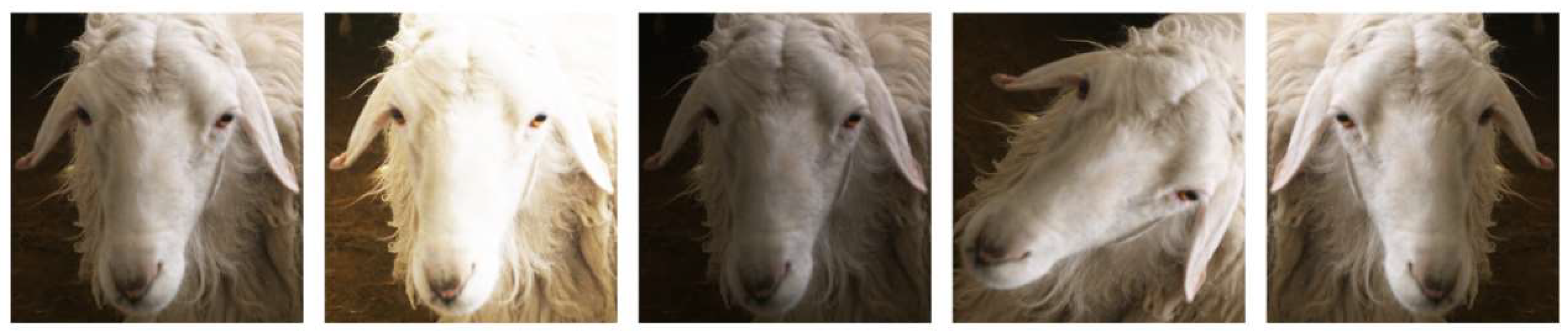
Figure 2.
The corresponding operations, from left to right, are the original image, brightened image, darkened image, image randomly rotated, and image vertically flipped.
Figure 2.
The corresponding operations, from left to right, are the original image, brightened image, darkened image, image randomly rotated, and image vertically flipped.
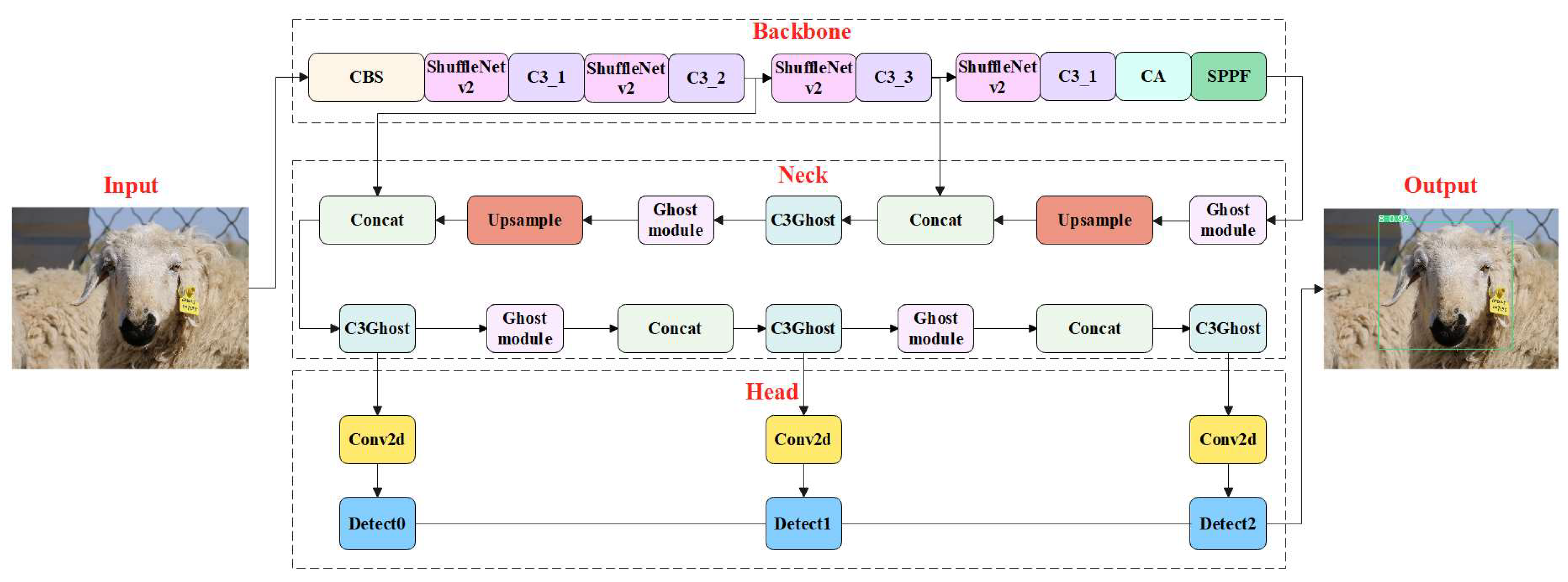
Figure 3.
Schematic diagram of LSR-YOLO. LSR-YOLO mainly includes the backbone, neck, and head, with lightweight ShuffleNetv2 module (pink) and attention mechanism CA module (cyan) added to the backbone. In the neck, the model size and parameters were further reduced by introducing the Ghost module (light pink) and C3Ghost module (light cyan).
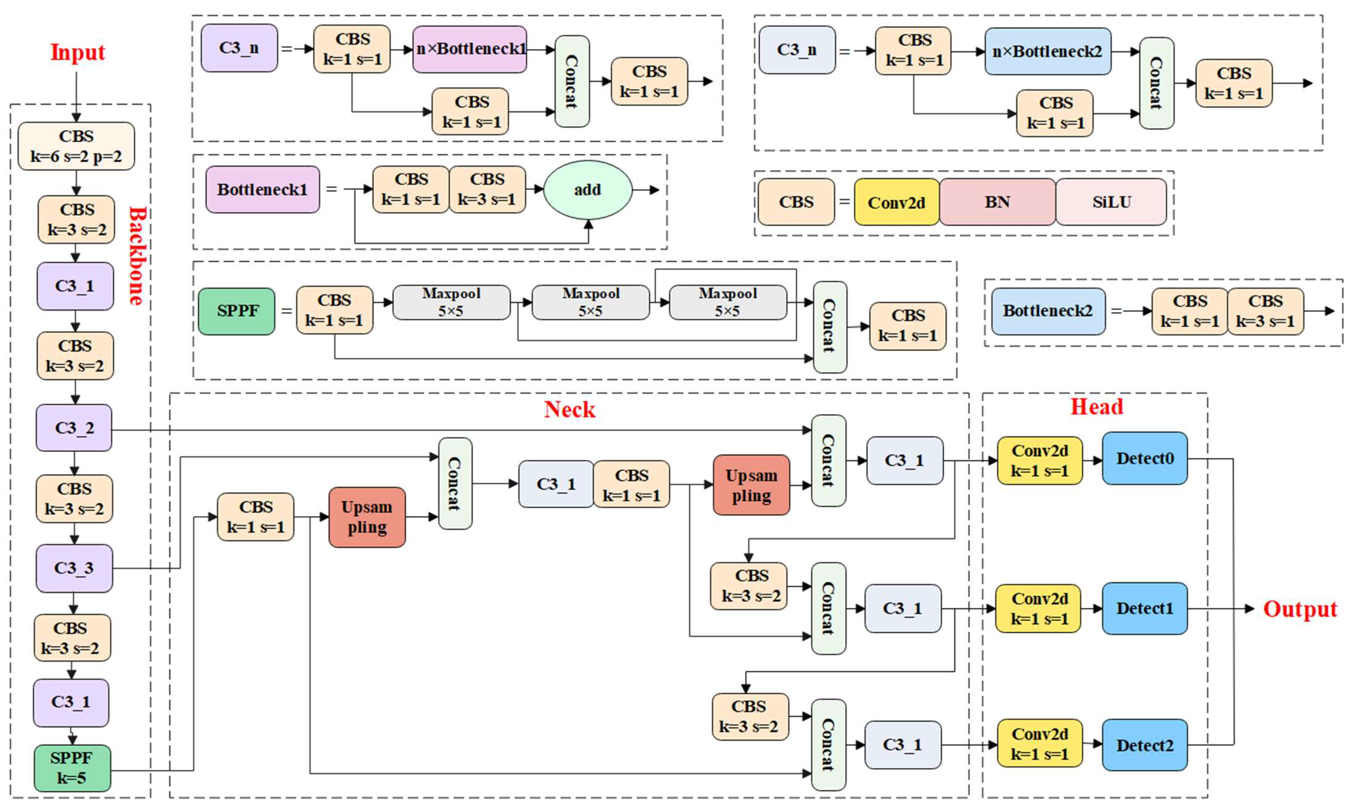
Figure 4.
Architecture diagram of YOLOv5s. CBS (orange) is the basic component module of YOLOv5s, used to extract target features. In the backbone, detailed target features are extracted through the C3P1 module (purple), and finally feature fusion is performed through the SPPF module (green). The CSP2 module (light gray) is used in the neck to extract target features. In addition, Upsampling operation (red) and Concat operation (light green) were also used in the neck. The head consists of three Conv2d modules (yellow) and three detection heads (blue).
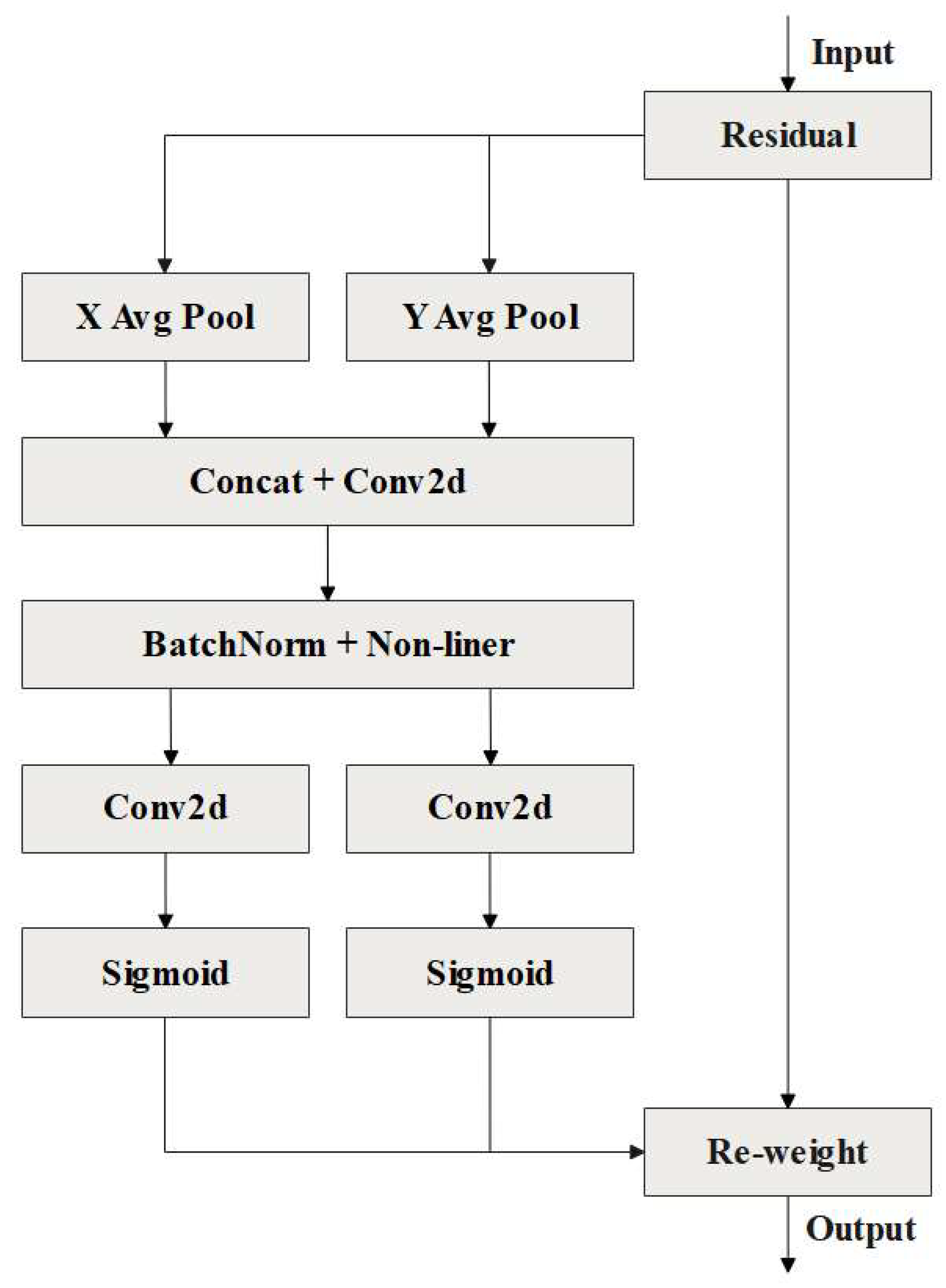
Figure 5.
Structure diagram of the CA attention mechanism.
Figure 5.
Structure diagram of the CA attention mechanism.
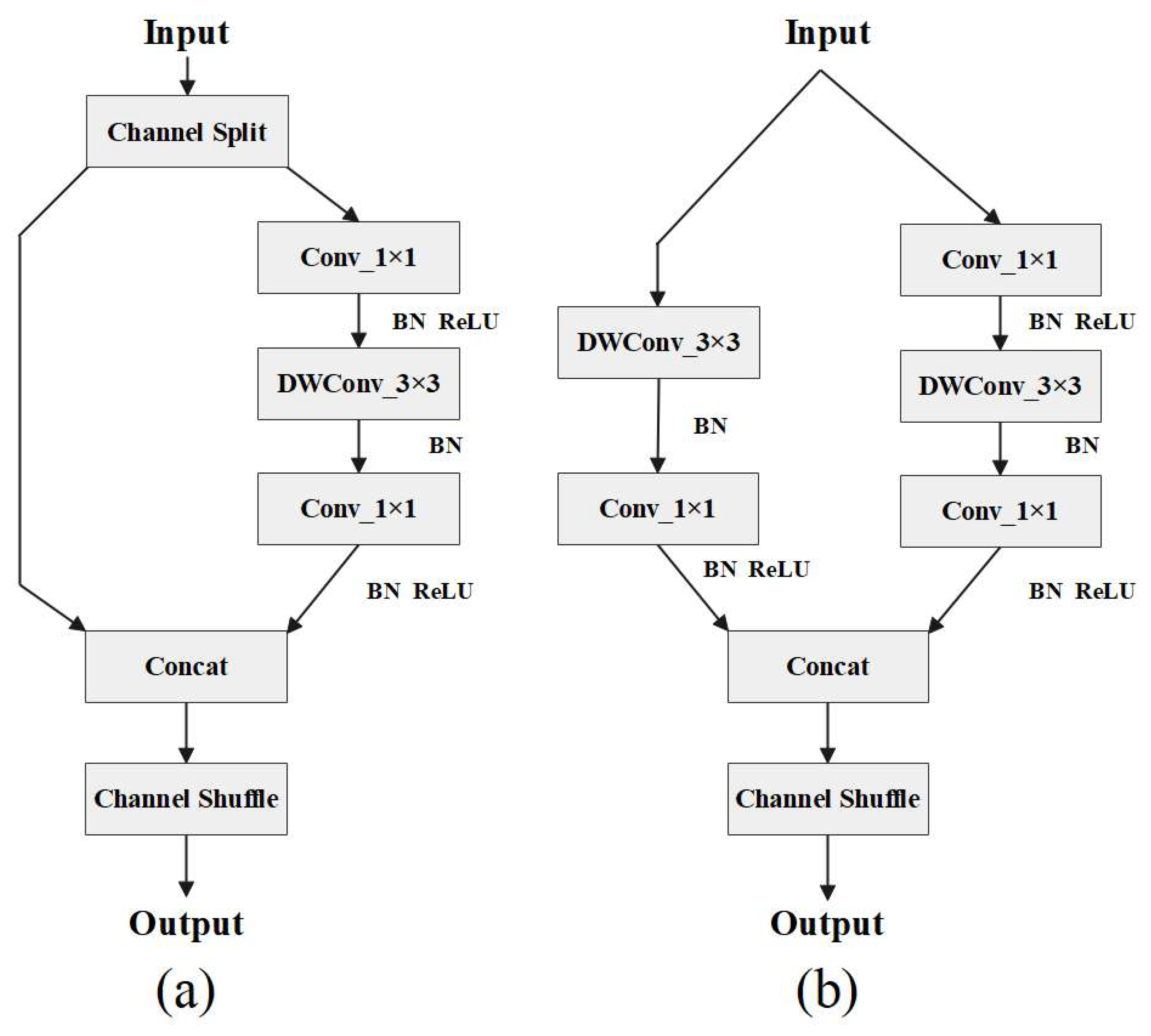
Figure 6.
(a) is the network structure diagram of ShuffleNetv2 when the stride is 1, and (b) is the structure diagram of ShuffleNetv2 when the stride is 2.
Figure 6.
(a) is the network structure diagram of ShuffleNetv2 when the stride is 1, and (b) is the structure diagram of ShuffleNetv2 when the stride is 2.
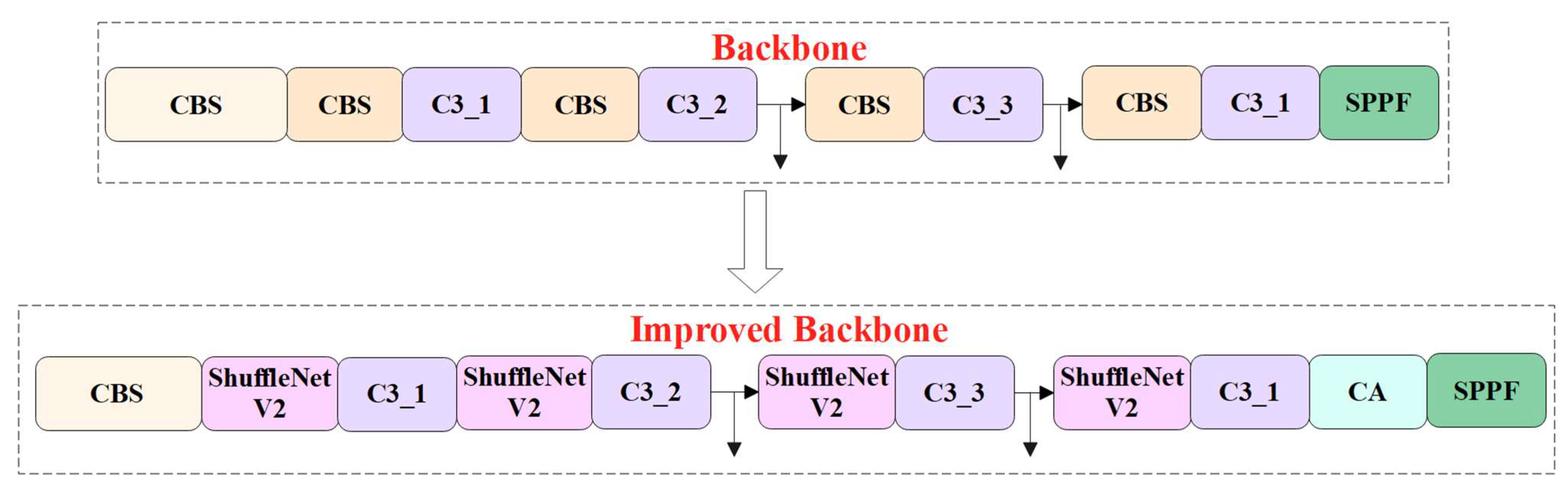
Figure 7.
Schematic diagram of the optimized backbone network.
Figure 7.
Schematic diagram of the optimized backbone network.
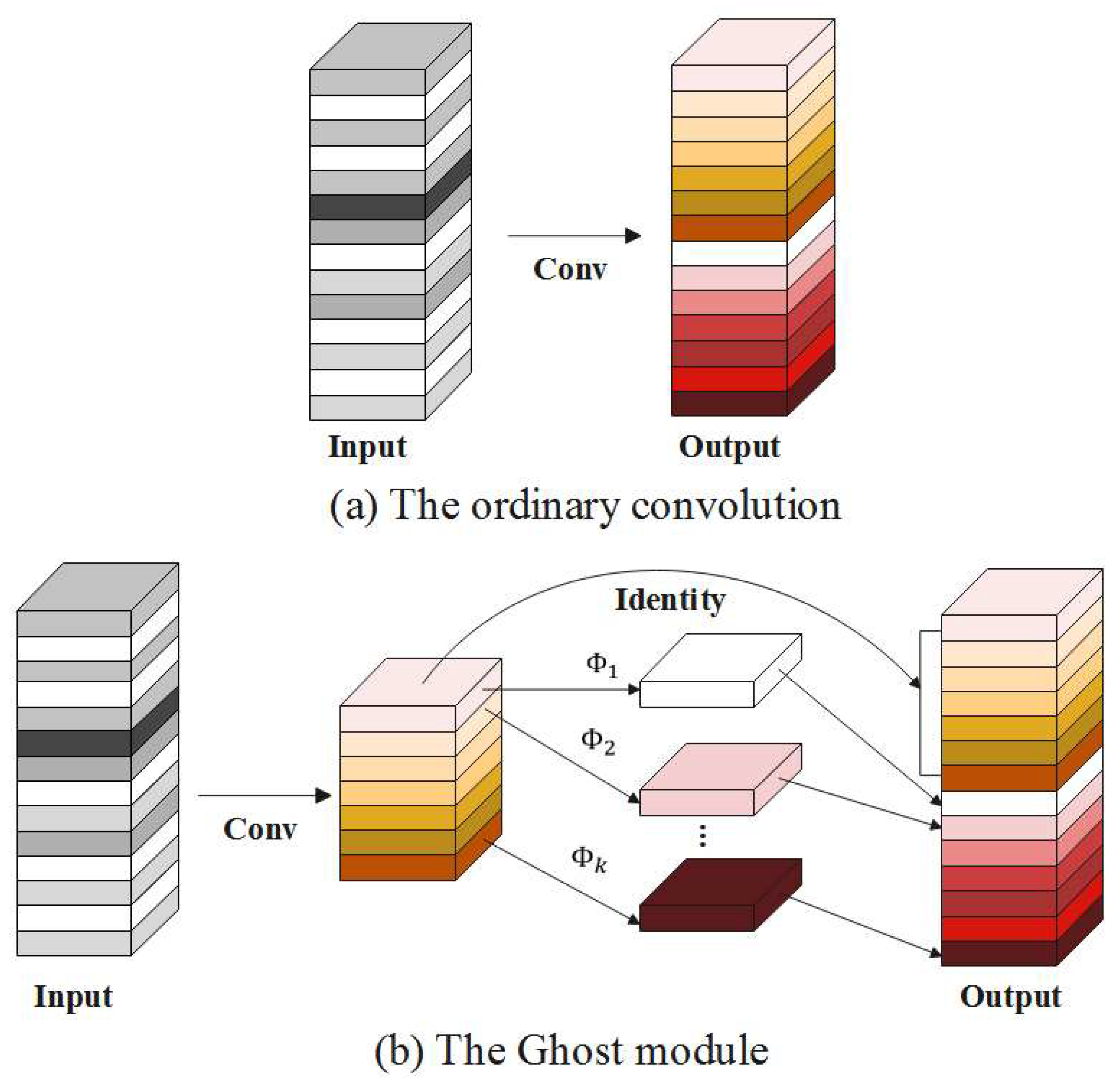
Figure 8.
Schematic diagrams of ordinary convolution and the Ghost module. (a) is the operation flow of traditional convolution. Suppose that is the size of the input feature map, and the convolution kernel is , where is the number of input channels, is the width of input data, and is the height of input data. The size of the output feature map is , where and are the width and height of the output feature map, and represents the number of output feature maps. The FLOPs of ordinary convolution can be calculated as . (b) is the Ghost module, which consists of two parts, including one part of ordinary convolution and the other part of the linear operation with less computation and fewer parameters. Through ordinary convolution, a total of feature maps are obtained. After linear operation, a total of new feature maps are generated from feature maps, and the two sets of feature maps are spliced in a specified dimension. Finally, a total of feature maps are generated in the Ghost module, and the size of the convolution kernel for each linear operation is . The FLOPs of the Ghost module can be calculated as .
![Animals 13 01824 g008]()
Figure 9.
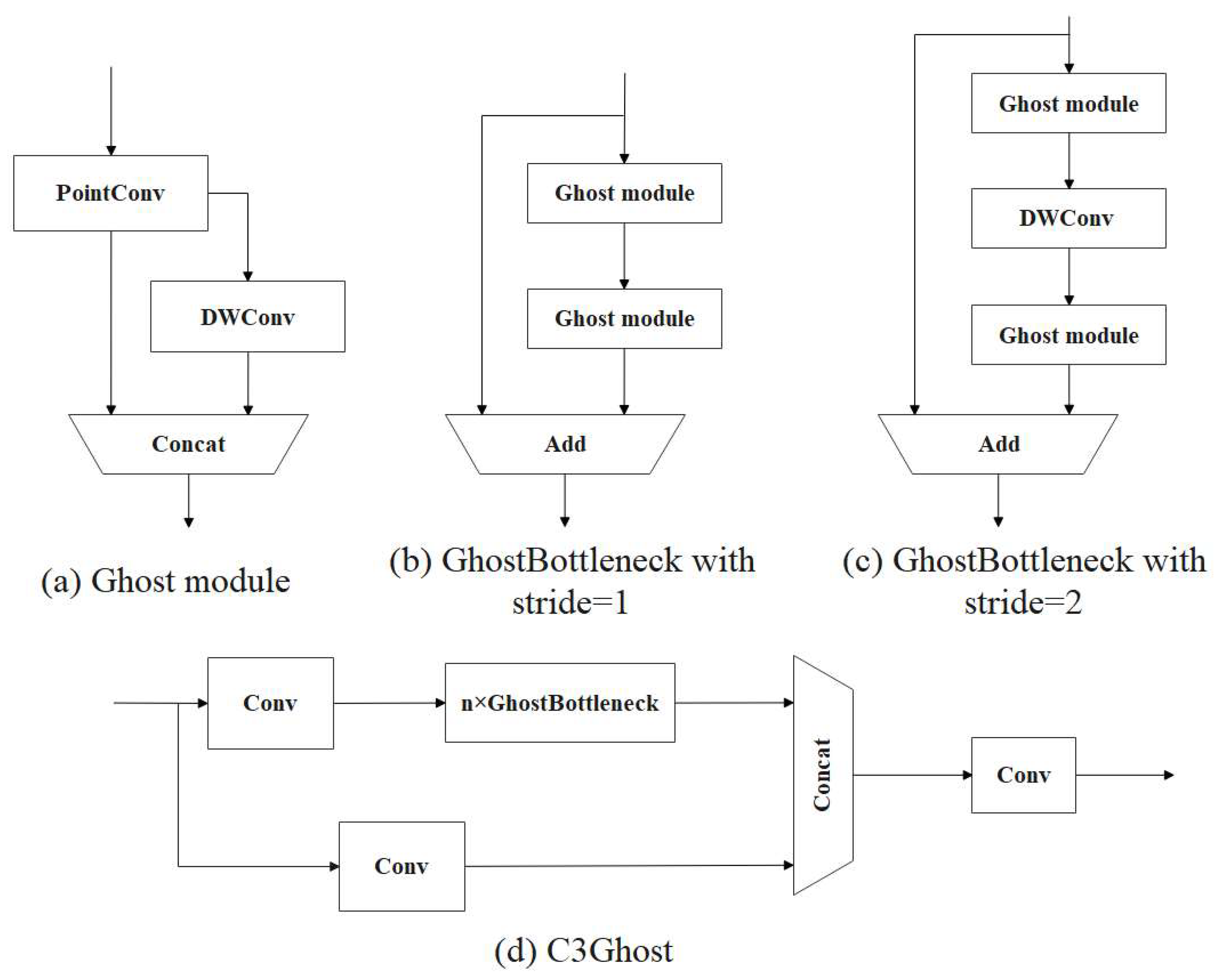
The specific structures of Ghost, GhostBottleneck, and C3Ghost. (a) is the structural diagram of Ghost module. The number of channels of the Ghost module is reduced to ½ of the number of output channels by 1 × 1 ordinary convolution. Then, a 5 × 5 DWConv is performed on the obtained feature map, and finally, the two sets of features are spliced. (b) is the structural diagram of the Ghost Bottleneck when the stride is 1. The Ghost Bottleneck consists of two stacked ghost modules. The first Ghost module is used for an extension layer that increases the number of channels. To match the number of channels for the input feature, the second Ghost module is used to reduce the number of channels. When the stride is 1, the two Ghost modules are directly performed, and then the input features and the output of the feature from the two Ghost modules are added for feature fusion. (c) is the structural diagram of the Ghost Bottleneck when the stride is 2. On the basis of the Ghost Bottleneck when the stride is 1, a DWConv with a step size of 2 is inserted between the two Ghost modules for downsampling. (d) is the structural diagram of C3Ghost module. The Bottleneck module in the C3 module is replaced with Ghost Bottleneck to form a C3Ghost structure. The new structure reduces the FLOPs and model size by replacing the 3 × 3 standard convolution in the original Bottleneck module.
Figure 9.
The specific structures of Ghost, GhostBottleneck, and C3Ghost. (a) is the structural diagram of Ghost module. The number of channels of the Ghost module is reduced to ½ of the number of output channels by 1 × 1 ordinary convolution. Then, a 5 × 5 DWConv is performed on the obtained feature map, and finally, the two sets of features are spliced. (b) is the structural diagram of the Ghost Bottleneck when the stride is 1. The Ghost Bottleneck consists of two stacked ghost modules. The first Ghost module is used for an extension layer that increases the number of channels. To match the number of channels for the input feature, the second Ghost module is used to reduce the number of channels. When the stride is 1, the two Ghost modules are directly performed, and then the input features and the output of the feature from the two Ghost modules are added for feature fusion. (c) is the structural diagram of the Ghost Bottleneck when the stride is 2. On the basis of the Ghost Bottleneck when the stride is 1, a DWConv with a step size of 2 is inserted between the two Ghost modules for downsampling. (d) is the structural diagram of C3Ghost module. The Bottleneck module in the C3 module is replaced with Ghost Bottleneck to form a C3Ghost structure. The new structure reduces the FLOPs and model size by replacing the 3 × 3 standard convolution in the original Bottleneck module.
![Animals 13 01824 g009]()
Figure 10.
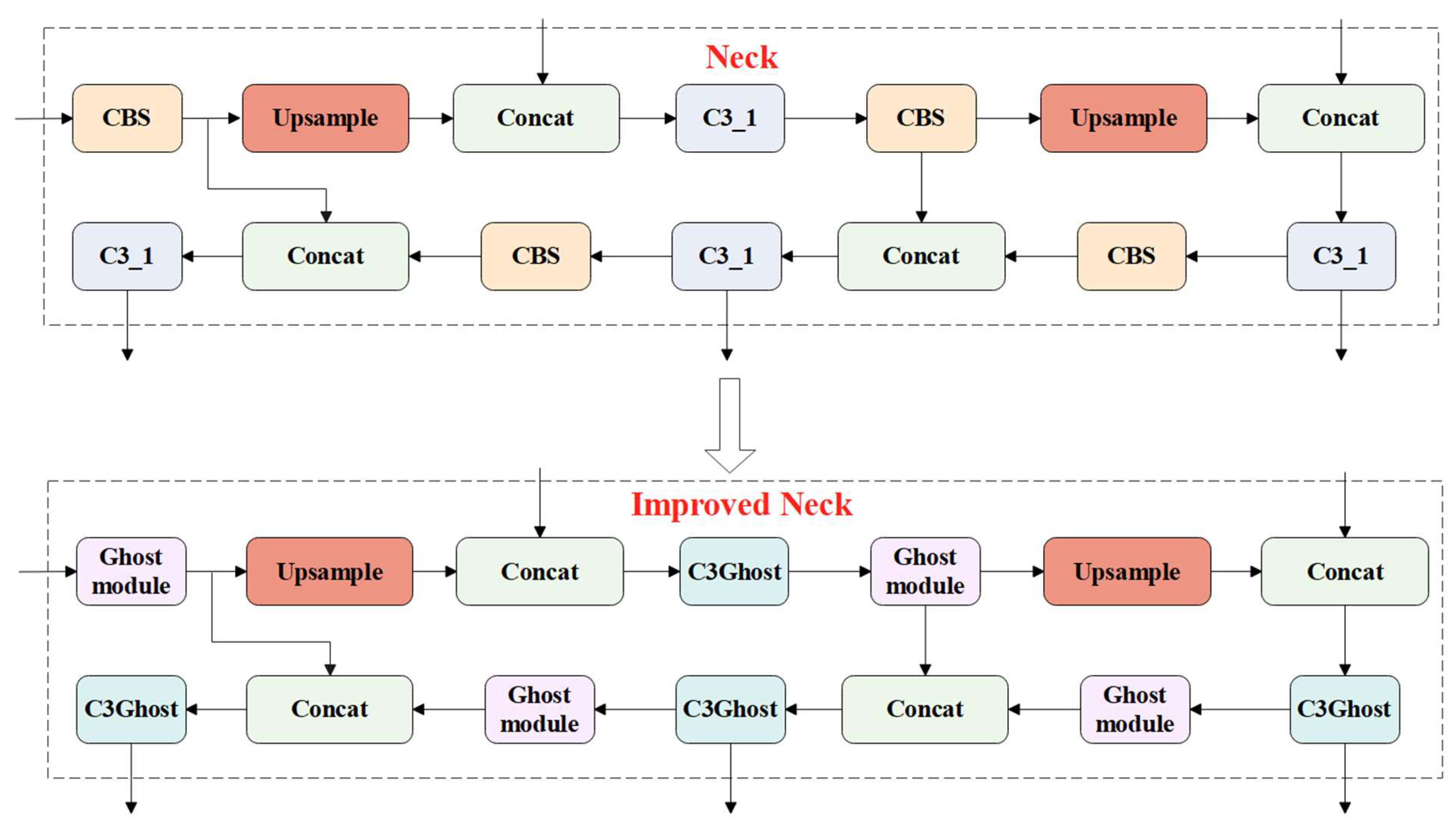
Schematic diagram of the improved neck network.
Figure 10.
Schematic diagram of the improved neck network.
Figure 11.
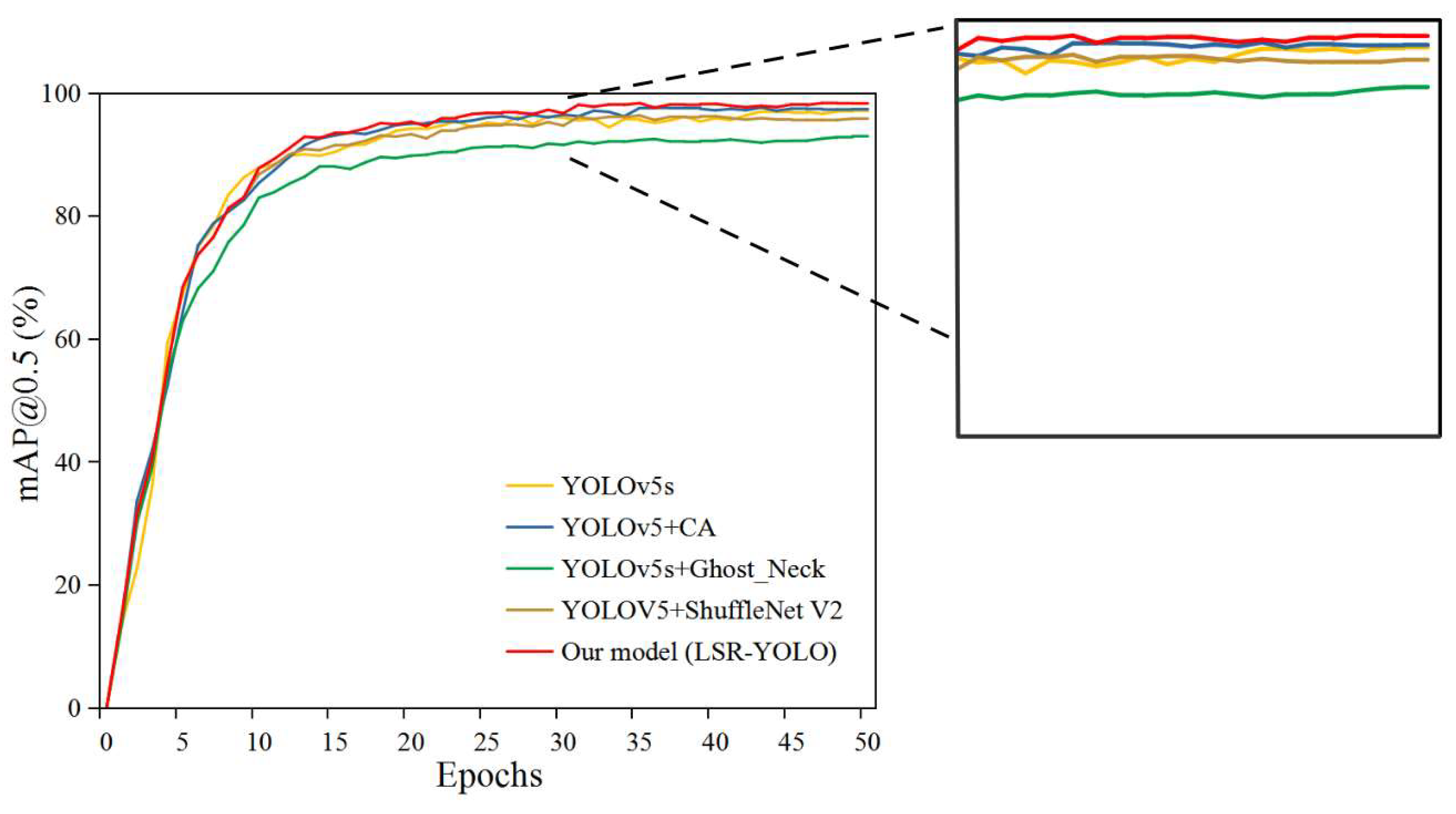
Training curves of multiple groups of improved models.
Figure 11.
Training curves of multiple groups of improved models.
Figure 12.
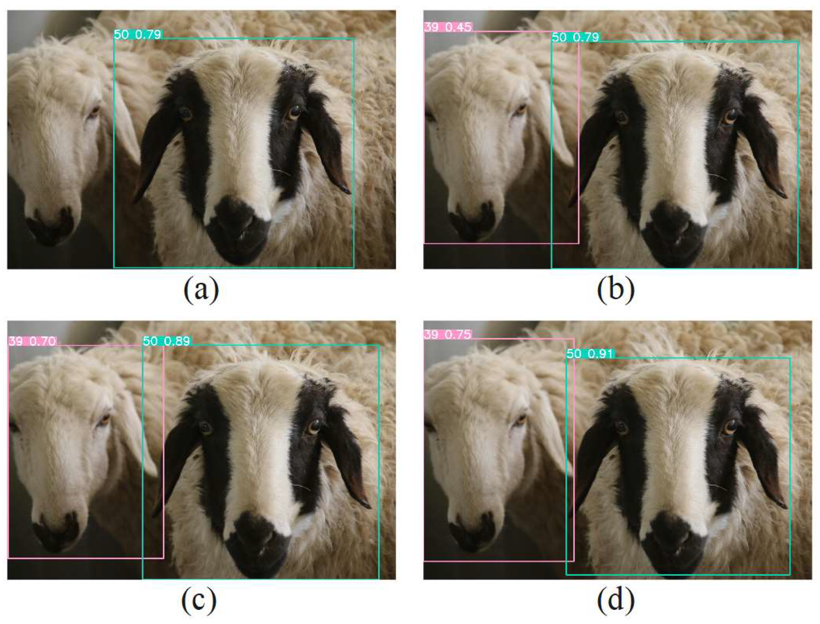
Recognition results of different improved models, including (a) the YOLOv5s + Ghost_Neck model, (b) the YOLOv5s model, (c) the YOLOv5s + CA model, and (d) the LSR-YOLO model. For different recognition targets, the model marks recognition boxes with different colors, and the colors of the recognition boxes are random.
Figure 12.
Recognition results of different improved models, including (a) the YOLOv5s + Ghost_Neck model, (b) the YOLOv5s model, (c) the YOLOv5s + CA model, and (d) the LSR-YOLO model. For different recognition targets, the model marks recognition boxes with different colors, and the colors of the recognition boxes are random.
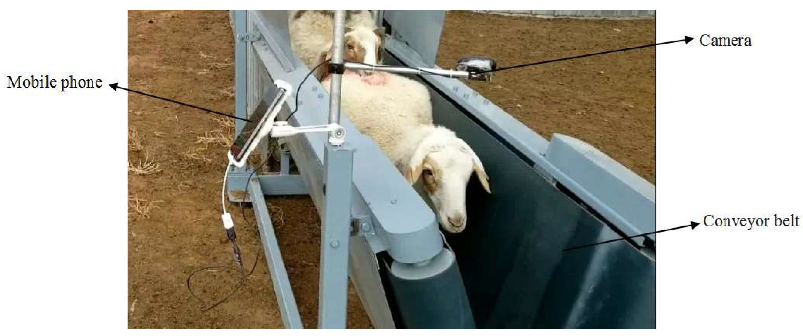
Figure 13.
The sheep facial image acquisition device.
Figure 13.
The sheep facial image acquisition device.
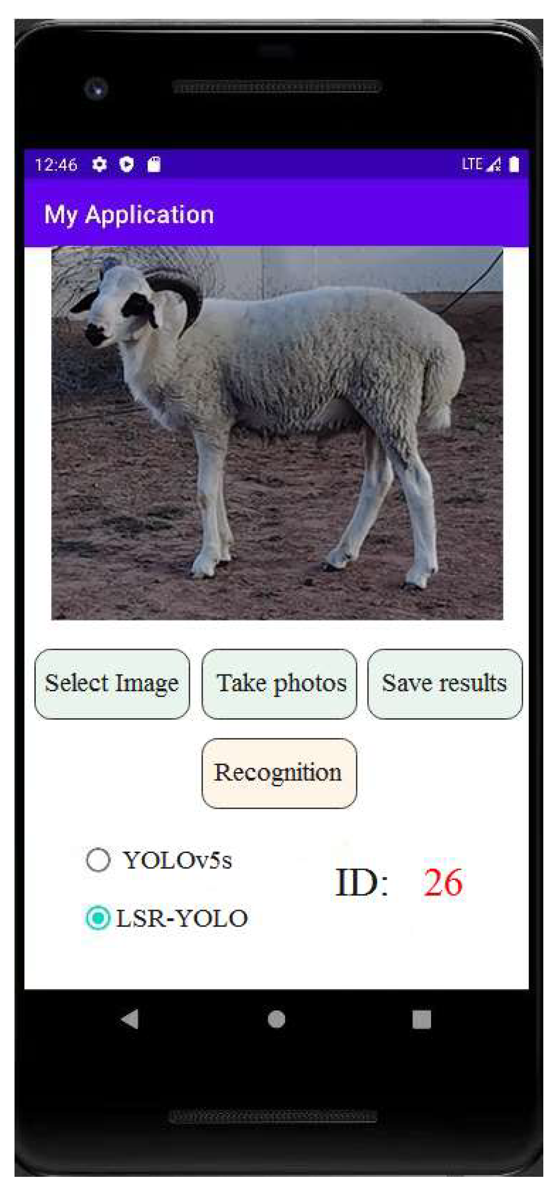
Figure 14.
Interface of the mobile sheep face recognition system.
Figure 14.
Interface of the mobile sheep face recognition system.
Table 1.
Specifications of the sheep face dataset.
Table 1.
Specifications of the sheep face dataset.
| Dataset | Images | Size | Proportion |
|---|
| Training | 9928 | 2736 × 1824 | 80% |
| Verification | 1241 | 2736 × 1824 | 10% |
| Testing | 1241 | 2736 × 1824 | 10% |
| Total | 12,410 | 2736 × 1824 | 100% |
Table 2.
Results of different detection models.
Table 2.
Results of different detection models.
| Model | Precision (%) | Recall (%) | F1-Score (%) | Model Size (MB) |
|---|
| YOLOv3-tiny | 82.0 | 83.2 | 82.6 | 33.7 |
| YOLOv4-tiny | 86.0 | 87.5 | 86.7 | 22.6 |
| VGG16 | 86.2 | 82.8 | 84.5 | 527.8 |
| SSD | 91.3 | 93.0 | 92.1 | 99.5 |
| YOLOv5s | 93.4 | 95.4 | 94.4 | 14.0 |
Table 3.
Results of introducing different improvement modules. The “√” in the table represents the use of the improved module and model.
Table 3.
Results of introducing different improvement modules. The “√” in the table represents the use of the improved module and model.
| YOLOv5s | Ghost_Neck | ShuffleNev2 | CA | Parameters | Average Detection Time (ms per Image) | FLOPs (G) | Model Size (MB) | mAP@0.5 (%) |
|---|
| √ | | | | 7,189,540 | 12.5 | 16.5 | 14.0 | 97.0 |
| √ | √ | | | 5,786,004 | 11.1 | 14.0 | 11.3 | 93.0 |
| √ | | √ | | 5,895,460 | 11.0 | 14.1 | 11.6 | 96.1 |
| √ | | | √ | 7,483,476 | 12.6 | 17.2 | 14.5 | 97.7 |
| √ | √ | √ | | 4,491,924 | 9.0 | 11.6 | 9.0 | 93.9 |
| √ | √ | | √ | 6,079,940 | 11.6 | 14.7 | 11.9 | 94.8 |
| √ | | √ | √ | 6,189,396 | 10.2 | 14.8 | 12.1 | 96.8 |
| √ | √ | √ | √ | 4,785,860 | 9.3 | 12.3 | 9.5 | 97.8 |
Table 4.
Results of introducing different modules into the backbone network.
Table 4.
Results of introducing different modules into the backbone network.
| Model | Parameters | FLOPs (G) | Average Detection Time (ms per Image) | Model Size (MB) | mAP@0.5 (%) |
|---|
| YOLOv5s | 7,189,540 | 16.5 | 12.5 | 14.0 | 97.0 |
| YOLOv5s + RepVGG | 7,365,540 | 16.9 | 12.6 | 14.3 | 96.9 |
| YOLOv5s + ShuffleNetv2 | 5,895,460 | 14.1 | 11.0 | 11.6 | 96.1 |
Table 5.
Results of introducing Ghost modules at different locations.
Table 5.
Results of introducing Ghost modules at different locations.
| Model | Parameters | FLOPs (G) | Average Detection Time (ms per Image) | Model Size (MB) | mAP@0.5 (%) |
|---|
| YOLOv5s | 7,189,540 | 16.5 | 12.5 | 14.0 | 97.0 |
| YOLOv5s + Ghost_all | 3,851,756 | 8.7 | 8.2 | 7.7 | 82.4 |
| YOLOv5s + Ghost_Backbone | 5,255,292 | 11.3 | 10.8 | 10.3 | 90.9 |
| YOLOv5s + Ghost_Neck | 5,786,004 | 14.0 | 11.1 | 11.3 | 93.0 |
Table 6.
Results of introducing different attention mechanisms.
Table 6.
Results of introducing different attention mechanisms.
| Group | Model | mAP@0.5 (%) | Model Size (MB) |
|---|
| 1 | +ECA | 97.3 | 9.4 |
| 2 | +SE | 97.2 | 9.5 |
| 3 | +CBAM | 97.6 | 9.5 |
| 4 | +CA (ours) | 97.8 | 9.5 |
Table 7.
Comparison of the research results of other sheep face recognition.
Table 7.
Comparison of the research results of other sheep face recognition.
| Model | Precision (%) | Recall (%) | F1-Score (%) | Model Size (MB) |
|---|
| Song et al. (2022) [15] | 89.9 | 97.5 | 93.5 | 61.5 |
| Billah et al. (2022) [16] | 96.0 | 95.0 | 95.5 | 244.3 |
| Hitelman et al. (2022) [17] | 97.0 | 96.0 | 96.5 | 98.1 |
| Our study | 97.1 | 97.6 | 97.4 | 9.5 |


