Machine Learning-Based Microclimate Model for Indoor Air Temperature and Relative Humidity Prediction in a Swine Building

 ,
, 
 and
and
Abstract
:Simple Summary
Abstract
1. Introduction
1.1. Research Significance
1.2. Research Objectives
2. Materials and Methods
2.1. Arrangement of Swine Building
2.2. Sensor Data
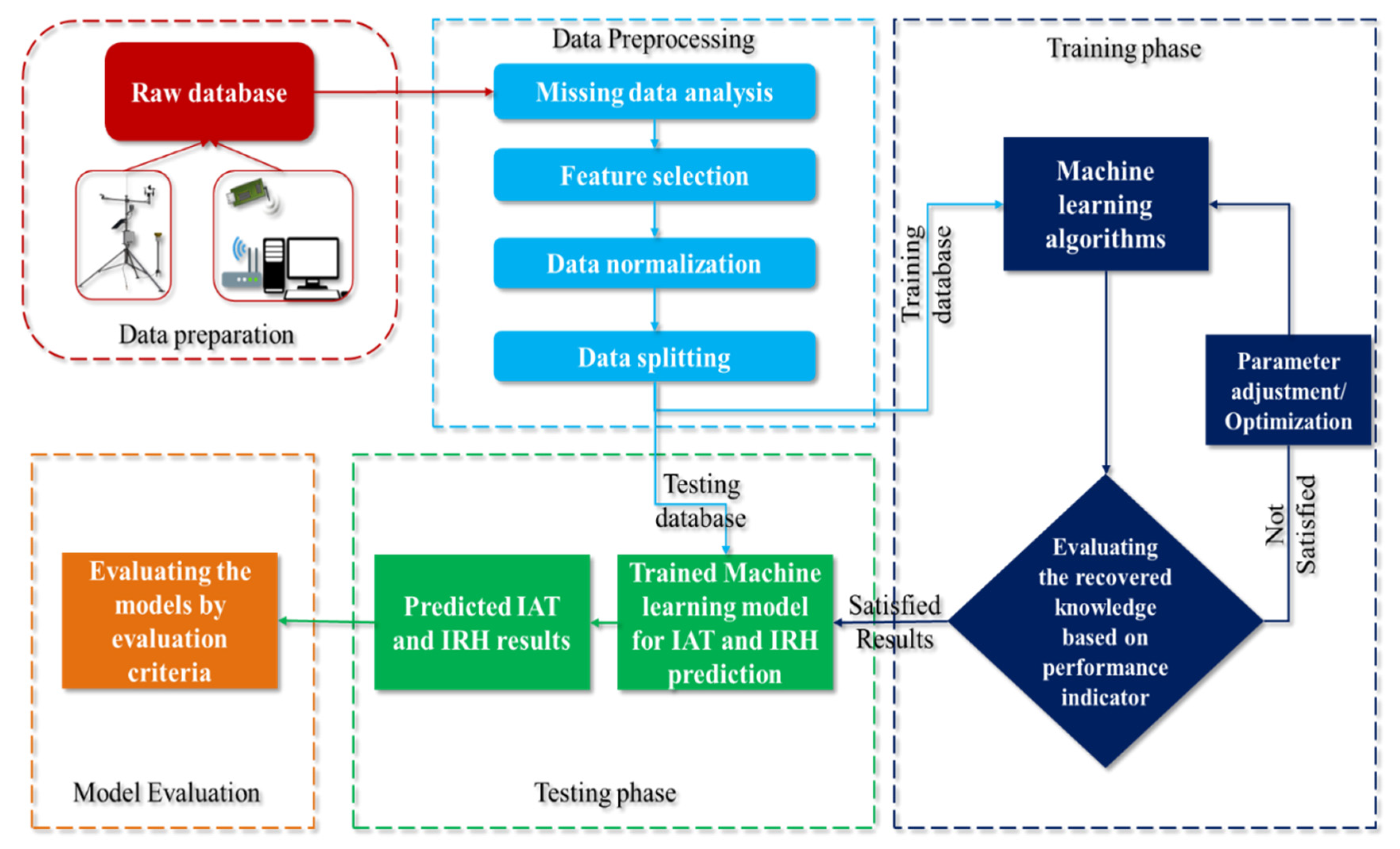
2.3. Approach
2.3.1. Multiple Linear Regression Model
2.3.2. Decision Tree Regression Model
2.3.3. Random Forest Regression Model
- Selecting random features,
- Bootstrap sampling,
- OOB error estimation to overcome stability issues, and
- Full depth decision tree growing.
2.3.4. Support Vector Regression Model
2.3.5. Multilayered Perceptron—Backpropagation Model
2.4. Choosing Input Datasets
2.5. Assumptions for Modeling
3. Results
3.1. Input Datasets
3.2. Model Performance
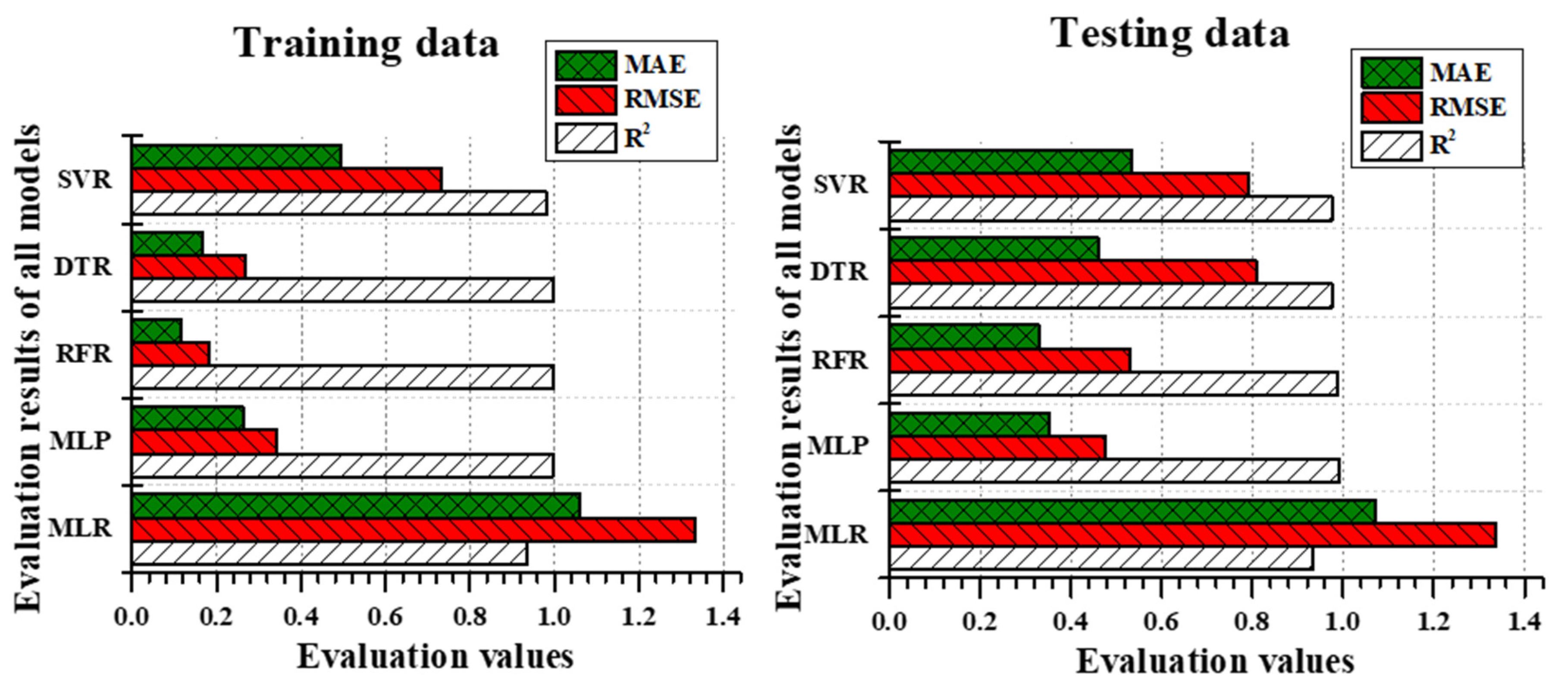
3.3. Model Comparison
4. Discussion
4.1. Model Selection
4.2. Model Accomplishment
5. Conclusions and Application
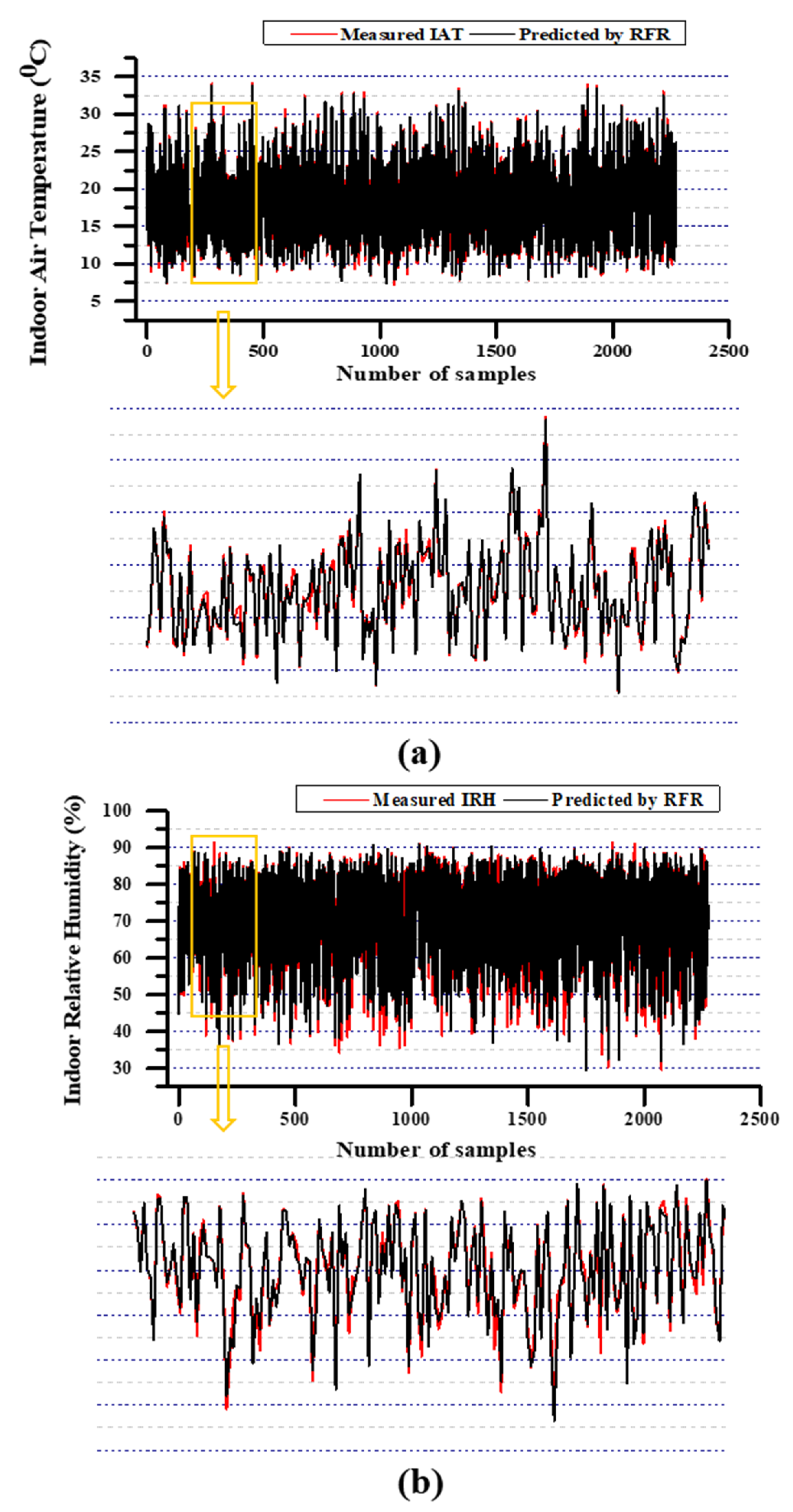
- The RFR models performed the most well among all the forecasting models used in this research most probably. RFR model has competent results in especially for IRH predictions compared with others. In addition, model-based control algorithms need to be developed for the real-time implementation of RFR based prediction integration in hardware.
- As seen in the results, the ML models used in this study have been more efficient than the statistical model. The statistical model was unable to make predictions when the data distribution is beyond the limit. Such models are limited to focus only on the linear relationship between variables. On the other hand, the ML models perform better with input variables that are complex and nonlinear due to the self-adaptive nature. ML models deem to be the optimal solver for the livestock indoor microclimatic control; since there are high fluctuations in the indoor environment of pig buildings and are very pervasive in general.
- The present study predicted IAT and IRH from accessible attributes without considering the animals’ biological factors. However, biological factors may affect the indoor climate still predictions of RFR have proven to simulate the parameters convincingly. Using accessible data rather than biological and non-accessible data can be better able to sustain human resources such as money, human needs, time, and technical resources such as computer usage, algorithm learning time, and model complexity.
- Selecting the right features from the given input data builds supportive conditions under which the expected results are available. Proving a greater number of attributes as input not only stifles the algorithm but also creates a confounding infrastructure to making the expected decisions. Witnessing the results of this study suggests that selecting the collect features is the most necessary process when modelling any indoor microclimate variables.
- The current study considered MLP, RFR, DTR, SVR, and MLR models to predict IAT and IRH. Recently deep learning (DL) and extreme learning machines (ELM) models are also enormously used to solve prediction problems. Such kind of models could be compared with the ML models in future studies. In addition, current literature used limited data due to the complication of collect indoor climate data for supervised learning. So in the future, big data for many cycles will be used to suggest an ultimate solution for controlling the indoor microclimate of swine buildings.
Author Contributions
Funding
Institutional Review Board Statement
Informed Consent Statement
Data Availability Statement
Acknowledgments
Conflicts of Interest
References
- Fróna, D.; János Szenderák, M.H.-R. The Challenge of Feeding the World. Sustainability 2019, 11, 5816. [Google Scholar] [CrossRef] [Green Version]
- Herrero, M.; Wirsenius, S.; Henderson, B.; Rigolot, C.; Thornton, P.; Havlík, P.; De Boer, I.; Gerber, P. Livestock and the Environment: What Have We Learned in the Past Decade? Annu. Rev. Environ. Resour. 2015, 40, 177–202. [Google Scholar] [CrossRef]
- Liberati, P.; Zappavigna, P. A dynamic computer model for optimization of the internal climate in swine housing design. Trans. ASABE 2007, 50, 2179–2188. [Google Scholar] [CrossRef]
- Machado, S.T.; Nääs, I.D.A.; Dos Reis, J.G.M.; Caldara, F.R.; Santos, R.C. Sows and piglets thermal comfort: A comparative study of the tiles used in the farrowing housing. Eng. Agric. 2016, 36, 996–1004. [Google Scholar] [CrossRef] [Green Version]
- Lee, S.J.; Oh, T.K.; Suk, K.I.M.; Min, W.G.; Gutierrez, W.M.; Chang, H.H.; Chikushi, J. Effects of environmental factors on death rate of pigs in Suth Korea. J. Fac. Agric. Kyushu Univ. 2012, 57, 155–160. [Google Scholar]
- Ottosen, M.; Mackenzie, S.G.; Wallace, M.; Kyriazakis, I. A method to estimate the environmental impacts from genetic change in pig production systems. Int. J. Life Cycle Assess. 2020, 25, 523–537. [Google Scholar] [CrossRef] [Green Version]
- Sejian, V.; Bhatta, R.; Gaughan, J.B.; Dunshea, F.R.; Lacetera, N. Review: Adaptation of animals to heat stress. Animal 2018, 12, S431–S444. [Google Scholar] [CrossRef] [Green Version]
- Schauberger, G.; Piringer, M.; Petz, E. Steady-state balance model to calculate the indoor climate of livestock buildings, demonstrated for finishing pigs. Int. J. Biometeorol. 2000, 43, 154–162. [Google Scholar] [CrossRef]
- Wu, Z.; Stoustrup, J.; Heiselberg, P. Parameter Estimation of Dynamic Multi-zone Models for Livestock Indoor Climate Control. In Proceedings of the 29th Air Infiltration and Ventilation Centre (AIVC) Conference, Kyoto, Japan, 14–16 October 2008; pp. 149–154. [Google Scholar]
- Molano-Jimenez, A.; Orjuela-Canon, A.D.; Acosta-Burbano, W. Temperature and Relative Humidity Prediction in Swine Livestock Buildings. In Proceedings of the 2018 IEEE Latin American Conference on Computational Intelligence (LA-CCI), Gudalajara, Mexico, 7–9 November 2018; pp. 2018–2021. [Google Scholar]
- Alizamir, M.; Kisi, O.; Ahmed, A.N.; Mert, C.; Fai, C.M.; Kim, S.; Kim, N.W.; El-Shafie, A. Advanced machine learning model for better prediction accuracy of soil temperature at different depths. PLoS ONE 2020, 15, e0231055. [Google Scholar] [CrossRef] [Green Version]
- Lee, W.; Ham, Y.; Ban, T.W.; Jo, O. Analysis of Growth Performance in Swine Based on Machine Learning. IEEE Access 2019, 7, 161716–161724. [Google Scholar] [CrossRef]
- Basak, J.K.; Okyere, F.G.; Arulmozhi, E.; Park, J.; Khan, F.; Kim, H.T. Artificial neural networks and multiple linear regression as potential methods for modelling body surface temperature of pig. J. Appl. Anim. Res. 2020, 48, 207–219. [Google Scholar] [CrossRef]
- Gorczyca, M.T.; Milan, H.F.M.; Maia, A.S.C.; Gebremedhin, K.G. Machine learning algorithms to predict core, skin, and hair-coat temperatures of piglets. Comput. Electron. Agric. 2018, 151, 286–294. [Google Scholar] [CrossRef] [Green Version]
- Ayaz, M.; Ammad-Uddin, M.; Sharif, Z.; Mansour, A.; Aggoune, E.H.M. Internet-of-Things (IoT)-based smart agriculture: Toward making the fields talk. IEEE Access 2019, 7, 129551–129583. [Google Scholar] [CrossRef]
- Besteiro, R.; Ortega, J.A.; Arango, T.; Rodriguez, M.R.; Fernandez, M.D.; Ortega, J.A. ARIMA modeling of animal zone temperature in weaned piglet buildings: Design of the model. Trans. ASABE 2017, 60, 2175–2183. [Google Scholar] [CrossRef]
- Ortega, J.A.; Losada, E.; Besteiro, R.; Arango, T.; Ginzo-Villamayor, M.J.; Velo, R.; Fernandez, M.D.; Rodriguez, M.R. Validation of an AutoRegressive Integrated Moving Average model for the prediction of animal zone temperature in a weaned piglet building. Biosyst. Eng. 2018, 174, 231–238. [Google Scholar] [CrossRef]
- Daskalov, P.I. Prediction of temperature and humidity in a naturally ventilated pig building. J. Agric. Eng. Res. 1997, 68, 329–339. [Google Scholar] [CrossRef]
- Neethirajan, S. Transforming the adaptation physiology of farm animals through sensors. Animals 2020, 10, 1512. [Google Scholar] [CrossRef]
- Liu, S.; Wang, X.; Liu, M.; Zhu, J. Towards better analysis of machine learning models: A visual analytics perspective. Vis. Inform. 2017, 1, 48–56. [Google Scholar] [CrossRef]
- Czarnecki, W.M.; Podolak, I.T. Machine learning with known input data uncertainty measure. Lect. Notes Comput. Sci. Incl. Subser. Lect. Notes Artif. Intell. Lect. Notes Bioinform. 2013, 8104, 379–388. [Google Scholar] [CrossRef]
- Schmidt, J.; Marques, M.R.G.; Botti, S.; Marques, M.A.L. Recent advances and applications of machine learning in solid-state materials science. npj Comput. Mater. 2019, 5. [Google Scholar] [CrossRef]
- Arulmozhi, E.; Basak, J.K.; Park, J.; Okyere, F.G.; Khan, F.; Lee, Y.; Lee, J.; Lee, D.; Kim, H.T. Impacts of nipple drinker position on water intake, water wastage and drinking duration of pigs. Turk. J. Vet. Anim. Sci. 2020, 44, 562–572. [Google Scholar] [CrossRef]
- Ravn, P. Characteristics of Floors for Pig Pens: Friction, shock absorption, ammonia emission and heat conduction. Agric. Eng. Int. CIGR J. 2008, X, 1–16. [Google Scholar]
- Zhao, T.; Xue, H. Regression analysis and indoor air temperature model of greenhouse in northern dry and cold regions. IFIP Adv. Inf. Commun. Technol. 2011, 345, 252–258. [Google Scholar] [CrossRef] [Green Version]
- Taki, M.; Ajabshirchi, Y.; Ranjbar, S.F.; Matloobi, M. Application of neural networks and multiple regression models in greenhouse climate estimation. Agric. Eng. Int. CIGR J. 2016, 18, 29–43. [Google Scholar]
- Elanchezhian, A.; Basak, J.K.; Park, J.; Khan, F.; Okyere, F.G.; Lee, Y.; Bhujel, A.; Lee, D.; Sihalath, T.; Kim, H.T. Evaluating different models used for predicting the indoor microclimatic parameters of a greenhouse. Appl. Ecol. Environ. Res. 2020, 18, 2141–2161. [Google Scholar] [CrossRef]
- Basak, J.K.; Arulmozhi, E.; Khan, F.; Okyere, F.G.; Park, J.; Kim, H.T. Modeling of ambient environment and thermal status relationship of pig’s body in a pig barn. Indian J. Anim. Res. 2020, 54, 1049–1054. [Google Scholar] [CrossRef]
- Wen, L.; Ling, J.; Saintilan, N.; Rogers, K. An investigation of the hydrological requirements of River Red Gum (Eucalyptus camaldulensis) Forest, using Classification and Regression Tree modelling. Ecohydrology 2009, 2, 143–155. [Google Scholar] [CrossRef]
- Aguilera, J.J.; Andersen, R.K.; Toftum, J. Prediction of indoor air temperature using weather data and simple building descriptors. Int. J. Environ. Res. Public Health 2019, 16, 4349. [Google Scholar] [CrossRef] [Green Version]
- Walker, S.; Khan, W.; Katic, K.; Maassen, W.; Zeiler, W. Accuracy of different machine learning algorithms and added-value of predicting aggregated-level energy performance of commercial buildings. Energy Build. 2020, 209, 109705. [Google Scholar] [CrossRef]
- Vassallo, D.; Krishnamurthy, R.; Sherman, T.; Fernando, H.J. Analysis of Random Forest Modeling Strategies for Multi-Step Wind Speed Forecasting. Energies 2020, 5488. [Google Scholar] [CrossRef]
- Drucker, H.; Surges, C.J.C.; Kaufman, L.; Smola, A.; Vapnik, V. Support vector regression machines. Adv. Neural Inf. Process. Syst. 1997, 1, 155–161. [Google Scholar]
- Wu, J.; Liu, H.; Wei, G.; Song, T.; Zhang, C.; Zhou, H. Flash flood forecasting using support vector regression model in a small mountainous catchment. Water 2019, 11, 1327. [Google Scholar] [CrossRef] [Green Version]
- Hasan, N.; Nath, N.C.; Rasel, R.I. A support vector regression model for forecasting rainfall. 2nd Int. Conf. Electr. Inf. Commun. Technol. EICT 2015 2016, 554–559. [Google Scholar] [CrossRef]
- Kumar, S.; Chong, I. Correlation analysis to identify the effective data in machine learning: Prediction of depressive disorder and emotion states. Int. J. Environ. Res. Public Health 2018, 15, 2907. [Google Scholar] [CrossRef] [Green Version]
- Medar, R.; Rajpurohit, V.S.; Rashmi, B. Impact of training and testing Data splits on accuracy of time series forecasting in Machine Learning. In Proceedings of the International Conference on Computing, Communication, Control and Automation (ICCUBEA), Pune, India, 17–18 August 2017; pp. 1–6. [Google Scholar]
- Lakshminarayan, K.; Harp, S.; Goldman, R.; Samad, T. Imputation of Missing Data Using Machine Learning Techniques. In Proceedings of the Second International Conference on Knowledge Discovery and Data Miming (KDD-96); AAAI Press: Portland, OR, USA, 1996; pp. 140–145. [Google Scholar]
- Sola, J.; Sevilla, J. Importance of input data normalization for the application of neural networks to complex industrial problems. IEEE Trans. Nucl. Sci. 1997, 44, 1464–1468. [Google Scholar] [CrossRef]
- Jayalakshmi, T.; Santhakumaran, A. Statistical Normalization and Back Propagationfor Classification. Int. J. Comput. Theory Eng. 2011, 3, 89–93. [Google Scholar] [CrossRef]
- Munkhdalai, L.; Munkhdalai, T.; Park, K.H.; Lee, H.G.; Li, M.; Ryu, K.H. Mixture of Activation Functions with Extended Min-Max Normalization for Forex Market Prediction. IEEE Access 2019, 7, 183680–183691. [Google Scholar] [CrossRef]
- Mohan, P.; Patil, K.K. Deep learning based weighted SOM to forecast weather and crop prediction for agriculture application. Int. J. Intell. Eng. Syst. 2018, 11, 167–176. [Google Scholar] [CrossRef]
- Singh, S.A.; Majumder, S. Short unsegmented PCG classification based on ensemble classifier. Turk. J. Electr. Eng. Comput. Sci. 2020, 28, 875–889. [Google Scholar] [CrossRef]
- Kontokosta, C.E.; Tull, C. A data-driven predictive model of city-scale energy use in buildings. Appl. Energy 2017, 197, 303–317. [Google Scholar] [CrossRef] [Green Version]
- Seo, I.; Lee, I.; Moon, O.; Hong, S.; Hwang, H.; Bitog, J.P.; Kwon, K.; Ye, Z.; Lee, J. Modelling of internal environmental conditions in a full-scale commercial pig house containing animals. Biosyst. Eng. 2012, 111, 91–106. [Google Scholar] [CrossRef]
- Tuomisto, H.L.; Scheelbeek, P.F.D.; Chalabi, Z.; Green, R.; Smith, R.D.; Haines, A.; Dangour, A.D. Effects of environmental change on population nutrition and health: A comprehensive framework with a focus on fruits and vegetables. Wellcome Open Res. 2017, 2, 21. [Google Scholar] [CrossRef] [PubMed] [Green Version]


| S. No | Attribute | Elements/Predictors (Unit) | Mean ± SD | SE | Min | Max |
|---|---|---|---|---|---|---|
| 1 | WD | Wind direction (°(Azimuth)) | 205.0 ± 67.43 | 0.632 | 29.4 | 337.2 |
| 2 | WS | Wind speed (m/s) | 0.644 ± 0.379 | 0.003 | 0.11 | 4.55 |
| 3 | OAT | Outdoor air temperature (°C) | 12.858 ± 6.729 | 0.063 | −2.7 | 31 |
| 4 | ORH | Outdoor relative humidity (%) | 72.746 ± 22.082 | 0.207 | 13.78 | 96.9 |
| 5 | AP | Outdoor air pressure (Pa) | 1013.916 ± 5.495 | 0.051 | 976 | 1024 |
| 6 | RFA | Rain fall amount (inch) | 0.0057 ± 0.059 | 0.0005 | 0 | 1.71 |
| 7 | SLR | Solar irradiance (Wm-2) | 124.722 ± 199.280 | 1.869 | 0 | 889 |
| 8 | SMC | Soil moisture content (%) | 17.325 ± 1.722 | 0.016 | 13.88 | 29.62 |
| 9 | ST | Outdoor soil temperature (°C) | 13.851 ± 6.229 | 0.058 | 2.622 | 30.26 |
| 10 | CNR | Net radiation (Wm-2) | 31.037 ± 149.867 | 1.406 | −161.8 | 645.1 |
| S. No | Attribute | Elements/Response (Unit) | Mean ± SD | SE | Min | Max |
| 1 | IAT | Indoor air temperature (°C) | 18.294 ± 5.22 | 0.048 | 6.7 | 34.2 |
| 2 | IRH | Indoor relative humidity (%) | 70.122 ± 12.179 | 0.114 | 25.5 | 92.3 |
| Model | Datasets | Description | Response |
|---|---|---|---|
| S1 | WD, WS, OAT, ORH, AP, RFA, SLR, SW, ST, CNR | All Collected parameters from weather station | IAT |
| S2 | WD, WS, OAT, ORH, AP, RFA, SLR, SW, ST, CNR, IRH | All Collected parameters from weather station including indoor parameters | IAT |
| S3 | OAT, ORH, ST, SLR, IRH | Selected feature by using correlation matrix (Including positive and negative relationship by using Spearman rank correlation coefficient approach) | IAT |
| S1 | WD, WS, OAT, ORH, AP, RFA, SLR, SW, ST, CNR | All Collected parameters from weather station | IRH |
| S2 | WD, WS, OAT, ORH, AP, RFA, SLR, SW, ST, CNR, IAT | All Collected parameters from weather station including indoor parameters | IRH |
| S3 | ORH, SLR, CNR IAT | Selected feature by using correlation matrix (Including positive and negative relationship by using Spearman rank correlation coefficient approach) | IRH |
| Algorithms | Hyper Parameters | Distribution (Range) |
|---|---|---|
| Multiple linear regression (MLR) | - | - |
| Multilayered perceptron (MLP) | Number of Hidden layers | *Ud (1, 4) |
| Number of Hidden neurons | Ud (1, 250) | |
| Learning rate | Adaptive | |
| Solver | Adam | |
| Activation function | Relu | |
| Decision tree regression (DTR) | Maximum depth | Ud (1, 100) |
| Minimum sample split | Ud (2, 10) | |
| Minimum sample leaf | Ud (1, 4) | |
| Support vector regression (SVR) | Kernel | Radial-basis function |
| C | Ud (1, 100) | |
| Gamma | 1 | |
| Epsilon | 0.1 | |
| Random forest regression (RFR) | Number of trees | Ud (10, 250) |
| Minimum number of observations in a leaf | Ud (1, 30) | |
| Number of variables used in each split | Ud (1, 4) | |
| Maximum tree depth | Ud (1, 100) |
| S1 | ||||||
|---|---|---|---|---|---|---|
| Models | Training | Validation | ||||
| MAE * | RMSE * | R2 * | MAE | RMSE | R2 | |
| MLR | 1.2022 | 1.5202 | 0.9159 | 1.2254 | 1.558 | 0.9076 |
| MLP | 0.2832 | 0.3808 | 0.9947 | 0.3719 | 0.5301 | 0.9893 |
| RFR | 0.1271 | 0.2088 | 0.9984 | 0.3574 | 0.5807 | 0.9871 |
| DTR | 0.1939 | 0.3351 | 0.9959 | 0.4979 | 0.899 | 0.9692 |
| SVR | 0.6731 | 0.9865 | 0.9645 | 0.7302 | 1.0878 | 0.9549 |
| S2 | ||||||
| Models | Training | Validation | ||||
| MAE | RMSE | R2 | MAE | RMSE | R2 | |
| MLR | 1.0772 | 1.3557 | 0.9331 | 1.087 | 1.3551 | 0.9301 |
| MLP | 0.3968 | 0.54 | 0.9893 | 0.4459 | 0.621 | 0.9853 |
| RFR | 0.126 | 0.2013 | 0.9985 | 0.3641 | 0.5903 | 0.9867 |
| DTR | 0.1933 | 0.3194 | 0.9962 | 0.5003 | 0.8539 | 0.9722 |
| SVR | 0.5846 | 0.8204 | 0.9755 | 0.6097 | 0.8613 | 0.9717 |
| S3 | ||||||
| Models | Training | Validation | ||||
| MAE | RMSE | R2 | MAE | RMSE | R2 | |
| MLR | 1.061 | 1.332 | 0.9354 | 1.0721 | 1.3352 | 0.9321 |
| MLP | 0.2628 | 0.3434 | 0.9957 | 0.3535 | 0.4763 | 0.9913 |
| RFR | 0.1165 | 0.1833 | 0.9987 | 0.3282 | 0.5283 | 0.9893 |
| DTR | 0.1648 | 0.2683 | 0.9973 | 0.4595 | 0.8081 | 0.9751 |
| SVR | 0.4936 | 0.7333 | 0.9804 | 0.5331 | 0.7911 | 0.9761 |
| S1 | ||||||
|---|---|---|---|---|---|---|
| Models | Training | Validation | ||||
| MAE | RMSE | R2 | MAE | RMSE | R2 | |
| MLR | 4.9058 | 6.2697 | 0.7361 | 5.1502 | 6.589 | 0.7019 |
| MLP | 3.3399 | 4.503 | 0.8638 | 3.5312 | 4.7917 | 0.8423 |
| RFR | 0.5931 | 0.9607 | 0.9938 | 1.5963 | 2.6222 | 0.9527 |
| DTR | 0.8047 | 1.3866 | 0.987 | 2.0807 | 3.5936 | 0.9113 |
| SVR | 0.2385 | 0.6668 | 0.997 | 2.4453 | 4.028 | 0.8886 |
| S2 | ||||||
| Models | Training | Validation | ||||
| MAE | RMSE | R2 | MAE | RMSE | R2 | |
| MLR | 4.4651 | 5.8377 | 0.7712 | 4.6572 | 6.0534 | 0.7484 |
| MLP | 3.238 | 4.4669 | 0.866 | 3.4088 | 4.7072 | 0.8478 |
| RFR | 0.7206 | 1.1475 | 0.9911 | 1.9392 | 3.0872 | 0.9345 |
| DTR | 1.6783 | 2.635 | 0.9533 | 2.6972 | 4.3607 | 0.8694 |
| SVR | 0.8696 | 1.1269 | 0.9914 | 2.1301 | 3.4244 | 0.9194 |
| S3 | ||||||
| Models | Training | Validation | ||||
| MAE | RMSE | R2 | MAE | RMSE | R2 | |
| MLR | 4.1603 | 5.4935 | 0.7974 | 4.3323 | 5.653 | 0.78058 |
| MLP | 2.4782 | 3.5452 | 0.9156 | 2.5856 | 3.7046 | 0.9057 |
| RFR | 0.5494 | 0.8847 | 0.9947 | 1.4708 | 2.429 | 0.9594 |
| DTR | 0.7985 | 1.3353 | 0.988 | 2.0876 | 3.6876 | 0.9066 |
| SVR | 0.1671 | 0.3896 | 0.9989 | 2.2302 | 3.8161 | 0.9 |
Publisher’s Note: MDPI stays neutral with regard to jurisdictional claims in published maps and institutional affiliations. |
© 2021 by the authors. Licensee MDPI, Basel, Switzerland. This article is an open access article distributed under the terms and conditions of the Creative Commons Attribution (CC BY) license (http://creativecommons.org/licenses/by/4.0/).
Share and Cite
Arulmozhi, E.; Basak, J.K.; Sihalath, T.; Park, J.; Kim, H.T.; Moon, B.E. Machine Learning-Based Microclimate Model for Indoor Air Temperature and Relative Humidity Prediction in a Swine Building. Animals 2021, 11, 222. https://doi.org/10.3390/ani11010222
Arulmozhi E, Basak JK, Sihalath T, Park J, Kim HT, Moon BE. Machine Learning-Based Microclimate Model for Indoor Air Temperature and Relative Humidity Prediction in a Swine Building. Animals. 2021; 11(1):222. https://doi.org/10.3390/ani11010222
Chicago/Turabian StyleArulmozhi, Elanchezhian, Jayanta Kumar Basak, Thavisack Sihalath, Jaesung Park, Hyeon Tae Kim, and Byeong Eun Moon. 2021. "Machine Learning-Based Microclimate Model for Indoor Air Temperature and Relative Humidity Prediction in a Swine Building" Animals 11, no. 1: 222. https://doi.org/10.3390/ani11010222