Linearizing Control of a Distributed Actuation Magnetic Bearing for Thin-Walled Rotor Systems

Abstract

This paper describes an exact linearizing control approach for a distributed actuation magnetic bearing (DAMB) supporting a thin-walled rotor. The radial DAMB design incorporates a circular array of compact electromagnetic actuators with multi-coil winding scheme optimized for supporting thin-walled rotors. A distinguishing feature is that both the x and y components of the radial bearing force are coupled with all four of the supplied coil currents and so a closed form solution for the linearizing equations cannot be obtained. To overcome this issue, a gradient-based root-finding algorithm is proposed to solve the linearizing equations numerically in real-time. The proposed method can be applied with any chosen constraints on current values to achieve low RMS values while avoiding zero-current operating points. The approach is implemented and tested experimentally on a rotor system comprising two radial DAMBs and a uniform cylindrical shell rotor. The results show that the method achieves more accurate reproduction of demanded bearing forces, thereby simplifying the rotor suspension control design and providing improved stability and vibration control performance compared with implementations based on operating point linearization.

1. Introduction

Active magnetic bearings (AMBs) incorporate electromagnetic actuators to achieve contact-free suspension of rotating shafts. They have important advantages over conventional bearings and can enable high speed, low vibration and low maintenance operation of rotating machines. A typical radial AMB is formed from pairs of electromagnets that apply opposing attractive forces to a rotor shaft, as shown in Figure 1. Feedback control of actuator coil currents based on measured rotor displacements is used to stabilize the rotor positioning within the bearing and prevent excessive vibration [1,2]. Although AMBs have been widely applied with solid-shaft rotors, there has been recent research interest in the design and application of AMBs with hollow and ring-like rotors [3,4,5,6]. In the case of thin-walled rotors, a larger number of smaller actuators may be incorporated within the bearing to support the rotor around its periphery [5]. However, this results in a more complex relation between the forces acting on the rotor and the currents within the actuator coils, which brings challenges in achieving exact or approximate linearization of the bearing force behavior within a control algorithm. Before describing the problem in detail, a brief review of the state of the art for conventional radial AMBs is provided.

A radial magnetic bearing is usually designed to operate in the linear B-H region [7,8]. Considering a single actuator within the bearing having two pole faces of area $A_p$ and a uniform gap of size s from the rotor, the attractive force (neglecting curvature) is given by [1]

$$F={\mathsf{\mu }}_0{A}_p{\left(\frac{Ni}{l_{iron}/{\mathsf{\mu }}_r+2s}\right)}^2$$

(1)

where N is the number of coil turns, i is the coil current, ${\mathsf{\mu }}_0$ is the permeability of free space, ${\mathsf{\mu }}_r$ is the relative permeability of the core material and $l_{iron}$ is the mean flux path length through the actuator core and rotor.

Although the actuator forces are described by nonlinear equations, for feedback control, the relationship between the magnetic force and change in current can be approximated by a linear relation when operating with sufficiently high bias currents [9]. This is usually achieved with a differential driving scheme, where time-varying control currents $i_x^c$ and $i_y^c$ are added and subtracted to a constant bias current $i_0$ for actuators on opposite sides of the rotor, as illustrated in Figure 1. From (1), the resultant force (in the x-axis direction) will be

$$F_x\left(t\right)={\mathsf{\mu }}_0{A}_{p}N\left({\left(\frac{i_0+i_x^c\left(t\right)}{l_0-2x\left(t\right)}\right)}^2-{\left(\frac{i_0-i_x^c\left(t\right)}{l_0+2x\left(t\right)}\right)}^2\right)$$

(2)

For this equation, x is the displacement of the rotor from the bearing center and the effective flux path length is $l_0=l_{iron}/{\mathsf{\mu }}_r+2s_0$ where $s_0$ is the gap size when $x=0$.

Using higher values for the bias current can widen the range of linear behavior but has disadvantages of increased coil heating and energy losses. Therefore, a number of researchers have investigated radial AMB operation with low or zero bias currents. Using permanent magnets (PMs) to generate bias flux is one possible approach. This was considered by Zheng et al. to reduce power consumption in a control moment gyro (CMG) system [10]. Design considerations in the use of PM biasing for radial/axial and combination AMBs are described in Reference [11]. Meeker and Maslen considered the generalized bias linearization problem for a radial magnetic bearing in Reference [12], where a linear transformation of coil current values, computed offline, is used to generate a linear dependency on bearing forces for a given rotor position.

As using low bias current values accentuates the nonlinear force characteristics of the bearing, nonlinear control methods become more appropriate [13,14]. To improve load capacity, Gerami et al. presented a nonlinear magnetization model and control of a radial AMB with high-level magnetization [15]. Chen and Song implemented a dynamics bias current control strategy to stabilize an AMB system and minimize energy consumption [16].

For feedback linearization, an analytical inverse model of the bearing is usually employed within the control algorithm so that the actual bearing force exactly matches the demanded value from the feedback control law [17,18]. This control scheme is advantageous as it allows the control algorithm to be designed based on the linear dynamics of the free rotor, as shown in Figure 2. To overcome the difficulties in obtaining an accurate analytical model of the bearing forces, feedback linearization using a look-up table approach was considered in Reference [19] for an AMB operating in current control mode. Feedback linearization and control system design for a 1-d.o.f. AMB actuator was considered by Mystkowski et al. [20], where two approaches based on voltage switching and flux control were formulated and evaluated in simulation. Feedback linearization for a single voltage-controlled magnetic bearing actuator was considered in Reference [21].

This paper considers the feedback linearization problem for a novel design of radial magnetic bearing with distributed actuation topology. The distributed actuation magnetic bearing (DAMB) incorporates a multiplicity of small electromagnetic actuators in an arrangement that is suited to supporting hollow lightweight and thin-walled rotors [5]. A distinguishing feature is that both the x and y force components couple with all four of the supplied coil currents, and hence the linearization problem cannot be separated into x and y axis subsystems. Moreover, a closed form solution of the linearizing equations cannot be obtained. Due to these features, feedback linearization methods such as those in References [17,18,19,20,21] are not applicable and an approach based on numerical solution of the linearizing equations in real-time is therefore proposed. Section 2 provides details of the bearing design and theoretical model. The exact linearization control method is presented in Section 3. Simulation and experimental results are described in Section 4 to validate the proposed approach. The final section provides conclusions.

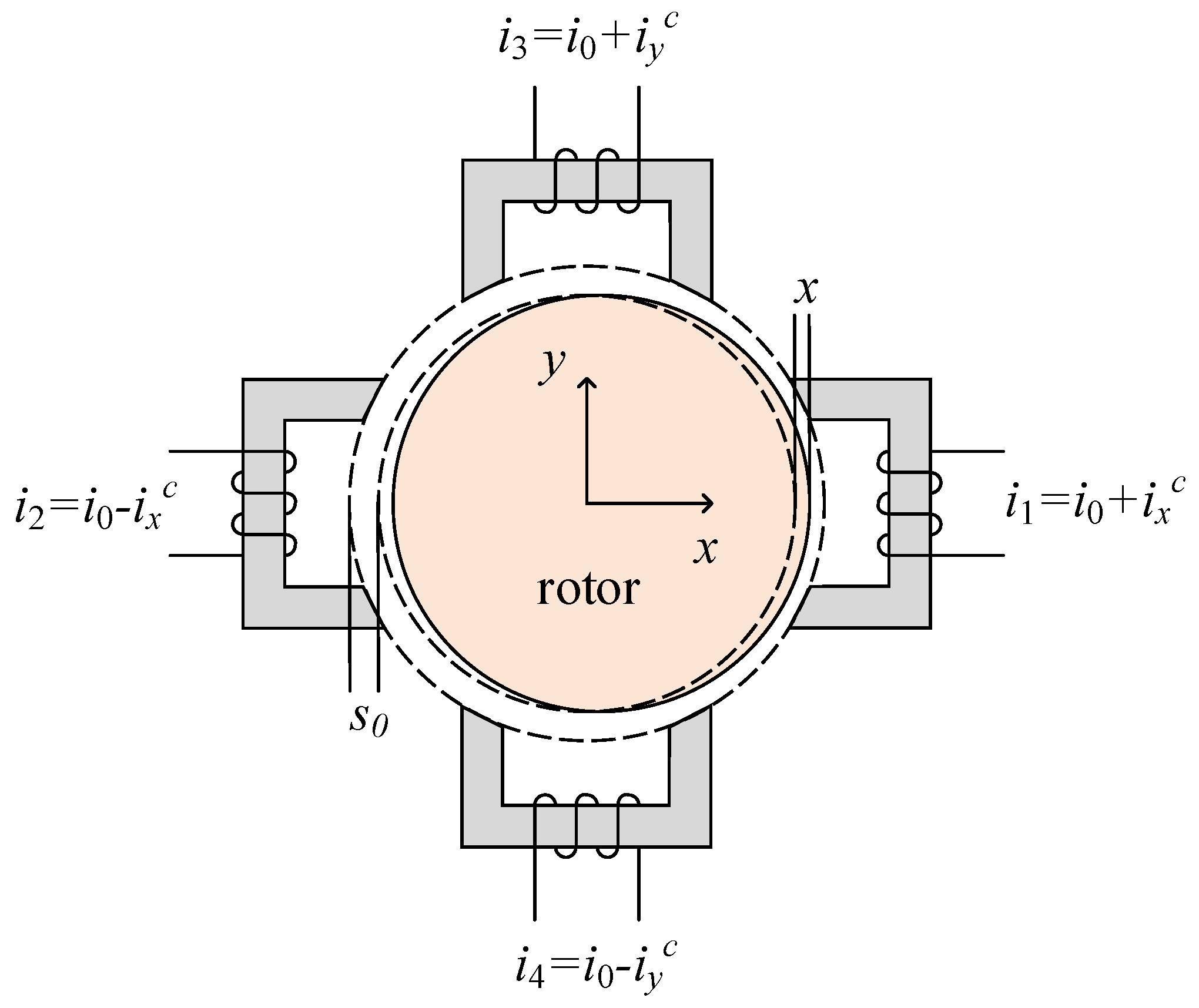
2. DAMB Design and Force Model

A lightweight thin-walled rotor structure may be considered that is a shell of revolution with large diameter compared with the wall thickness. Compared with a solid or thick-walled rotor, there is a relatively small cross sectional area for the bearing magnetic flux to pass through. Therefore, a conventional radial AMB design is not appropriate to support the structure. A radial bearing design based on the DAMB concept is shown in Figure 3. It comprises a circular array of relatively small electromagnetic actuators fixed to the bearing stator. The actuators have a U-shaped core with magnetic flux path aligned axially with the rotor, similar to a conventional homopolar magnetic bearing. Note that lamination of the rotor wall is not possible and so a homopolar arrangement is appropriate to reduce eddy current losses. The sizing of the actuator is chosen to match the rotor wall thickness such that the onset of flux saturation within the actuator core, and within the rotor material, would occur simultaneously. This condition is required to maximize bearing capacity and leads to a larger number of smaller actuators compared with the conventional AMB, where typically only four stator pole-pairs are employed (see Figure 1).

A further special feature of the design is that each actuator has two independently powered coils. Suppose the coils on the $j\mathrm{th}$ actuator have number of turns $N_{1,j}$ and $N_{2,j}$, and have regulated current $i_{1,j}$ and $i_{2,j}$, respectively. According to (1), the $j\mathrm{th}$ actuator at angular position ${\theta }_j$ applies an attractive radial force to the rotor given by

$$F_j={\mathsf{\mu }}_0{A}_p\frac{{\left(N_{1,j}{i}_{1,j}+N_{2,j}{i}_{2,j}\right)}^2}{{\left(l_0-2u_j\right)}^2}$$

(3)

where $u_j=xcos{\theta }_j+ysin{\theta }_j$ is the radial displacement of the rotor at the $j\mathrm{th}$ actuator with $(x,y)$ denoting the rotor lateral displacements within the bearing.

The load capacity of the magnetic bearing depends on the total pole-face area and the magnetic flux saturation limit (which is material dependent). Therefore, the load capacity for the DAMB will be similar to a conventional AMB if the total pole face area is similar. The main issue from downsizing of the actuators is that the same current-turns ($Ni$) must be realized within a smaller coil volume and this results in greater heating and more stringent requirements for heat dissipation. Achieving low mean current values without introducing significant nonlinear dynamics for the controlled system is therefore strongly motivated.

To produce a resultant force in any radial direction, the actuator coils are connected in series with four current control drives that supply currents $i_x^{+}$, $i_x^{-}$, $i_y^{+}$ and $i_y^{-}$ based on which quadrant the actuator is located in [5]:

$$\begin{array}{ccc}{i}_{1,j}=i_x^{+}\mathrm{and}{i}_{2,j}=i_y^{+}& \mathrm{for}& 0\le {\theta }_j\le \pi /2,\\ i_{1,j}=i_x^{-}\mathrm{and}{i}_{2,j}=i_y^{+}& \mathrm{for}& \pi /2\le {\theta }_j\le \pi \\ i_{1,j}=i_x^{-}\mathrm{and}{i}_{2,j}=i_y^{-}& \mathrm{for}& \pi \le {\theta }_j\le 3\pi /2\\ i_{1,j}=i_x^{+}\mathrm{and}{i}_{2,j}=i_y^{-}& \mathrm{for}& 3\pi /2\le {\theta }_j\le 2\pi \end{array}$$

(4)

From (3), the x and y components of the resultant force acting on the rotor can be expressed

$$F_x=\sum F_{j}cos{\theta }_j=a_1{i}_x^{+}{i}_y^{+}+a_2{i}_x^{+}{i}_y^{-}+a_3{i}_x^{-}{i}_y^{+}+a_4{i}_x^{-}{i}_y^{-}+a_5{i}_x^{{+}^2}+a_6{i}_x^{{-}^2}+a_7{i}_y^{{+}^2}+a_8{i}_y^{{-}^2}$$

(5)

$$F_y=\sum F_{j}sin{\theta }_j=b_1{i}_x^{+}{i}_y^{+}+b_2{i}_x^{+}{i}_y^{-}+b_3{i}_x^{-}{i}_y^{+}+b_4{i}_x^{-}{i}_y^{-}+b_5{i}_x^{{+}^2}+b_6{i}_x^{{-}^2}+b_7{i}_y^{{+}^2}+b_8{i}_y^{{-}^2}$$

(6)

where the coefficient values vary with rotor position according to the formulae given in

Table 1. Position-dependent coefficients for the bearing force Equations (5) and (6).

Coefficient	Formula *	Coefficient	Formula *
$a_1,a_2,a_3,a_4$	${\mathsf{\mu }}_0{A}_p\sum \frac{2N_{1,j}{N}_{2,j}}{{\left(l_0-2u_j\right)}^2}cos{\theta }_j$	$b_1,b_2,b_3,b_4$	${\mathsf{\mu }}_0{A}_p\sum \frac{2N_{1,j}{N}_{2,j}}{{\left(l_0-2u_j\right)}^2}sin{\theta }_j$
$a_5,a_6$	${\mathsf{\mu }}_0{A}_p\sum \frac{N_{1,j}^2}{{\left(l_0-2u_j\right)}^2}cos{\theta }_j$	$b_5,b_6$	${\mathsf{\mu }}_0{A}_p\sum \frac{N_{1,j}^2}{{\left(l_0-2u_j\right)}^2}sin{\theta }_j$
$a_7,a_8$	${\mathsf{\mu }}_0{A}_p\sum \frac{N_{2,j}^2}{{\left(l_0-2u_j\right)}^2}cos{\theta }_j$	$b_7,b_8$	${\mathsf{\mu }}_0{A}_p\sum \frac{N_{2,j}^2}{{\left(l_0-2u_j\right)}^2}sin{\theta }_j$

* The summation here is over j falling within the appropriate quadrant according to Equation (4).

. For given force values, (5) and (6) are coupled quadratic equations in the four current variables. To obtain a unique solution, additional constraints must be introduced for the coil currents. However, even with linear constraints, a closed form solution may not exist. To deal with a generalized case, a numerical method to find solutions in real-time is introduced in the following section.

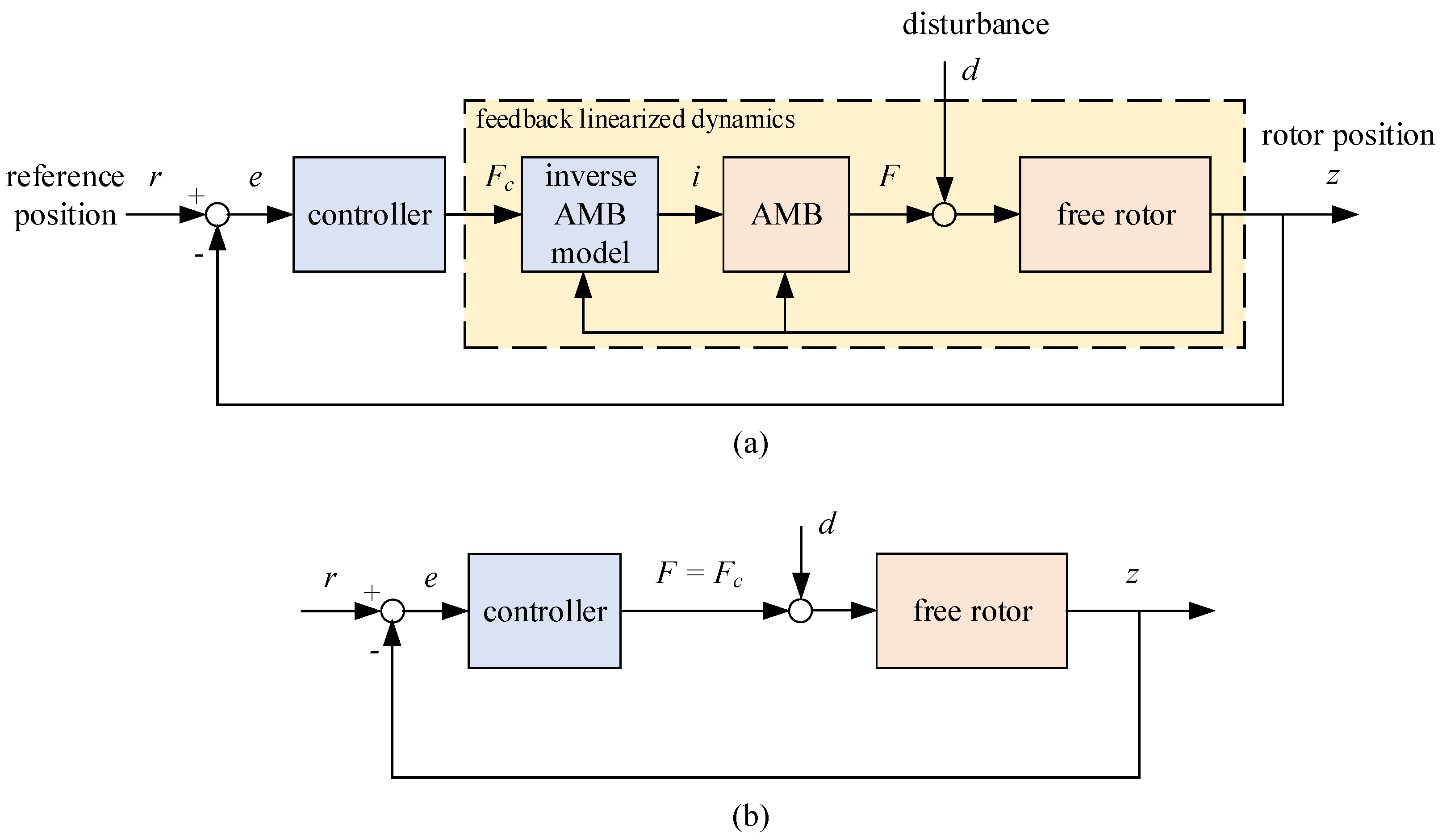
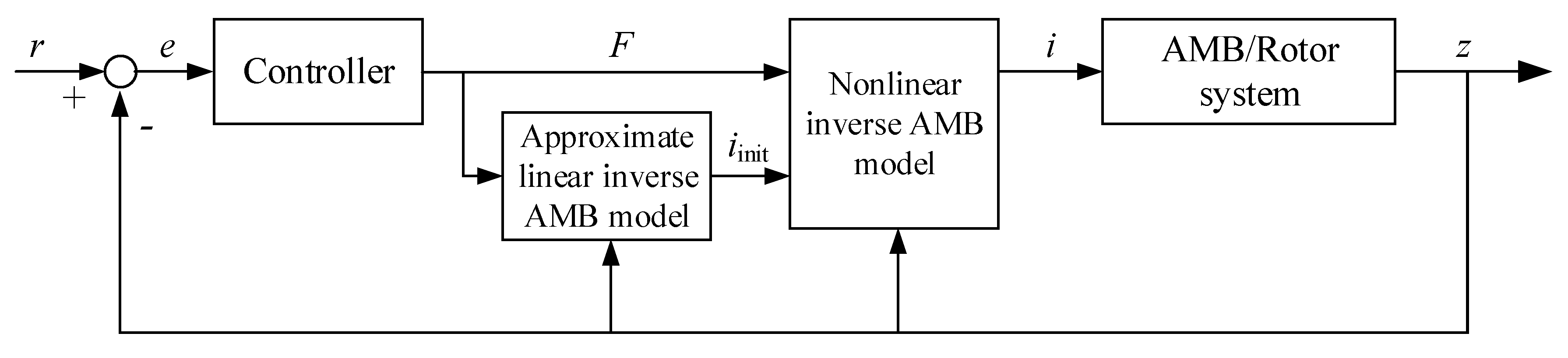
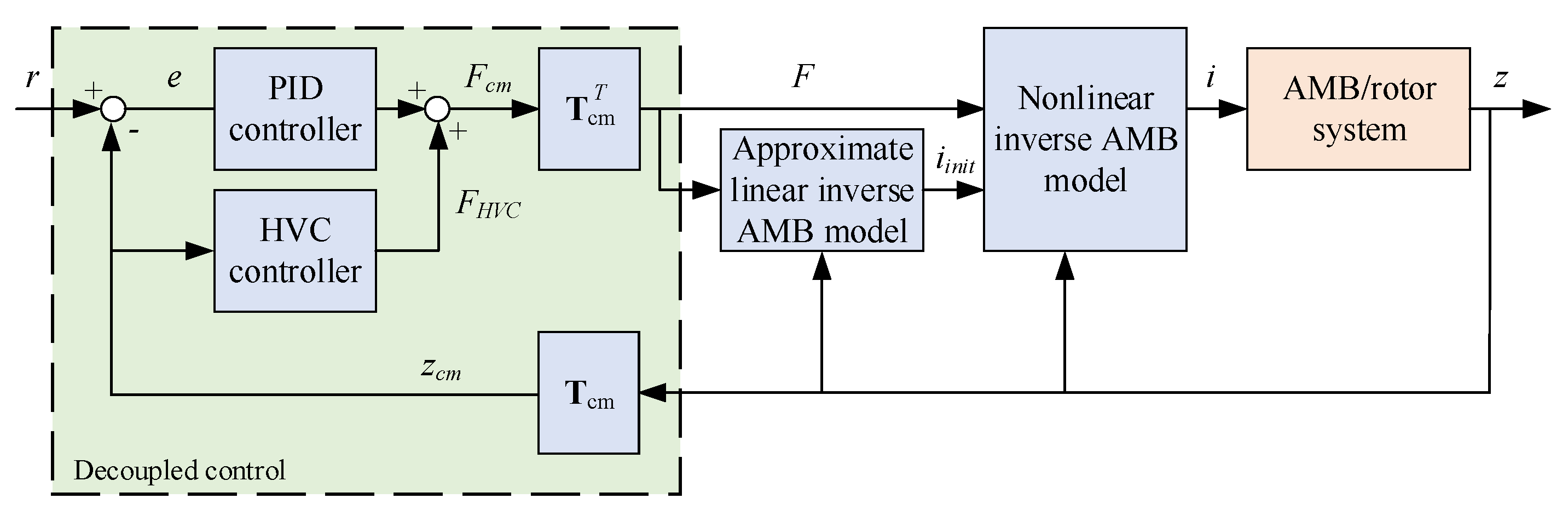
3. Exact Linearizing Control

If a conventional differential driving mode is adopted with constant bias current $i_0$, then $i_{x,y}^{+}=i_0+i_{x,y}^c$, $i_{x,y}^{-}=i_0-i_{x,y}^c$. Substituting these in (5) and (6) yields a pair of coupled quadratic equations in $i_x^c$ and $i_y^c$. In this case, after some algebraic manipulation, the solution can be found from a root-calculation problem for a fourth order polynomial. Although this solution can be obtained analytically, for practical implementation it is preferable to consider a more general situation where the control currents have other types of constraints imposed, including those that involve saturation limits. Therefore, an alternative approach considered in this paper is to use a gradient-based root-finding algorithm within the feedback control computations. Moreover, the proposed approach is shown to be sufficiently reliable and efficient for real-time control.

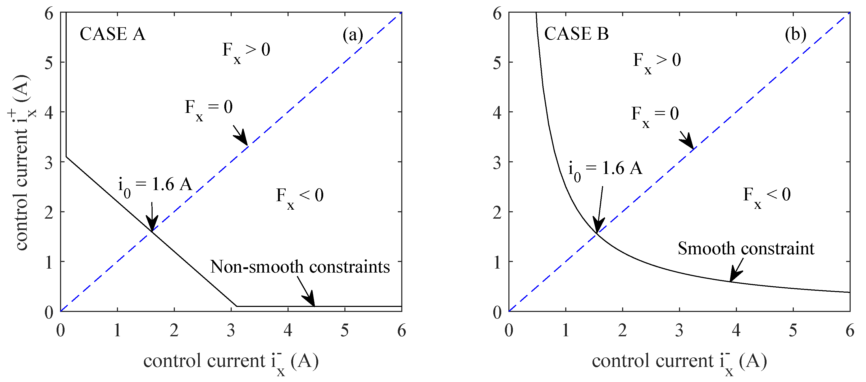
3.1. Gradient-Based Numerical Solution

Defining $\mathit{i}={\left[\begin{array}{cccc}{i}_x^{+}& i_x^{-}& i_y^{+}& i_y^{-}\end{array}\right]}^T$, the force Equations (5) and (6) can be expressed in quadratic matrix form as

$$\mathit{F}\left(\mathit{i}\right)=\left[\begin{array}{c}{F}_x\\ F_y\end{array}\right]=\frac{1}{2}\left[\begin{array}{c}{\mathit{i}}^T{\mathit{H}}_x\mathit{i}\\ {\mathit{i}}^T{\mathit{H}}_y\mathit{i}\end{array}\right]$$

(7)

where

$${\mathit{H}}_x=\left[\begin{array}{cccc}2a_5& 0& a_1& a_2\\ 0& 2a_6& a_3& a_4\\ a_1& a_3& 2a_7& 0\\ a_2& a_4& 0& 2a_8\end{array}\right],{\mathit{H}}_y=\left[\begin{array}{cccc}2b_5& 0& b_1& b_2\\ 0& 2b_6& b_3& b_4\\ b_1& b_3& 2b_7& 0\\ b_2& b_4& 0& 2b_8\end{array}\right]$$

(8)

Further, the Jacobian (derivative) matrix may be obtained, with respect to $\mathit{i}$, as

$$\mathit{J}\left(\mathit{i}\right)=\left[\begin{array}{c}{\mathit{i}}^T{\mathit{H}}_x\\ {\mathit{i}}^T{\mathit{H}}_y\end{array}\right]$$

(9)

An algorithm to perform iterative updates of $\mathit{i}$ must produce convergence of $\mathit{F}\left(\mathit{i}\right)$ to the target force values ${\mathit{F}}_c={\left[\begin{array}{cc}{F}_{cx}& F_{cy}\end{array}\right]}^T$, which are produced in real time by the feedback control algorithm. As there are four independent variables and only two force components, two more constraints may be introduced. By defining these constraints in the general form $\mathit{g}\left(\mathit{i}\right)=0$, they may be incorporated within an extended error vector, as given by

$${\tilde{\mathit{e}}}_n=\left[\begin{array}{c}\mathit{F}\left({\mathit{i}}_n\right)-{\mathit{F}}_c\\ \mathit{g}\left({\mathit{i}}_n\right)\end{array}\right]$$

(10)

where ${\mathit{i}}_n$ is the $n\mathrm{th}$ solution update. Hence, if ${\tilde{\mathit{e}}}_n=0$, the required force value is achieved and the current constraints are satisfied. The corresponding Jacobian matrix has dimensions $4\times 4$:

$${\tilde{\mathit{J}}}_n=\left[\begin{array}{c}\mathit{J}\left({\mathit{i}}_n\right)\\ \nabla {\mathit{g}}^T\left({\mathit{i}}_n\right)\end{array}\right]$$

(11)

An update equation based on a Newton iteration with step length $\alpha$ is given by:

$${\mathit{i}}_{n+1}={\mathit{i}}_n-\alpha {\tilde{\mathit{J}}}_n^{-1}{\tilde{\mathit{e}}}_n$$

(12)

This iteration must be repeated multiple times within each control update until $∥{\tilde{\mathit{e}}}_n∥<ϵ$ with some predefined tolerance $ϵ$. Generally, the solution from the previous time step can be used as the initial solution for the present time step, thereby speeding convergence. Alternatively, the solution obtained by a linear approximation model (see Section 3.2) can be used to initialize the algorithm. For the versions of the algorithm implemented and tested here, constraints were adopted in the form

$$\mathit{g}\left(\mathit{i}\right)=\left[\begin{array}{c}{g}_x(i_x^{+},i_x^{-})\\ g_y(i_y^{+},i_y^{-})\end{array}\right]=0$$

(13)

Two cases are shown in Figure 4. For case A, the constraints involve three line segments and are equivalent to a differential driving mode with bias current $i_0$ and lower saturation limit $i_{min}$. For this case, the corresponding constraint functions may be defined as

$$g_x(i_x^{+},i_x^{-})=\left\{\begin{array}{cc}{i}_x^{+}-i_{min},\hfill & i_x^{-}>2i_0-i_{min}\hfill \\ i_x^{-}-i_{min},\hfill & i_x^{+}>2i_0-i_{min}\hfill \\ i_x^{-}+i_x^{+}-2i_0,\hfill & \mathrm{otherwise}\hfill \end{array}\right.$$

(14)

The corresponding vectors of derivatives are

$$\nabla g_x^T=\left\{\begin{array}{cc}\left[\begin{array}{cccc}1& 0& 0& 0\end{array}\right],\hfill & i_x^{-}>2i_0-i_{min}\hfill \\ \left[\begin{array}{cccc}0& 1& 0& 0\end{array}\right],\hfill & i_x^{+}>2i_0-i_{min}\hfill \\ \left[\begin{array}{cccc}1& 1& 0& 0\end{array}\right],\hfill & \mathrm{otherwise}\hfill \end{array}\right.$$

(15)

and similarly for $g_y(i_y^{+},i_y^{-})$.

With this scheme, a key benefit of using a non-zero bias value $i_0$ is maintained i.e., the operating point $i_x^{+}=i_x^{-}=0$ is avoided, thereby preventing loss of controllability associated with the Jacobian becoming singular. In practical terms, the slope of $\mathit{F}\left(\mathit{i}\right)$ becomes too small leading to unachievably high current slew-rates [11]. The sum (mean value) of the currents is set by the value of $i_0$, while linear operation of the bearing is maintained through the solution of the inverse model. As the force-current relation is quadratic and the constraint are linear in this case, the update algorithm is guaranteed to converge for sufficiently small step-size $\alpha$ provided the Jacobian remains non-singular. By substituting (12) in (10), the error convergence equation is obtained as

$${\tilde{\mathit{e}}}_{n+1}=(1-\alpha ){\tilde{\mathit{e}}}_n+\frac{1}{2}{\alpha }^2\left[\begin{array}{c}{\tilde{\mathit{e}}}_n^T{\mathit{J}}_n^{-T}{\mathit{H}}_x{\mathit{J}}_n^{-1}{\tilde{\mathit{e}}}_n\\ {\tilde{\mathit{e}}}_n^T{\mathit{J}}_n^{-T}{\mathit{H}}_y{\mathit{J}}_n^{-1}{\tilde{\mathit{e}}}_n\\ 0\\ 0\end{array}\right]$$

(16)

Consequently, with step length $0<\alpha \le 1$ a sufficient condition for $\left|{\tilde{\mathit{e}}}_{n+1}\right|<\left|{\tilde{\mathit{e}}}_n\right|$ is

$$\alpha <2\left|{\left(e_{x,y}\right)}_n\right|{\left|{\tilde{\mathit{e}}}_n^T{\mathit{J}}_n^{-T}{\mathit{H}}_{x,y}{\mathit{J}}_n^{-1}{\tilde{\mathit{e}}}_n\right|}^{-1}$$

(17)

where $e_{x,y}$ are the force error components. Although a step length can be chosen based on this bound, faster convergence may be achieved by using an adaptive step length. This is done by initially setting $\alpha =1$. Then, if an update produces an increase in the error, the step length is halved and the solution recalculating. Whereas, if a solution reduces the error, the step length can be doubled subject to $\alpha \le 1$.

This numerical solution approach is suitable for other cases based on more complex models that take account of magnetic flux saturation, or constraints that involve nonlinear functions. However, the convergence properties should be checked thoroughly before any real application is attempted. For further investigation, a case with hyperbolic constraints is considered, as shown by Case B in Figure 4b, where

$$g_x(i_x^{+},i_x^{-})=(i_x^{+}-i_{min})(i_x^{-}-i_{min})-{(i_0-i_{min})}^2=0$$

(18)

$$g_y(i_y^{+},i_y^{-})=(i_y^{+}-i_{min})(i_y^{-}-i_{min})-{(i_0-i_{min})}^2=0$$

(19)

As for Case A, the mean value of the currents satisfies $i_x^{+}+i_x^{-}\ge 2i_0$, but there is no hard saturation of the currents, and instead $i_x^{+}\to i_{min}$ as $i_x^{-}\to \infty$ and vice-versa. The corresponding vectors of gradients for the update algorithm are

$$\nabla g_x^T=\left[\begin{array}{cccc}{i}_x^{-}-i_{min}& i_x^{+}-i_{min}& 0& 0\end{array}\right]$$

(20)

$$\nabla g_y^T=\left[\begin{array}{cccc}0& 0& i_y^{-}-i_{min}& i_y^{+}-i_{min}\end{array}\right]$$

(21)

3.2. Linear Approximation Solution

For the DAMB driving scheme, a more conventional approach can be adopted that involves operating point linearization with fixed bias currents. For this approach, we consider the truncated Taylor series for $F_x$ and $F_y$ about an operating point (OP) with $\mathit{i}={\mathit{i}}_0$, $x=0$, $y=0$. Hence, the x component of the bearing force is

$$F_x=\frac{1}{2}{\mathit{i}}^T{\mathit{H}}_x\mathit{i}\approx \frac{1}{2}{\mathit{i}}_0^T{\left({\mathit{H}}_x\right)}_{\mathrm{OP}}{\mathit{i}}_0+{\mathit{i}}_0^T{\left({\mathit{H}}_x\right)}_{\mathrm{OP}}(\mathit{i}-{\mathit{i}}_0)+\frac{1}{2}{\mathit{i}}_0^T{\left({\nabla }_x{\mathit{H}}_x\right)}_{\mathrm{OP}}{\mathit{i}}_{0}x+\frac{1}{2}{\mathit{i}}_0^T{\left({\nabla }_y{\mathit{H}}_x\right)}_{\mathrm{OP}}{\mathit{i}}_{0}y$$

(22)

Setting $i_x^{+}=i_0+i_x^c$ and $i_x^{-}=i_0-i_x^c$ where $i_0$ is the bias current value, and assuming symmetry of the bearing so that ${\mathit{i}}_0^T{\left({\mathit{H}}_x\right)}_{\mathrm{OP}}{\mathit{i}}_0=0$ and ${\mathit{i}}_0^T{\left({\nabla }_y{\mathit{H}}_x\right)}_{\mathrm{OP}}{\mathit{i}}_0=0$, then (22) simplifies to

$$F_x=K_i^x{i}_x^c+K_s^{x}x$$

(23)

where the current gain and displacement gain take scalar values given by

$$K_i^x={\mathit{i}}_0^T{\left({\mathit{H}}_x\right)}_{\mathrm{OP}}{\left[\begin{array}{cccc}1& -1& 0& 0\end{array}\right]}^T,K_s^x=\frac{1}{2}{\mathit{i}}_0^T{\left({\nabla }_x{\mathit{H}}_x\right)}_{\mathrm{OP}}{\mathit{i}}_0$$

Equivalent equations can be obtained for the y force component and so the required control currents can be calculated directly as $i_x^c={\left(K_i^x\right)}^{-1}{F}_x-{\left(K_i^x\right)}^{-1}{K}_s^{x}x$ and $i_y^c={\left(K_i^y\right)}^{-1}{F}_y-{\left(K_i^y\right)}^{-1}{K}_s^{y}y$. In this calculation, the second term compensates for the negative stiffness of the bearing, while the first term is the additional current required to produce the net force $F_{x,y}$. Clearly, the effectiveness of this approach is dependent on the accuracy of the linear approximation in (22). Moreover, this accuracy will tend to deteriorate as the bias current value is reduced.

4. Experiments

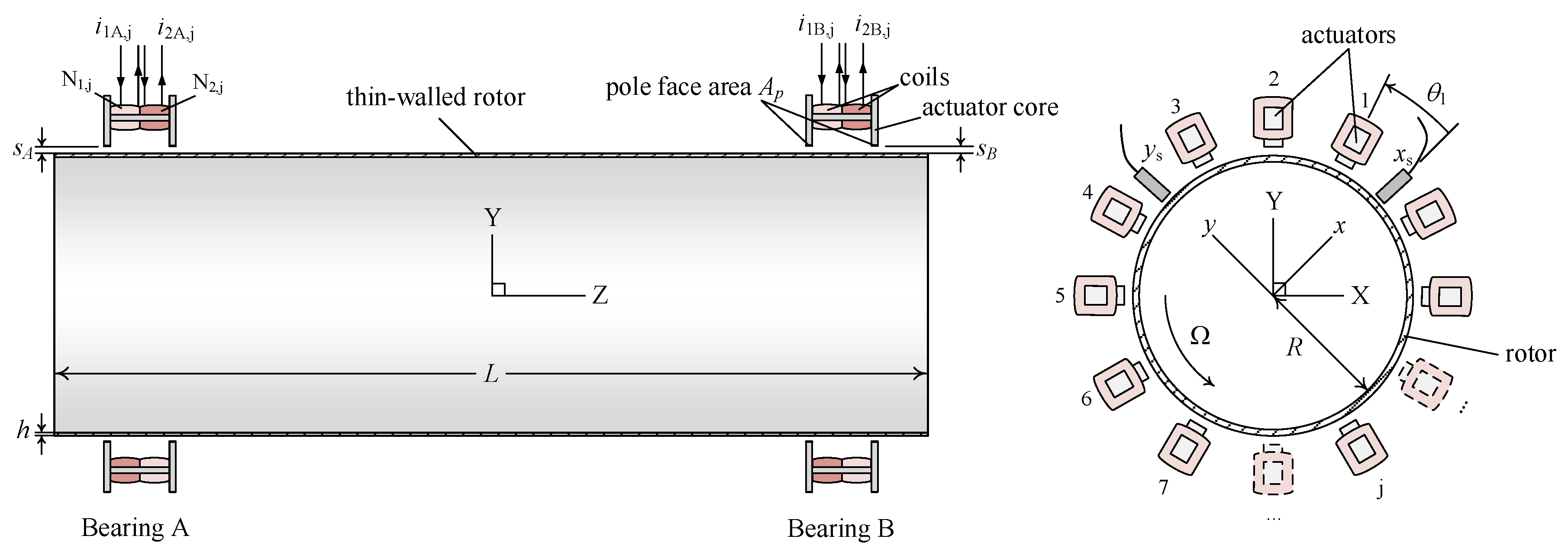
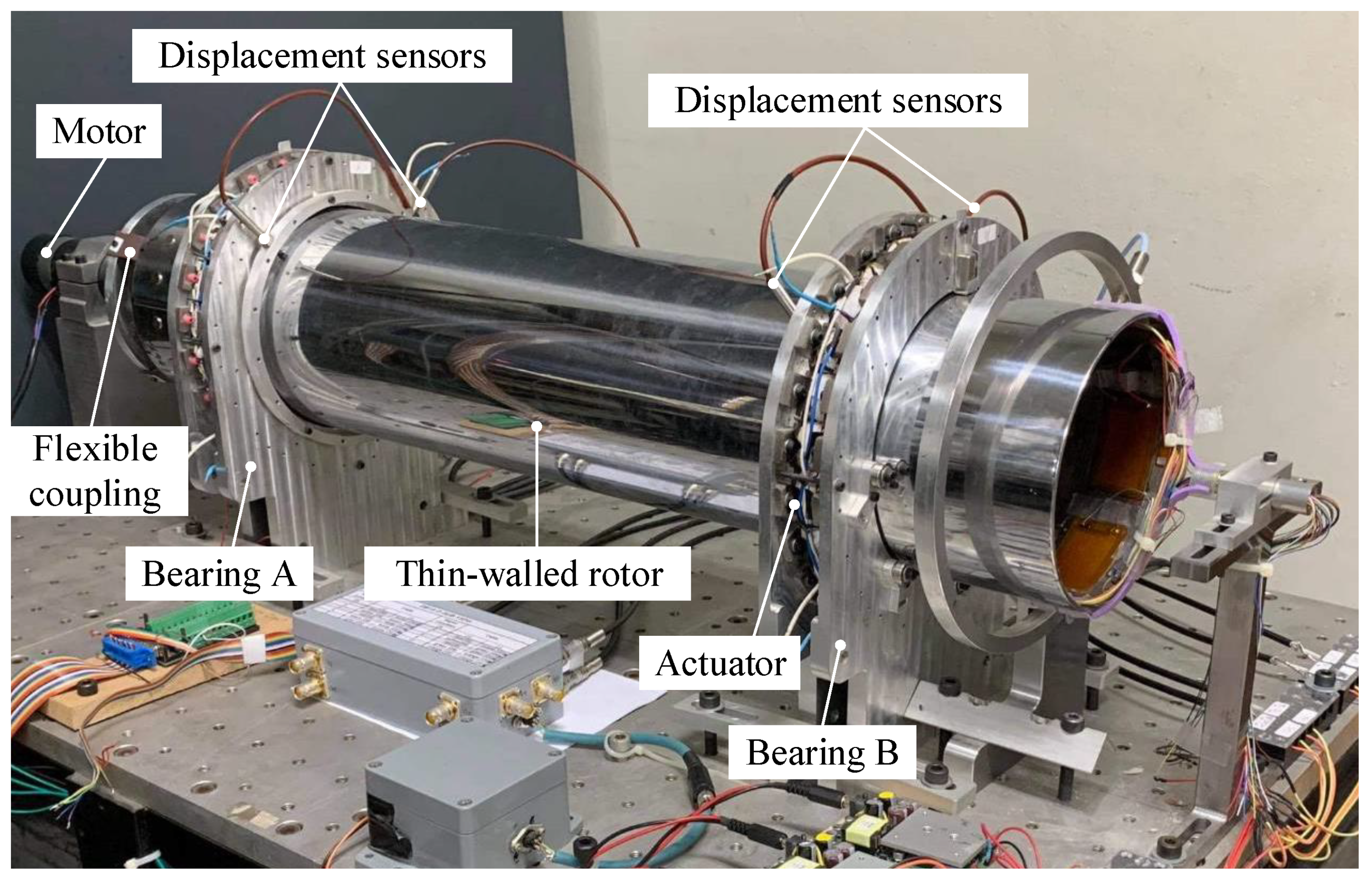
4.1. Thin-Walled Rotor and DAMB Test System

The proposed DAMB design and control approach have been applied to a horizontal cylindrical rotor of length 800 mm with two radial DAMB supports, as shown in Figure 5. The rotor is made from a uniform steel tube with properties given in

Table 2. Physical properties of thin-walled steel rotor.

Parameter	Symbol	Value	Units
Length	L	$0.8$	m
Radius	R	$0.0815$	m
Wall thickness	h	$0.00306$	m
Density	$\rho$	7850	$\mathrm{kg}/{\mathrm{m}}^3$

. Each bearing comprises a circular array of 24 electromagnetic actuators, the design for which is shown in Figure 6. The bearing design parameters are shown in

Table 3. Properties of DAMB actuators.

Parameter	Symbol	Value	Units
Pole face area	$A_p$	$55.8$	mm${}^2$
Permeability of free space	${\mathsf{\mu }}_0$	$4\pi \times {10}^{-7}$	H/m${}^{-1}$
Maximum number of coil-turns	$N_0$	100
Bearing A
Gap size	$s_{0A}$	$0.35$	mm
Effective flux path length	$l_{0A}$	$1.1$	mm
Bearing B
Gap size	$s_{0B}$	$0.2$	mm
Effective flux path length	$l_{0B}$	$0.8$	mm

. The two bearings are configured with different gap sizes but are otherwise identical. The actuator cores are made from soft magnetic powder-sintered steel alloy (Somaloy SPM) to minimize eddy current losses. Each bearing has four sets of actuator coils, in accordance with (4). For each set, the actuator coils are connected in series and driven by a d.c. servo drive (Maxon EC48/5). The variation in the number of turns for each coil is defined by

$$N_{1,j}=\mathrm{round}\left(N_0\frac{\left|cos{\theta }_j\right|}{\sqrt{\left|sin{\theta }_j\right|+\left|cos{\theta }_j\right|}}\right)\mathrm{and}{N}_{2,j}=\mathrm{round}\left(N_0\frac{\left|sin{\theta }_j\right|}{\sqrt{\left|sin{\theta }_j\right|+\left|cos{\theta }_j\right|}}\right)$$

where $N_0$ is the maximum number of coil-turns, as detail in Table 3. This scheme creates a sinusoidal variation in actuator forces around the circumference of the rotor, thereby helping to minimize flexural distortion and vibration of the rotor wall [5].

The rotor is driven by a brushless d.c. motor connected via a flexible coupling, which comprises a disk on the motor shaft and four foam rubber flexures that connect the end of the rotor with the disk in order to transmit torque to the rotor. The flexures have low stiffness in the lateral direction so that the effect of the coupling on the dynamics of the rotor is very low. An orthogonal pair of rotor position sensors (eddy current proximity probes) are located adjacent to each bearing and used for feedback control of the bearings. The feedback control algorithm (including the algorithm for solving the inverse bearing model) is implemented in discrete time on PC-based hardware with the sampling frequency set to 5 kHz.

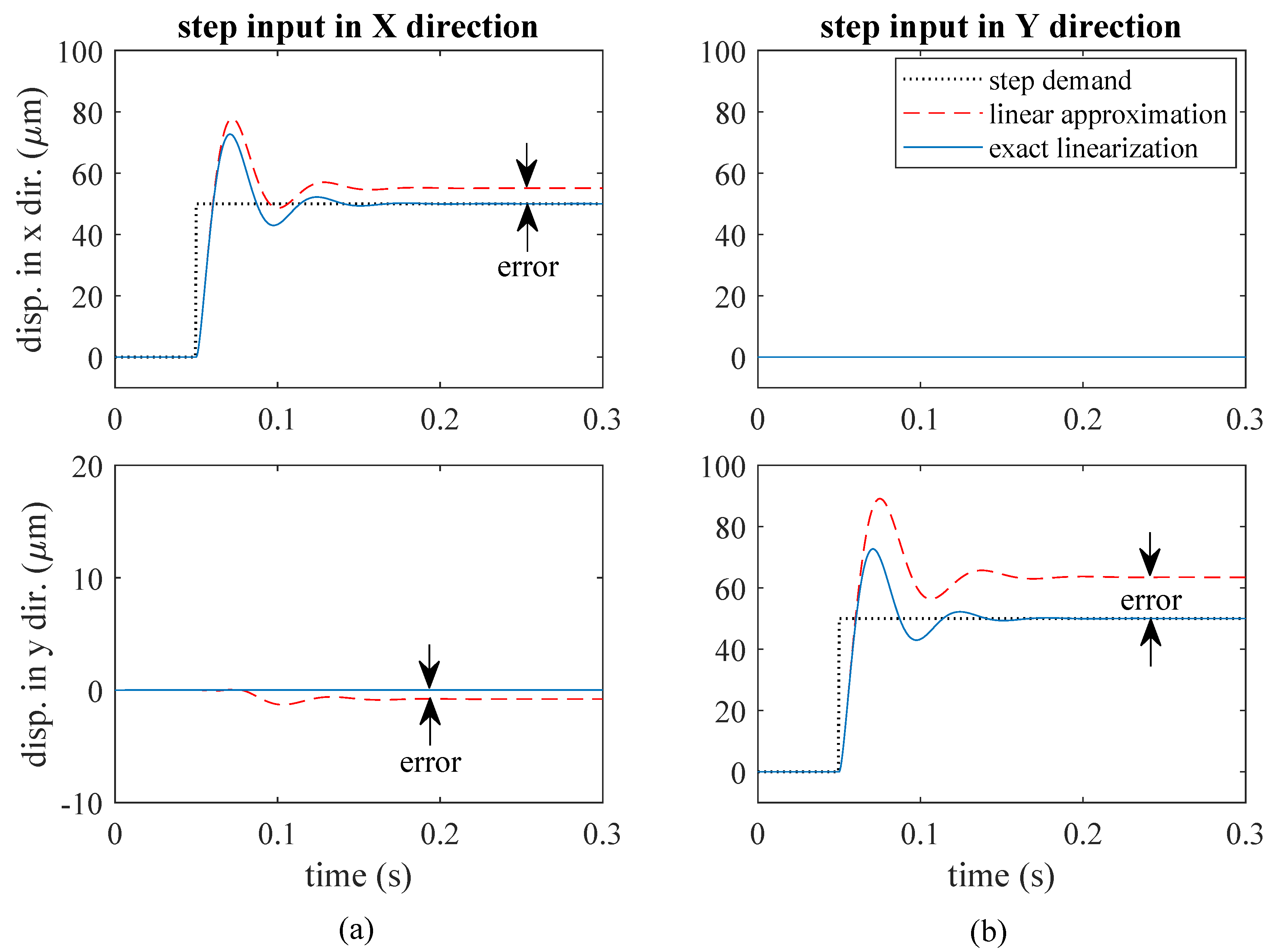
4.2. DAMB Simulations

To verify the convergence properties and correct operation of the linearizing control algorithm, a single bearing was simulated with a 2 d.o.f. lumped mass rotor of 5 kg (which is half the mass of the actual rotor). The DAMB properties were selected to match those of bearing A in Table 3. The bearing force demand was generated via the feedback controller according to the block diagram in Figure 7. Results were obtained to compare the two approaches described in Section 3, which are the exact linearization approach and the linear approximation approach. Step changes in position demand input were simulated with PD feedback control, the results for which are shown in Figure 8. Both cases involve operation with bias current $i_0=1.6$ A and initial position $x=0$ and $y=0$. The controller P and D gains are 70 kN/m and 400 Ns/m respectively. Cases with step changes in horizontal and vertical (X and Y axis) position demand are shown where the bearing axes are aligned at ${45}^{\circ }$ to the vertical (see Figure 3). The gravity force is also included. For the exact linearization approach, the nonlinear negative stiffness property of the bearing is exactly canceled by the inverse model and the transient and steady-state response are the same as if the PD feedback control were applied to the free rotor (as in Figure 2). It can also be seen that there is no cross-coupling between the two axes even though the rotor weight introduces asymmetric loading on the bearing. With the linear approximation approach, significant steady-state error in rotor position occurs following the step in demand. This is because the negative stiffness coefficients from operating point linearization (see (23)) are no longer appropriate following the change in rotor position.

In the implementation of the exact linearization approach, the coil current values are computed using the gradient-based algorithm with hyperbolic constraints. The current values from the linear approximation are used as the initial values ${\mathit{i}}_{\mathrm{init}}$ for the update iterations, as shown in Figure 7. The coil currents, $\mathit{i}$, were calculated via 10 iterations of the root-finding algorithm with fixed step length of $\alpha =$ 0.5 (see (12)). Details on the bearing force calculation for $F_x$ are shown in Figure 9b. It can be seen that the bearing force error converges rapidly and uniformly to the target force value (see Figure 9c). Note that the actual current values are updated only after the 10 iterations are completed. With this algorithm, the bearing force properties can be linearized over the entire operating space of the rotor, thereby eliminating errors for both position and force based control strategies. It should be recognized, however, that these results rely on an exact match between the actual bearing properties and the force model, which is impossible to achieve in practice.

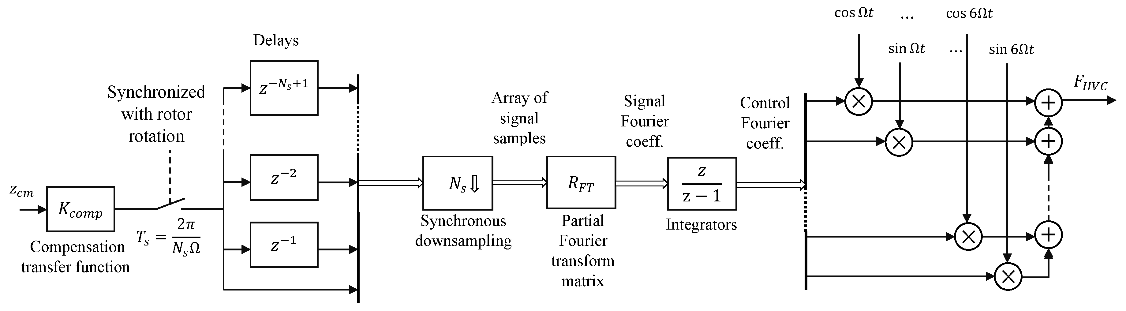
4.3. Practical Implementation

Experiments were undertaken where the inverse bearing model was implemented in the control of the test system described in Section 4.1. The feedback control scheme is shown in Figure 10, where the measured rotor displacements at Bearing A and B are transformed to center-of-mass displacements by transformation matrix ${\mathbf{T}}_{cm}$. Thus, the rotor feedback control is applied in the center of mass coordinate system. The feedback linearization algorithm is applied separately to each bearing based on the local measurements of the rotor displacement within each bearing.

A harmonic vibration control (HVC) algorithm is applied in parallel with the PD controller to eliminate multi-harmonic vibration of the rotor when rotating. Previously, it has been shown that multi-harmonic vibration of a thin-walled rotor is prone to arise due to a combination of mass-unbalance and non-circularity of the rotor wall [6]. In the present study, the HVC is used to eliminate rotor vibration so that the required vibration control forces can be evaluated and compared. The HVC algorithm shown in Figure 11 operates on each center of mass coordinate (which have been decoupled by application of the inverse bearing models). A second order transfer function $K_{comp}$ is first applied to compensate for the dynamics of the system (i.e., $K_{comp}$ is an approximate inverse model). The signals are then down-sampled to form a vector of $N_s$ sample values that cover one complete revolution of the rotor. The first six harmonic amplitudes (Fourier coefficients) are then obtained by multiplication with the discrete Fourier transform matrix given by:

$${\mathbf{R}}_{FT}=\frac{1}{N_s}\left[\begin{array}{ccccc}1& cos\theta & cos2\theta & \cdots & cos(N_s-1)\theta \\ 0& sin\theta & sin2\theta & \cdots & sin(N_s-1)\theta \\ ⋮& & & \ddots & ⋮\\ 1& cos6\theta & cos12\theta & \cdots & cos6(N_s-1)\theta \\ 0& sin6\theta & sin12\theta & \cdots & sin6(N_s-1)\theta \end{array}\right]\mathrm{where}\theta =2\pi /N_s$$

The resulting coefficients are then integrated on a cycle-by-cycle basis and the control signal $F_{HVC}$ formed as a summation of harmonic signals multiplied by the corresponding Fourier coefficients.

Initial tests were performed involving step changes in X and Y position demand for the rotor center of mass, where the X and Y axes align with the horizontal and vertical directions respectively. Figure 12 shows the results for tests with step change in position demand of 50 $\mathsf{\mu }\mathrm{m}$, and with P and D gains of 140 kN/m and 1000 Ns/m respectively for the X and Y coordinates. The bias current values were $i_0=1.6$ A. The transient response with exact linearization is seen to match well with expected behavior. Based on the linear free-rotor model and PD controller gains, the expected values of natural frequency and damping ratio are 118 rad/s and 0.42, respectively. The damping levels are slightly lower than expected due to lag effects within the control loop, which are not accounted for within the inverse bearing model. For the case with feedback control based on the linear approximation model, much larger positioning error occurred. Additionally, for large Y-axis motions (see Figure 12b), the rotor response is prone to instability. Note also that cross-coupling effects are significantly reduced with the exact linearization approach (see Figure 12a). These results are in broad agreement with the simulation results in Figure 8. However, exact linearization cannot be achieved in practice. This is believed to be due to the simplifications within the magnetic force model (Equation (3)). It is known that the main causes of error with this type of model are flux leakage and non-uniform field effects, as well as nonlinear B-H properties of the core materials [18]. The results here indicate that the negative stiffness property of the bearing tends to be underestimated with both the exact linearization and linear approximation models.

To further examine the position-dependent force characteristics of the bearings, tests were undertaken involving sinusoidal tracking for the rotor center of mass position. The tests involved a low frequency (2 rad/s) sine wave demand with amplitude of 50 $\mathsf{\mu }\mathrm{m}$. Exact compensation of the position-dependency of the bearing force would lead to exact tracking in these tests as inertia effects are negligible. Figure 13 shows that for the linear approximation model, the position error increases significantly as the rotor moves away from the operation point ($x=0\mathsf{\mu }\mathrm{m}$ and $y=0\mathsf{\mu }\mathrm{m}$). With the exact linearization approach, the positioning error and axis cross-coupling is greatly reduced.

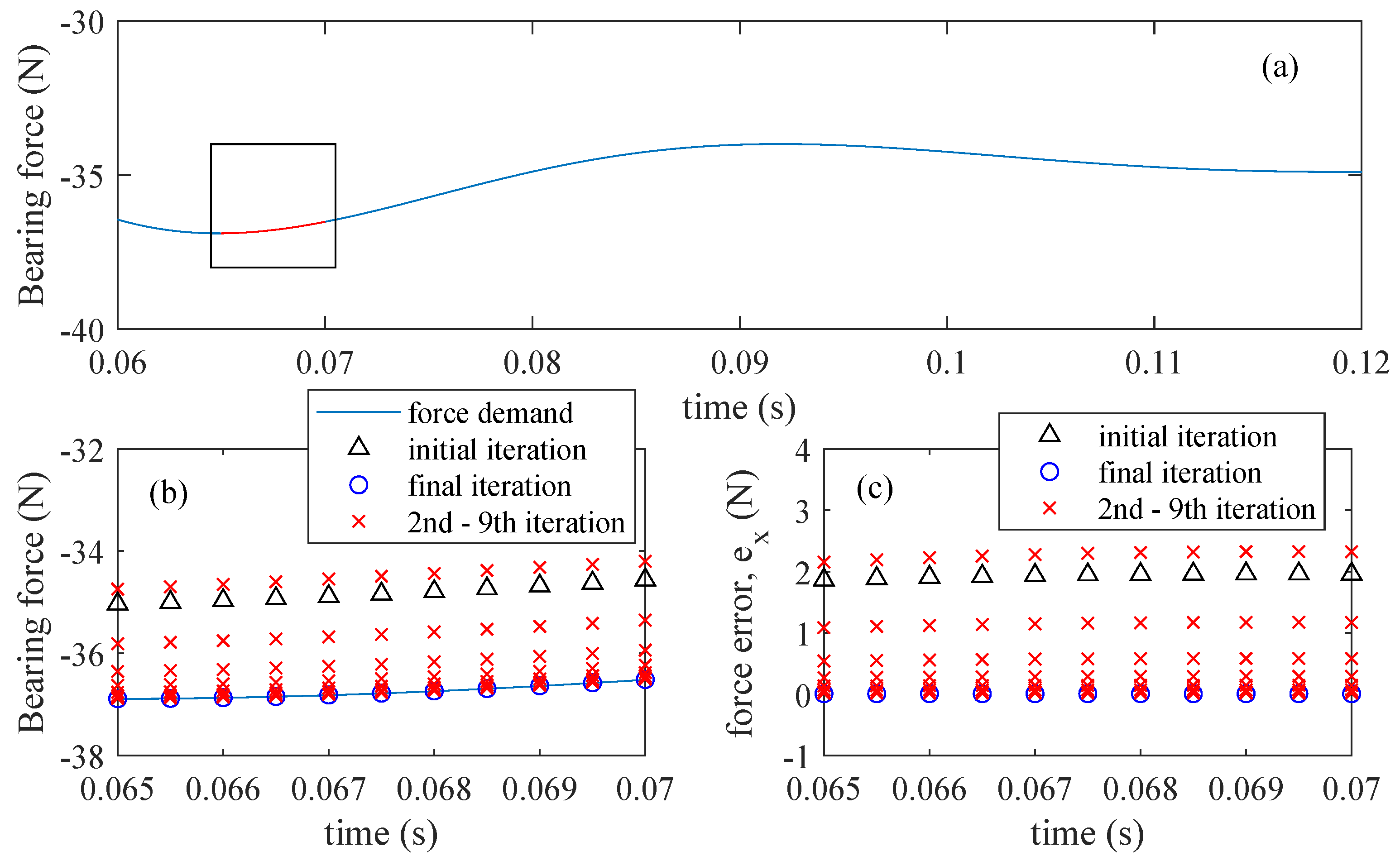
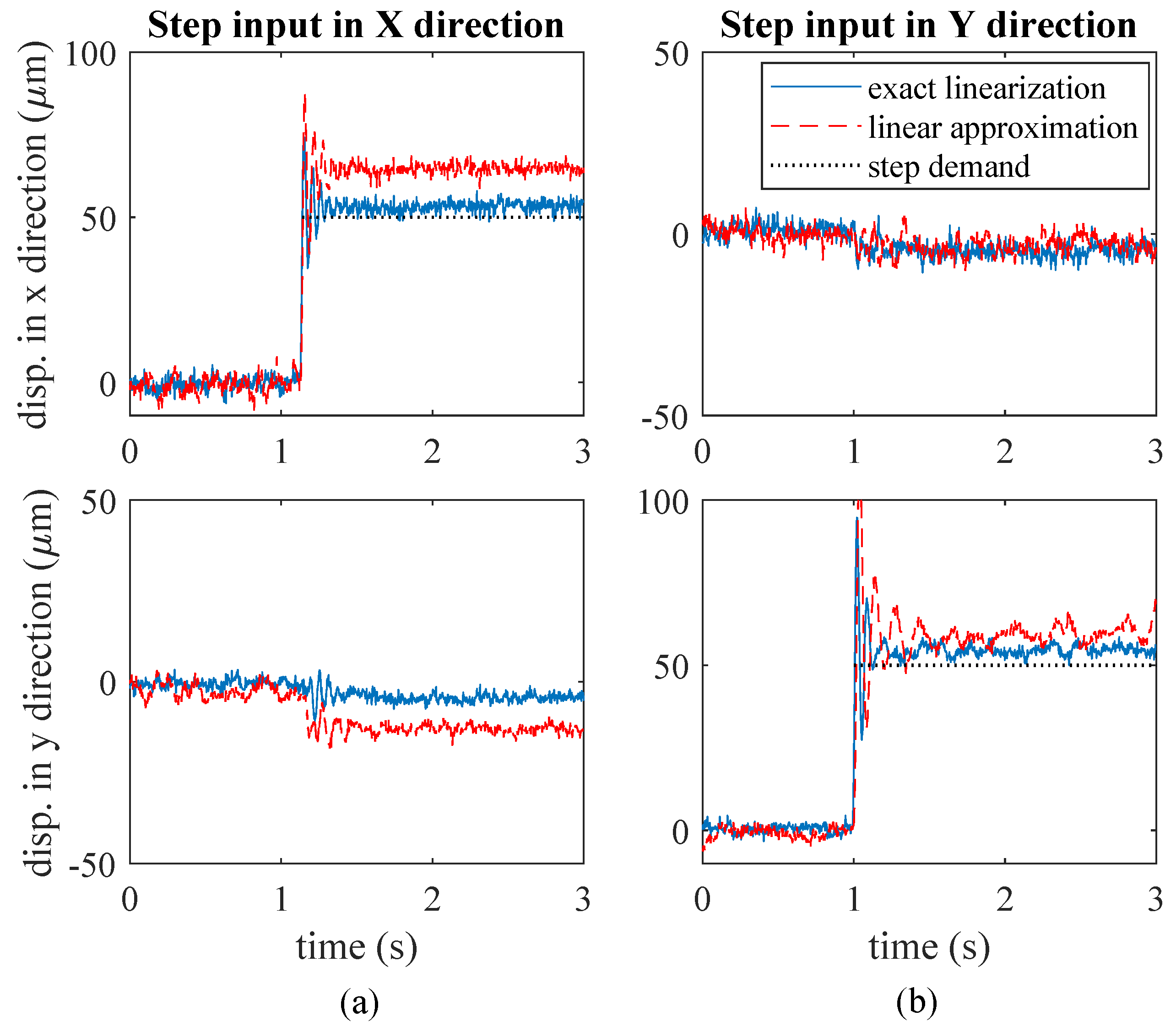
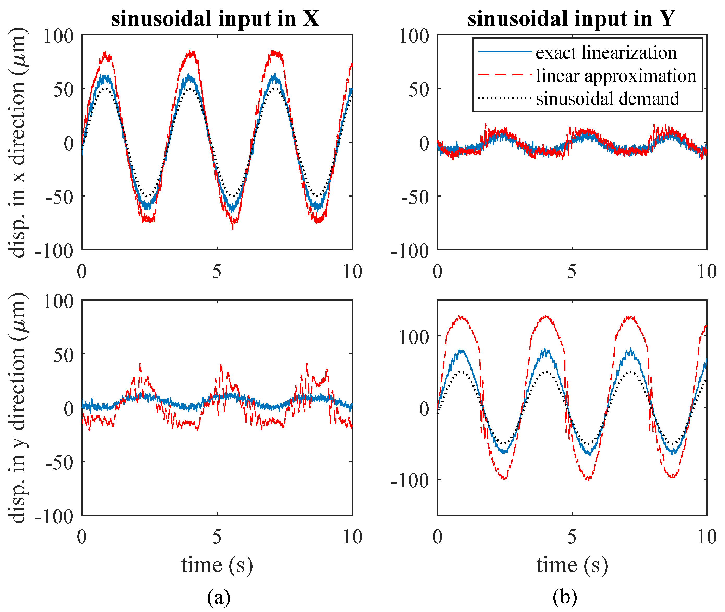
4.4. DAMB Force Control Evaluations

To further evaluate the force properties of the bearing and accuracy of the inverse model, tests with rotation were conducted where control forces were applied to eliminate vibration of the rotor. These tests were performed at relatively low speeds, but with large added unbalance, in order to minimize errors due to the finite bandwidth of the current control loops and other lag effects within the feedback control loop. Feedback control with exact linearization was implemented in combination with HVC control so that the vibration of the rotor can be reduced and the synchronous component eliminated, as shown in Figure 14a. Stable operation of the bearings using the exact linearization algorithm with hyperbolic current constraints (bias $i_0=1.6$ A) is achieved despite large differences in the coil current values. For comparison purposes, results from operation with the linear approximation controller with synchronous (unbalance) control only are shown in Figure 14b. To achieve stable operation of the bearing, the bias current value was increased to 2.2 A. Significant vibration of the rotor involving higher harmonics of the rotational frequency occurred for this case. This vibration is caused by noncircularity of the rotor cross-section, as well as nonlinear effects from the bearing (see Reference [6]). The effectiveness of the control implementations can be further compared from Figure 15, where Fourier transform data for the rotor vibration signals and coils currents are presented. A reduction in both mean and RMS values of the AMB currents is achieved with the proposed control implementation, in addition to the large reduction in rotor vibration.

As synchronous vibration of the rotor is practically eliminated in these tests, the synchronous force from the bearings should exactly match the mass-unbalance of the rotor. Hence, the predicted bearing force from the inverse model can be used to estimate the unbalance of the rotor. To evaluate the accuracy of the force prediction, the unbalance force was estimated for cases with and without an unbalance mass of 97 grams applied at the middle inner surface of the rotor (angular position 0 degree) such that the mass-eccentricity was 0.0074 kg-m.

Table 4. Unbalance estimation results from nonlinear force model: actual unbalance was $0.0074$∠$0^{\circ }$.

Rotational Frequency (rad/s)	Estimated Force (N∠deg)	Estimated Unbalance (kg·m∠deg)
$19.0$	$2.57\angle {2.3}^{\circ }$	$0.0071\angle {2.3}^{\circ }$
$25.1$	$4.68\angle {0.3}^{\circ }$	$0.0074\angle {0.3}^{\circ }$
$31.2$	$7.38\angle {-1.7}^{\circ }$	$0.0076\angle {-1.7}^{\circ }$

shows the estimates of the unbalance force obtained during operation and the corresponding mass-eccentricity estimate for rotational frequencies of 19.0 rad/s, 25.1 rad/s and 31.2 rad/s. The results confirm that the unbalance force prediction from the inverse bearing model matches the actual unbalance well over the range of force levels tested.

5. Conclusions

This paper has introduced an exact linearizing control approach for a distributed actuation magnetic bearing supporting a thin-walled rotor. As the set of coupled nonlinear equations that relate bearing forces to coil currents cannot be solved analytically, for control purposes, a method for numerical solution of the equations in real-time has been proposed. Accurate solutions could be obtained during each feedback control update using a finite number of Newton iterations for the coil current values. Moreover, the formulation can incorporate arbitrary constraint equations for the coil currents. This can be exploited to achieve low mean current values, while minimizing nonlinear effects. Experiments conducted on a thin-walled rotor with two DAMB supports showed that the linearizing and decoupling properties of the control implementation allow effective vibration control to be achieved with lower currents and with improved performance compared with standard control methods based on linear approximation models. For the experimental system, force errors arose mainly due to inaccuracy of the considered magnetic flux model, which did not account for flux leakage or saturation effects. Nonetheless, the method has general applicability and can be applied with more complex nonlinear models of force behaviour in AMB systems.

References

1. Schweitzer, G.; Bleuler, H.; Maslen, E.; Cole, M.; Keogh, P.; Larsonneur, R.; Maslen, E.; Nordmann, R.; Okada, Y. Magnetic Bearings: Theory, Design, and Application to Rotating Machinery; Springer: Berlin/Heidelberg, Germay, 2009. [Google Scholar]
2. Xu, X.; Chen, S. Field Balancing and Harmonic Vibration Suppression in Rigid AMB-Rotor Systems with Rotor Imbalances and Sensor Runout. Sensors 2015, 15, 21876–21897. [Google Scholar] [CrossRef] [PubMed] [Green Version]
3. Schneeberger, T.; Nussbaumer, T.; Kolar, J.W. Magnetically Levitated Homopolar Hollow-shaft Motor. IEEE/ASME Trans. Mechatron. 2010, 15, 97–107. [Google Scholar] [CrossRef]
4. Lusty, C.; Sahinkaya, N.; Keogh, P. A Novel Twin-Shaft Rotor Layout with Active Magnetic Couplings for Vibration Control. Proc. IMechE Part I: J. Syst. Control Eng. 2016, 230, 266–276. [Google Scholar] [CrossRef] [Green Version]
5. Cole, M.O.T.; Fakkaew, W. An Active Magnetic Bearing for Thin-Walled Rotors: Vibrational Dynamics and Stabilizing Control. IEEE/ASME Trans. Mechatron. 2018, 23, 2859–2869. [Google Scholar] [CrossRef]
6. Chamroon, C.; Cole, M.O.T.; Fakkaew, W. Model and Control System Development for a Distributed Actuation Magnetic Bearing and Thin-Walled Rotor Subject to Noncircularity. ASME J. Vib. Acoust. 2019, 141, 051006. [Google Scholar] [CrossRef]
7. Zhou, L.; Li, L. Modeling and Identification of a Solid-Core Active Magnetic Bearing Including Eddy Currents. IEEE/ASME Trans. Mechatron. 2016, 21, 2784–2792. [Google Scholar] [CrossRef]
8. Daoud, M.I.; Abdel-Khalik, A.S.; Massoud, A.; Ahmed, S.; Abbasy, N.H. A Design Example of an 8-Pole Radial AMB for Flywheel Energy Storage. In Proceedings of the 2012 XXth International Conference on Electrical Machines, Marseille, France, 2–5 September 2012; pp. 1153–1159. [Google Scholar] [CrossRef]
9. Wei, C.; Soffker, D. Optimization Strategy for PID-Controller Design of AMB Rotor Systems. IEEE Trans. Control Syst. Technol. 2016, 24, 788–803. [Google Scholar] [CrossRef]
10. Zheng, S.; Li, H.; Han, B.; Yang, J. Power Consumption Reduction for Magnetic Bearing Systems during Torque Output of Control Moment Gyros. IEEE Trans. Power Electron. 2017, 32, 5752–5759. [Google Scholar] [CrossRef]
11. Filatov, A.; Hawkins, L.; McMullen, P. Homopolar Permanent-Magnet-Biased Actuators and Their Application in Rotational Active Magnetic Bearing Systems. Actuators 2016, 5, 26. [Google Scholar] [CrossRef] [Green Version]
12. Meeker, D.; Maslen, E. A Parametric Solution to the Generalized Bias Linearization Problem. Actuators 2020, 9, 14. [Google Scholar] [CrossRef] [Green Version]
13. Mazenc, F.; de Queiroz, M.S.; Malisoff, M.; Gao, F. Further Results on Active Magnetic Bearing Control with Input Saturation. IEEE Trans. Control Syst. Technol. 2006, 14, 914–919. [Google Scholar] [CrossRef] [Green Version]
14. Tsiotras, P.; Arcak, M. Low-Bias Control of AMB Subject to Voltage Saturation: State-Feedback and Observer Designs. IEEE Trans. Control Syst. Technol. 2005, 13, 262–273. [Google Scholar] [CrossRef] [Green Version]
15. Gerami, A.; Allaire, P.; Fittro, R. Control of Magnetic Bearing with Material Saturation Nonlinearity. J. Dyn. Syst. Meas. Control 2015, 137, 061002. [Google Scholar] [CrossRef]
16. Chen, S.; Song, M. Energy-Saving Dynamic Bias Current Control of Active Magnetic Bearing Positioning System Using Adaptive Differential Evolution. IEEE Trans. Syst. Man Cybern. Syst. 2019, 49, 942–953. [Google Scholar] [CrossRef]
17. Trumper, D.L.; Olson, S.M.; Subrahmanyan, P.K. Linearizing Control of Magnetic Suspension Systems. IEEE Trans. Control Syst. Technol. 1997, 5, 427–437. [Google Scholar] [CrossRef]
18. Li, L.; Shinshi, T.; Shimokohbe, A. Asymptotically Exact Linearizations for Active Magnetic Bearing Actuators in Voltage Control Configuration. IEEE Trans. Control Syst. Technol. 2003, 11, 185–195. [Google Scholar]
19. Chen, M.; Knospe, C.R. Feedback linearization of active magnetic bearings: Current-mode implementation. IEEE/ASME Trans. Mechatron. 2005, 10, 632–639. [Google Scholar] [CrossRef]
20. Mystkowski, A.; Kaparin, V.; Kotta, U.; Pawluszewicz, E.; Tõnso, M. Feedback linearization of an active magnetic bearing system operated with a zero-bias flux. Int. J. Appl. Math. Comput. Sci. 2017, 27, 539–548. [Google Scholar] [CrossRef] [Green Version]
21. Lindlau, J.D.; Knospe, C.R. Feedback linearization of an active magnetic bearing with voltage control. IEEE Trans. Control Syst. Technol. 2002, 10, 21–31. [Google Scholar] [CrossRef]
Figure 1. Active magnetic bearing suspension incorporating four electromagnetic actuators.
Actuators 09 00099 g001
Figure 2. Rotor-AMB control scheme: (a) with feedback linearization (inverse AMB model) (b) equivalent dynamics.
Actuators 09 00099 g002
Figure 3. Thin-walled rotor with DAMB supports: Cross-section diagrams.
Actuators 09 00099 g003
Figure 4. Examples of current constraints g x ( i x + , i x ) = 0 for use in bearing operation (a) non-smooth constraint (Equation (14)) (b) smooth hyperbolic constraint (Equation (18)).
Actuators 09 00099 g004
Figure 5. Experimental thin-walled rotor with two radial DAMBs.
Actuators 09 00099 g005
Figure 6. Multi-coil actuator for thin-walled rotors (a) schematic (b) solid model.
Actuators 09 00099 g006
Figure 7. Feedback control scheme for exact linearization.
Actuators 09 00099 g007
Figure 8. Simulations of DAMB with lumped-mass rotor for step-change in position demand (a) step input in X direction (b) step input in Y direction.
Actuators 09 00099 g008
Figure 9. Bearing force computation (for F x ) with gradient-based root finding algorithm (a) Bearing force between 0.06 to 0.12 second (b) Bearing force solution updates at each time step (c) Bearing force error updates at each time step.
Actuators 09 00099 g009
Figure 10. Decoupled feedback control scheme with exact linearization.
Actuators 09 00099 g010
Figure 11. Harmonic vibration control algorithm.
Actuators 09 00099 g011
Figure 12. Displacement response of the non-rotating thin-walled rotor due to (a) step change in X demand (b) step change in Y demand.
Actuators 09 00099 g012
Figure 13. Displacement response of the non-rotating thin-walled rotor due to (a) sinusoidal demand input in X direction (b) sinusoidal demand input in Y direction.
Actuators 09 00099 g013
Figure 14. Steady-state behavior of test system at rotational speed of 31.2 rad/s (5 Hz) with (a) exact linearizing control with Harmonic Vibration Control implementation (b) linear approximation control with synchronous (unbalance) control implementation.
Actuators 09 00099 g014
Figure 15. Fourier transforms of displacement and current signals at rotational speed of 31.2 rad/s (5 Hz). Data is shown for x-axis components from each case in Figure 14.
Actuators 09 00099 g015