Enhancing Damage Detection in 2D Concrete Plates: A Comprehensive Study on Interpolation Methods and Parameters

Abstract

In an era marked by increasing demands for stability and durability in construction, the importance of damage detection in concrete structures cannot be overstated. As these structures underpin the safety and longevity of vital assets, this paper embarks on a comprehensive exploration of methodologies to enhance precision and reliability in 2D concrete plate damage detection. By focusing on the interpolation of damage index values and leveraging the insights gained from energy loss analysis and the characterization of the time of arrival of signals, we address the pressing need for improved non-destructive damage detection techniques. Our study encompasses a range of simulation attempts, each involving various interpolation parameters, and systematically evaluates their performance. The culmination of this research identifies the most effective combination of techniques and parameters, leading to the best results in damage detection. This multidimensional investigation promises to provide valuable contributions to the field of structural health monitoring, benefiting both researchers and practitioners engaged in the evaluation of concrete structures.

1. Introduction

Structural health monitoring (SHM) is a crucial tool for comprehensively assessing the performance of a structure. It serves multiple functions, including diagnosing the location and extent of structural damage and intelligently evaluating structural health in terms of usage status, reliability, durability, and carrying capacity. In the presence of adverse conditions, such as structural damage or abnormal behavior, the SHM system triggers early warning signals, providing essential guidance and a foundation for informed building maintenance and management decisions.

Recent years have witnessed substantial growth in the realm of SHM, actively contributing to the improved reliability of structures through the advancement of methodologies for damage detection. A key aspect of this progress involves the use of non-destructive methods, which play a pivotal role in the early identification of structural impairments without causing any destructive impact on the structures themselves. Despite offering valuable insights into structural conditions, these non-destructive methods often require information about the healthy states of a structure as a reference for comparative analysis with the current state obtained through nondestructive evaluation.

In the domain of SHM, a diverse array of methodologies is employed to safeguard the integrity and functionality of various structures. These approaches encompass techniques leveraging acoustic emissions [1], vibration analysis [2], laser scanning [3], and the propagation of ultrasonic waves [4]. Acoustic emissions, for instance, primarily arise from the sudden release of energy within stressed materials, giving rise to transient elastic waves. This phenomenon intricately corresponds to numerous fracture or deformation processes within the material, including crack initiation and propagation, microstructural separation, and material phase displacement [5]. Conversely, vibration analysis serves as a crucial method, where the amplitude of transmitted signals plays a pivotal role in extracting valuable insights into the structural condition. Furthermore, the emerging integration of machine learning and artificial intelligence techniques in the field of SHM holds the potential for improving damage localization accuracy by leveraging vast amounts of data and learning complex patterns. This can be observed in the research conducted by [4] where a machine learning (ML)-based damage detection method is presented. This method utilizes aggregated baselines independent of their damaged states to enhance the generalization capability of ML algorithms by considering similar structural characteristics. Through the application of these diverse methodologies, SHM strives to offer comprehensive monitoring and assessment, thereby enhancing safety and performance across a spectrum of engineering applications. Other innovative methodologies combine non-contact sensors, such as interferometric radar sensors, with finite element modeling. Such methods have shown promising results in accurately capturing the dynamic behavior of structures under various loading conditions. One notable study using this technique investigated the dynamic performance of bridge bearings by capturing the real-time dynamic behavior of the bridge under traffic loading, including key dynamic characteristics such as natural frequencies, which are sensitive indicators of structural integrity [6,7]. In addition to bridge bearings, another study focused on damage identification metrics for smart beams equipped with piezoelectric elements for SHM [8]. This investigation presents a comprehensive analysis of damage identification metrics and their performance. The study highlights the significance of piezoelectric patches in SHM and explores the use of computational models and experimental testing to assess structural damage and stiffness changes in beams. Such implementations enhance the effectiveness of bridge monitoring systems and improve maintenance practices to ensure the continued safety and performance of bridge infrastructure.

SHM serves as a cornerstone in ensuring the safety, longevity, and optimal performance of civil infrastructure, mechanical systems, and aerospace structures. A fundamental aspect of SHM is the accurate localization of damage within these structures, which is crucial for timely maintenance and proactive management strategies. However, achieving precise damage localization is a complex task influenced by a multitude of factors. One critical consideration is the strategic placement of sensors or monitoring devices, as demonstrated in [9], where Finite Element Modeling (FEM) is employed to create a mesh model of the structure, distinguishing between stressed and unstressed zones. Leveraging FEM outcomes, the study identifies optimal sensor positions to maximize coverage within a limited sensor count.

Environmental conditions, such as temperature fluctuations, introduce additional challenges by influencing structural behavior and signal characteristics. Several studies in the field of structural health monitoring have investigated the influence of temperature variations on damage detection methodologies. For instance, a novel approach was proposed in [10] to examine damage localization and quantification in structures subjected to changing temperature conditions. The findings highlight the challenge posed by temperature fluctuations, which can alter the vibration properties of structures and complicate the creation of accurate baselines for damage detection. By employing a single temperature condition as a baseline and utilizing a two-stage approach involving Finite Element Modeling (FEM), the influence of temperature changes was successfully eliminated, and precise damage locations and extents were identified.

The inherent complexity of structures, characterized by geometric intricacies, material heterogeneity, and structural connections, presents significant challenges for accurate damage localization. Various types and severities of damage manifest distinct signatures, further complicating the localization process. Depending on the severity of the damage, different methodologies must be employed. For instance, in the case of detecting extensive damage in structures, image segmentation techniques, coupled with suitable neural networks [11], can effectively identify scenarios like wall collapses. Conversely, when dealing with sensitive structures, where even minor damages are of concern, more sensitive detection methods are required. In such cases, ultrasonic wave propagation techniques, as demonstrated by [12], offer a more suitable approach, leveraging vibration response-based techniques.

Noise in measurement signals, stemming from sensor inaccuracies or environmental interference, significantly hampers the clarity of damage signatures, thus compromising the accuracy of localization efforts. This noise, whether originating from sensor malfunctions or external factors such as vibrations or electromagnetic interference, poses a substantial challenge in distinguishing genuine damage-induced changes from background fluctuations. Addressing this issue requires robust signal processing techniques and meticulous sensor calibration to filter out noise while retaining relevant structural information. Additionally, strategic sensor placement and shielding measures can minimize the impact of environmental interference, ensuring more reliable and accurate damage localization outcomes. An experimental analysis by [13] highlighted the effects of external vibration and noise on SHM applications based on the EMI method, emphasizing the critical nature of these challenges in structural diagnosis. Their findings underscored the significant impact of noise and vibration on impedance signatures and damage indices, necessitating the development of advanced signal processing techniques and more effective indices for damage detection under real-world conditions.

Commencing with advancements in data fusion techniques, which seamlessly integrate data from multiple sensors or measurement methods, the field of SHM has witnessed a remarkable stride toward enhancing localization precision. For instance, as an example application of this field, one technique was utilized to establish a relatively coarse actuator/sensor (AS) network. As the process advances, targeted refinement of the AS network in regions suspected of damage further augments localization precision [14]. This fusion of data methodologies not only propels the accuracy of damage detection but also heralds a new era in optimizing SHM practices.

In light of these multifaceted challenges, this paper aims to explore and address the various factors influencing damage localization within SHM frameworks. Specifically, it investigates the effect of PZT sorting and iterating techniques on 2D damage localization within concrete structures. Moreover, this study endeavors to enhance the previously developed method [15,16] by introducing the alpha interpolation technique, which is a novel contribution. While the previous work utilized a different approach, iterating along the transducers to consider all possible connections between them as AS paths, the introduction of the alpha interpolation method aims to improve damage localization accuracy within SHM contexts. Our proposed method achieves maximum area coverage with minimal overlap, thus enhancing the accuracy of damage detection.

In this paper, the hybrid damage detection method proposed in our previous research [15,16] is further refined through the incorporation of the alpha interpolation method. This refinement aims to enhance the accuracy of damage detection and localization. The characteristics and prerequisites for applying the alpha interpolation method are detailed through several consecutive examples, all of which are implemented on numerical models of a 2D concrete plate. The first parameter of interest is the interpolation mechanism used within the hybrid method. The subsequent investigation focuses on the newly introduced alpha interpolation method, including the determination of the considered area for each interpolation round. Additionally, the impact of averaging accumulated Damage Index (DI) values is explored. Finally, the concept of time-gating is integrated into the improved method, with consideration given to four signal truncation scenarios.

The structure of this paper is organized as follows. In Section 1, we examine various applications in the field of SHM and explore the factors influencing damage localization accuracy. Section 2 delineates the process of determining theoretical Time-of-Arrival (ToA), introduces the concept of time-gating, and conducts a conceptual comparison between the recent interpolation method and the developed alpha interpolation method for damage localization in 2D. Moving on, Section 3 details the model inputs and characteristics, while also presenting supporting examples of the developed method. These examples encompass the effect of different damage location and size criteria, interpolation areas, and the influence of various signal truncation policies on damage localization accuracy. Subsequently, Section 4 elucidates the findings resulting from the improvements in the damage detection strategy. Finally, in Section 5, we highlight the major contributions of this paper and provide suggestions for future research in the field of SHM.

2. Methodology

The method considered in this paper is a modified version of the damage localization method developed by our group [16]. The common idea is that signal propagation is sent within a specimen iteratively at different points on the surface of it. Then each signal is recorded on other predefined points, which are also located on the surface. The recorded signals will be post-processed to get rid of possible noise. After that, the energy loss between a reference state of the specimen and the measured state (damaged state) is used to obtain the one-dimensional $DI$ for each Actuator/Sensor path (AS path). Finally, all the calculated $DI$ values are utilized to detect the existence and location of the damage by applying a specific interpolation technique.

2.1. 1D Damage Index Implementation

The implementation of the one-dimensional $DI$ is achieved using the energy difference between the undamaged and damaged states of the specimen. The $DI$ is defined as the root mean square deviation (RMSD) method [15]. Furthermore, every input signal undergoes decomposition into sets using n-level wavelet decomposition, employing the Daubechies wavelet db9 as the mother wavelet. The rationale behind choosing this specific mother wavelet stems from its proficiency in precisely localizing signal characteristics and demonstrating consistent properties [17]. These characteristics render it highly suitable for analyzing signals that encompass discontinuities and spikes.

The energy of individual waveforms transmitted from a single sender to a single receiver is computed based on decomposed signals. These decomposed signals, denoted by the vector $X_S$, encompass signals at 2ⁿ levels, with each $X_j$ containing $m$ sample data points.

$$X_S=\left\{X_1, X_2, \cdots ,X_j, \cdots , X_{2^{n-1}}, X_{2^n}\right\}$$

(1)

The energy of each decomposed signal, denoted as $E_{\left(.\right), k}$, where $k$ represents the decomposed signal index (with $k=1,\cdots ,2^n$), provides insights into the energy distribution across different states of the specimen (e.g., intact or damaged).

$$E_{\left(.\right), k }={\Vert X_k\Vert }_2^2=x_{k,1}^2+x_{k,2}^2+\cdots +x_{k,m-1}^2+x_{k,m}^2$$

(2)

For each state (intact or damaged), the energy distribution is captured in vectors $E_{h }$ and $E_{d }$, where each element represents the energy of a specific decomposition.

$$E_{h }=E_{h ,1}, E_{h ,2}, \cdots ,E_{h ,2^n}$$

(3)

$$E_{d }=E_{d ,1}, E_{d ,2}, \cdots ,E_{d ,2^n}$$

(4)

Utilizing the Root Mean Square Deviation (RMSD) rule, the Damage Index ($DI$) is calculated as:

$$DI=\sqrt{\frac{{{\displaystyle \sum }}_{p=1}^{2^n}{\left(E_{d,p}-E_{h,p}\right)}^2}{{{\displaystyle \sum }}_{p=1}^{2^n}{E_{h,p}}^2}}$$

(5)

Here, $p$ represents the index of each decomposition level.

The $DI$ ranges between 0 (indicating an undamaged specimen) and 1 (indicating a fully damaged specimen).

2.2. The Concept of the Time-of-Arrival & Time-Gating Technique

As part of the signal processing steps considered in our damage detection method, both the ToA and the time-gating concept are mainly used to obtain useful information on the signals.

2.2.1. The Theoretical Time of Arrival

In our developed approach, the time of arrival criterion holds significant importance as it serves as a primary determinant for assessing the obtained signals. The theoretical time of arrival is derived from the physical attributes of the specimen and the excitation signal, as outlined by the following equation.

$$To{A}_{Theoretical}=\frac{L_{AS}}{v_{max}}$$

(6)

where:

$L_{AS}$: the distance between the actuator (A) and the sensor (S) on the specimen [m].

$v_{max}$: the fastest velocity of the propagated wave ($c_L$ longitudinal velocity) [m/s].

The concrete material defined for this paper is considered an isotropic elastic material. Additionally, the lateral dimensions of the specimens are big enough compared to the wavelength to be considered. Based on these considerations, the longitudinal velocity of the propagated wave is calculated based on the material properties as follows

$$c_L=\sqrt{\frac{\lambda +2\mu }{\rho }}$$

(7)

where the Lame constants ($\mu ,\lambda$) required for the calculation can be acquired depending on the material properties as follows:

$$\mu =\frac{E}{2\left(1+\upsilon \right)}, \lambda =\frac{E\upsilon }{\left[\left(1-2\upsilon \right)\left(1+\upsilon \right)\right]}$$

(8)

where

$E,\upsilon ,\rho$—Young’s modulus, Poisson’s ratio, and material density, respectively.

2.2.2. The Time-Gating Strategy

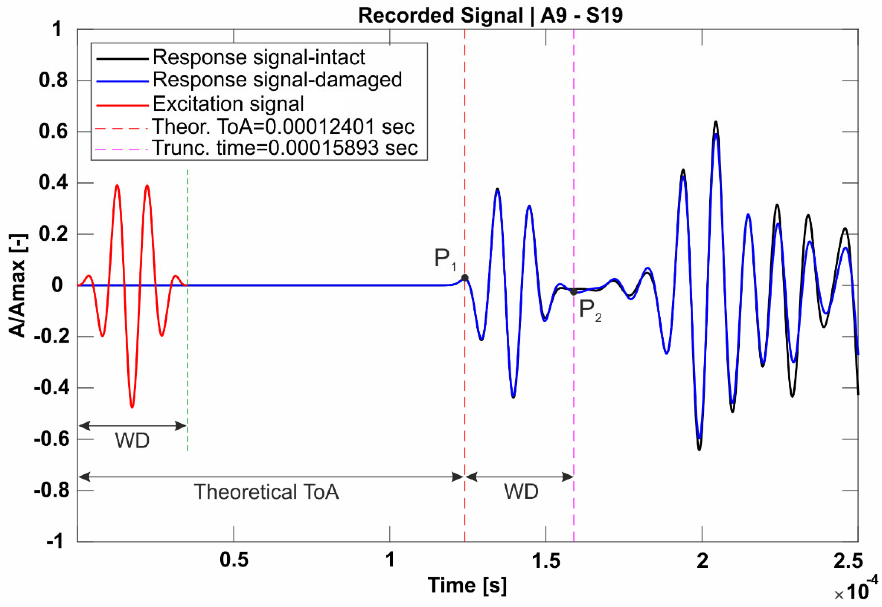
We incorporate the time-gating approach in one of our trials within this paper. In this method, the signal captured by a sensor is trimmed, commencing at a specific time point (P1) and concluding at another time point (P2) subsequent to the initiation.

Multiple time gates are explored in this study to determine the most optimal time duration for improved damage localization. The concept of time-gating is depicted in Figure 1 where the red line represents the excitation signal, with its duration indicated as WD. Following the acquisition of the theoretical ToA, point P1 is determined on the response signal, while point P2 is defined by adding WD to the theoretical ToA which is expressed by the duration from zero to the green dot line in Figure 1.

All attempts applied to the alpha interpolation method with the old numbering and iteration technique are performed considering the time gate between P1 and P2 as shown in Figure 1. Time gating is applied to signals of each AS path for both intact and damaged cases of the specimen.

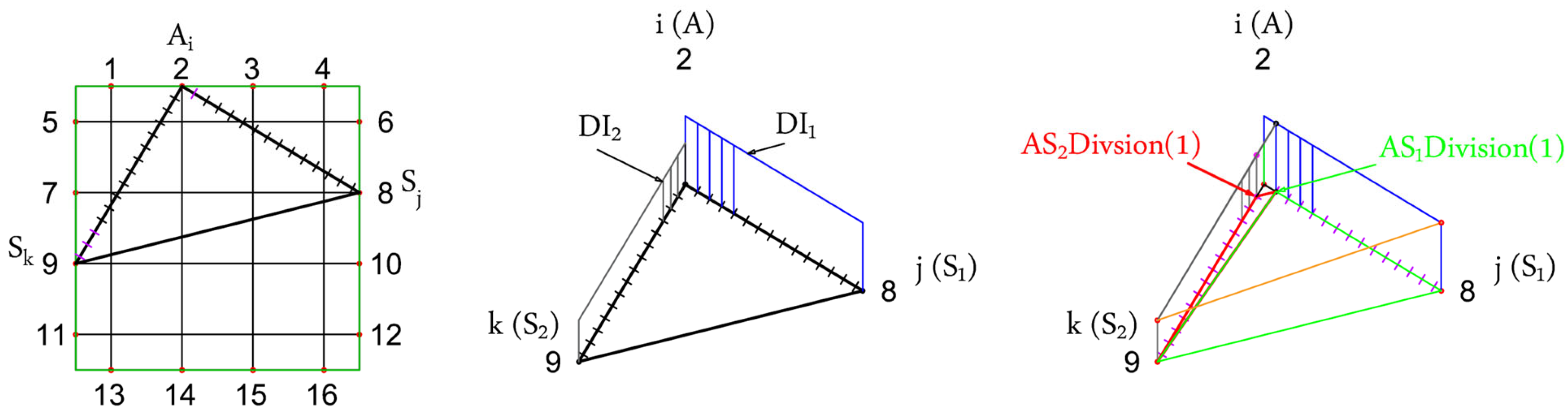
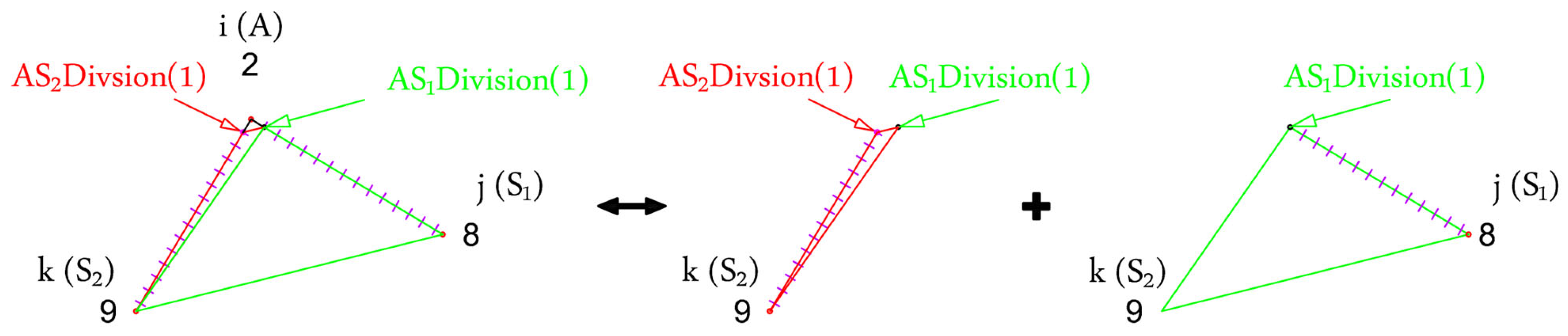
2.3. Recent Triangle Interpolation Method

In the previous publication of our group [4,14,18], we investigated damage detection using the triangular-based interpolation algorithm where two paths are considered at each time between one actuator and two other sensors attached to the surfaces of the specimen. However, this included an additional generation of two sub-triangles of the generated triangle to avoid assigning two values of the $DI$ value corresponding to the actuator point. This is shown in Figure 2 and Figure 3, where each of the original paths $A$-$S_1$ and $A$-$S_2$ are first divided into a certain number of divisions based on the predefined interpolation element size. Then the first point generated on each path is considered to create a new sub-triangle. Thus, we get two triangles from each triangle as shown in Figure 2 and Figure 3. The first triangle in red, while the second one is shown in green color.

2.4. Alpha Ratio Interpolation Methodology

The presented technique is implemented to get rid of the additional steps and data generation required within the method discussed in the previous section.

For the implementation of the alpha interpolation method, two AS paths are required including their $DI$ values. As illustrated in Figure 4, a reference point ($S_0$) is taken to acquire the reference angle (${\alpha }_0$) that defines the angle of the path $A$-$S_1$. Similarly, the path $A$-$S_2$ is defined using the angle ($\alpha$), defining its angle w.r.t. as the first path.

Thus, for a random point ($P_x$) within the angle $S_1$-$A$-$S_2$, the $DI$ can be calculated based on the linear relationship between each angle and its corresponding $DI$ value as follows

$$\frac{{\alpha }_0}{D{I}_1}=\frac{{\alpha }_0+{\alpha }_x}{D{I}_x}=\frac{{\alpha }_0+\alpha }{D{I}_2}$$

(9)

$$D{I}_x=D{I}_1+\frac{{\alpha }_x}{\alpha }\left(D{I}_2-D{I}_1\right)$$

(10)

where ${\alpha }_x$ is the angle between the A-$S_1$ path and the path between the actuator A and the random point $P_x$.

In our developed method, interpolation occurs for predefined seeds evenly distributed across the specimen. Seed generation is based on a preset interpolation mesh size within the specimen. This yields a fixed number of geometric data points instead of creating nodes within each interpolation triangle, as performed in the previous method [16]. Consequently, we explore two possible domain considerations for the interpolation process, elaborated in the following sections.

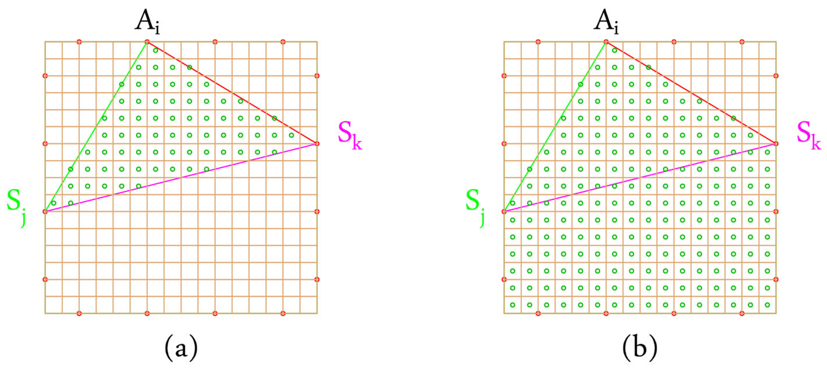
2.4.1. Triangles Interpolation for Damage Detection

In this interpolation domain picking strategy, the predefined seeds are solely considered if they fall within the boundary outlined by each pair of AS paths ($A$-$S_1$, $A$-$S_2$), forming a triangle A-$S_1$-$S_2$. This is illustrated in Figure 5a where only points within the generated triangle are considered.

2.4.2. Triples Interpolation for Damage Detection

In this interpolation domain picking strategy, the predefined seeds are exclusively considered if they fall within the region defined by the angle formed between the trio S₁-A-S₂. This approach assumes a uniform value of the $DI$ for all points sharing the same angle with the reference path. Figure 5b illustrates the region encompassed by this trio and showcases sample seeded points within this area.

2.5. The Impact of Averaging Interpolation Results on Damage Localization

In the context of the previous damage detection method, we observed certain approximation processes occurring. The resulting $DI$ values from various triangles, sharing the same geometrical location, were either accumulated or averaged. Consequently, further investigation was undertaken to compare both approaches.

However, in our modified method (alpha interpolation), employing the new numbering and iteration system, this loss of information is mitigated.

2.5.1. Accumulating DI of Interpolation Points

During the process of interpolating the $DI$ values within each seed node, many values at the same seed node might be acquired. Thus, these values are summed up for the corresponding node. Figure 6 illustrates this phenomenon, where at node (201), three values from three different triangles are summed up.

2.5.2. Averaging DI of Interpolation Points

In this policy, the $DI$ values of each seed node are averaged in the case of having multiple values at one node. This is also shown in Figure 6 where node (216) has four different values of $DI$ resulting from four different triangles. Thus, the final value of $DI$ at this node is the average of all these four values.

2.6. Recent vs. Modified Alpha Interpolation Methods

In addition to the previously mentioned alpha interpolation methodology (Section 2.4), a modified numbering protocol and iteration system is introduced in this research to get rid of the additional data generation and information loss. In

Table 1. Alpha modifications to the damage detection method.

Difference Aspect	Previous Damage Detection Method	Modified Alpha Interpolation Method
Numbering protocol	Starting from top-left and increase horizontally	Starting from top-left and increase clockwise
Signal processing (truncation)	All signals are truncated at the same moment (at specific value)	Each signal is truncated based on its theoretical ToA or its first detected peak
Iteration methodology	Starts from first PZT location, iterate on three loops on i, j, k for the actuator A, sensor S1, and sensor S2 respectively. The iteration is on all possible values where i, j, k are not allowed to take the same value	Starts iterating i from the first PZT location for A and iterates on j from i + 1 internally for S1, while the value of j + 1 is always taken for S2.

, a comparison between the previous strategy and the modified alpha interpolation method is summarized. Furthermore, an illustrative sketch of the main differences between both methods is presented in Figure 7.

The new numbering protocol is designed to iterate without overlap between the triangles generated from the AS paths. The iteration policy is adjusted accordingly to achieve this objective. In this method, the seed nodes acquire a single $DI$ value for each round of excitation. Consequently, the need to average or accumulate $DI$ values arises only between different excitation rounds.

As an explanation of the modified alpha interpolation method, on the right-hand side of Figure 7, the first iteration triangle is constructed from A2-S4-S5. In the next iteration, the triangle built of points A2-S5-S6 is considered for the $DI$ interpolation of each point inside its surface. In this manner, the iterations are carried out until all areas are covered by the PZTs except the blind areas on the corners. These areas can be also interpolated in the case of considering areas constructed by triples instead of triangles between AS paths. Both scenarios are thoroughly investigated in this paper.

3. Numerical Simulation

All trials applied in this paper are performed based on the numerical simulation of different models that correspond to the investigated cases. For each trial, two specimens of a 2D concrete plate are modeled as a linear elastic material with the dimensions of $0.4\times 0.4\times 0.04$ [m]. The only difference between the trials is the location and/or size of the hole for the damaged case models. One model is considered for the reference intact case, while the other model is implemented to refer to the damaged case.

The software used for the numerical simulation is ABAQUS/EXPLICIT R2018x. After the simulation is performed, the acquired response signals are processed based on the Alpha ratio interpolation method. This results in damage detection and localization within the specimen. The post-processing of the signals and the interpolation steps are applied using a group of MATLAB R2022b codes developed for this purpose.

3.1. Models’ Inputs and Characteristics

3.1.1. The Material Properties

The material of all simulated models is assumed to be linear concrete, with the material properties summarized in

Table 2. Material properties of concrete.

Young’s modulus [GPa]	30
Poisson’s ratio	0.1
Density [kg/m3]	2400
$\alpha$ (damping coefficient)	2058.23
$\beta$ (damping coefficient)	1.105 $\times {10}^{-8}$

.

The Rayleigh damping coefficients α and β are chosen based on literature recommendations [18], particularly from studies utilizing the direct pitch-catch model, a widely employed method in non-destructive testing for material and structural assessment. Tian et al. extensively detailed the process of calculating these damping coefficients in their research [19].

3.1.2. Applied Excitation Signal and Boundary Conditions

The excitation signal considered for all trials is applied as an external force. The signal function is considered a 3.5-cycle Hanning-windowed tone burst:

$$P_{\left(t\right)}=\left\{\begin{array}{cc}\left[1-cos\left(\frac{2\pi }{N}t\right)\right]sin\left(2\pi ft\right),\hfill & \mathrm{for}\hspace{1em}\hspace{1em}0\le t\le \frac{N}{f}\hfill \\ \hspace{1em}0 ,\hfill & \mathrm{for}\hspace{1em}\hspace{1em}\hspace{1em}t>\frac{N}{f}\hfill \end{array}\right.$$

(11)

where

f is the signal frequency (in the model 100 kHz).

N is the number of cycles (in the model 3.5 cycles).

T is the time (duration of the signal) (in the model 3.5 × ${10}^{-5}$ s).

$P_{\left(t\right)}$ is the excitation by the actuator.

A high frequency of 100 kHz is selected for its capability to detect small defects in the concrete structure and its effectiveness in minimizing ambient noise that could otherwise interfere with defect detection. This choice facilitates the isolation and analysis of signals from the concrete specimen. The ABAQUS/EXPLICIT package was used to perform the analysis, employing C3D8R eight-node prismatic finite elements with reduced integration and Hourglass control.

The boundary conditions are established through four supporting points located at the bottom corners of the specimen. An additional condition is defined at the opposite two corners to the side where the excitation occurs. The boundary conditions are illustrated in Figure 8. It is noteworthy that the second set of conditions, associated with the excitation point, is specified for each side of the excitation to align with the respective direction. This approach aims to prevent specimen movement in the excitation direction, especially when high amplitudes are applied.

3.2. Investigated Cases

In this section, three main aspects are presented for the importance of the damage localization within a given specimen. Firstly, different damage locations and sizes are implemented. Secondly, the field of interest within the interpolation process is investigated. Lastly, an example of the enhanced method of alpha interpolation methodology with the modified iteration technique is presented. It is noteworthy that the actual hole location is depicted as a black circle in all of the following figures.

3.2.1. Different Damage Locations and Sizes

In this endeavor, damage localization is performed using the alpha interpolation method alongside the previous numbering and iteration strategy. Furthermore, the $DI$ matrix for each case is derived from gated signals between their theoretical ToF and ToF + WD. A summary of all experimented cases is presented in

Table 3. Investigated cases for the alpha interpolation method with old numbering and iteration policy.

Investigated Case	Trial ID	xc	yc	rc
Different locations of the hole	1-1	0.12	0.32	0.02
	1-2	0.28	0.12	0.02
	1-3	0.15	0.10	0.02
Different size of the hole	2-1	0.12	0.32	0.01
	2-2	0.28	0.12	0.005
	2-3	0.15	0.10	0.015

, where xc, yc, and rc are coordinates and the radius of the implemented hole. The number of PZTs used in this attempt is 16, while the geometry is as defined in the previous section.

It is important to note that the AS paths situated along the edges of the specimen are disregarded due to their adverse impact on our method. They introduce misleading information to the $DI$ values and consequently affect the accuracy of damage localization. In the results chapter, an illustrative example of the detrimental effect caused by AS paths located at the boundary is presented, as seen in Figure 9.

Additionally, all the results presented in this attempt are acquired by averaging all the values of $DI$ for each seed node within the specimen between all excitation cases and all generated triangles within each excitation case.

3.2.2. Comparison between Triple and Triangle DI Interpolation

This comparison aims to derive meaningful conclusions regarding the distinct effects when considering only seed points within triples formed from AS paths and interpolating points solely within the triangles formed by those AS paths. The algorithm utilized for this comparison is alpha interpolation with the old numbering protocol and iteration technique. Additionally, the influence of averaging and accumulating for $DI$ during the interpolation is examined for each trial.

3.2.3. Improvements on the Alpha Algorithm

As the alpha interpolation method was initially developed based on a previous damage localization method, several aspects of the algorithm required modification. This involved adjusting the numbering protocols of PZTs and the corresponding iteration technique to minimize information loss during the $DI$ interpolation process. Additionally, the signals considered for energy calculation were examined to enhance damage localization.

As mentioned in Section 2.6, the new iterating system aims to cover the maximum space of the specimen with one actuator and all other sensors, avoiding data accumulation for points included in different triples or triangles. To explore this, similar trials with the improved algorithm are implemented: one considering the seed points within formulated triples and the second considering seed points within triangles formulated from each pair of AS paths.

In the tuning process of signal truncation, only one geometrical variant is considered (trial 1-3). In this context, the signal of each AS path is processed with one of four truncation policies. The first truncation policy involves truncating the signal at the time corresponding to its first detected peak. Another truncation policy is defined at the first detected peak plus half of the excitation wave duration. The other two truncation trials are similar to the first and second trials, with one key difference: the truncation point depends on the theoretical ToA instead of the first detected peak of the signal.

4. Results

In this section, all the simulation results are presented. Firstly, the alpha interpolation method with previous numbering and iteration techniques is tested with specimens of different locations and sizes of the damage to inspect its sensibility in the damage localization. After that, a comparison using the same method is applied between the case of considering the enclosed area of the specimen within each triple generated from the AS paths and the case of considering only the region defined by the triangle formed from each two AS paths with the same actuator. Lastly, further improvement strategies are presented, which include a similar comparison example to the previous one but adapt the new numbering protocol and iteration strategy. The second improvement strategy is covered by several truncation examples of the response signals before applying the modified alpha interpolation method for damage localization.

All models presented in the following sub-sections have the same time increment ($2.8\times {10}^{-8}$ s) and a mesh size of (0.00105 m) that satisfies the critical conditions of the time increment and mesh size presented in [20]. Furthermore, the element length used for the interpolation part is considered to be equal to (0.004 m) to provide convenient visualization of the detected damaged area.

4.1. Different Damage Locations and Sizes

In these simulations, the alpha interpolation method with the previous numbering and iteration strategy is implemented. As mentioned in Section 3.2.1, the time-gating approach is applied for processing the acquired response signals. The gating domain starts at the theoretical ToA and ends at the duration of ToA + WD. Furthermore, all trials in this chapter involve averaging the $DI$ values between each generated triple and also between each excitation point.

4.1.1. Different Damage Location

Three locations are chosen to ensure that the damage is asymmetric and does not align with any symmetric axis of the specimen where the radius of all three trials is 0.02 m, as seen in Table 3.

In Figure 9, the results of trial (1-1) are presented, showcasing damage localization by considering all AS paths between the PZTs on the left-hand side. On the right-hand side, the case of neglecting AS paths located on the edges of the specimen is shown. Black dots indicate the location of each PZT. The values in subsequent figures represent the $DI$ values after interpolation between all paths considered for each case.

Additional trials, (1-2) and (1-3), are performed similarly, and the resulting damage detection is presented in Figure 10 and Figure 11, respectively. In trial (1-2), the effect of the boundary AS paths is not very noticeable since the damage is located far from the boundaries. However, trial (1-3) exhibits the same misleading effect.

AS paths located on the boundary of the specimen lead to misleading information on the damage location. Thus, it is advisable to neglect them during the Damage detection process.

4.1.2. Different Damage Size

The same locations considered for the previous trials are adopted in the following trials, but the diameter of the hole is varied to gain insight into the method’s sensitivity to the damage size. The radius of the hole for each trial is assigned as mentioned in Table 3.

In Figure 12, trial 2-1 presents the interpolated $DI$ values, which lead to damage localization. However, it is worth noting that the actuator located on the edges near the hole is largely affected by the damaged area and how close is it to the edge, as seen in Figure 12a.

Additionally, considering an even smaller radius for the hole, in trial (2-2), the damage is still spotted with a smaller surrounding area than the similar case in trial (1-2), see Figure 13a. However, the misleading values resulting from boundary AS paths still appear in trial (2-3) even when the hole is small, as seen in Figure 14a.

By comparing the cases in Figure 9a and Figure 12a, we can conclude that there is a linear relationship between the size of the damage and the value of the misleading $DI$ generated by the boundary AS paths. However, the detected area around the damage does not lead to accurate localization of the damage. Thus, further investigation and improvement are applied to the alpha interpolation method in the following chapters.

4.2. Interpolation Regions and Assessing the Impact of DI Value Averaging

In this chapter, we investigate the area considered for each interpolation, focusing on two cases as mentioned in Section 2.5. Additionally, we internally inspect the effect of averaging the $DI$ values for each of these cases, as described in Section 2.6.

4.2.1. Interpolation in Triples

In this trial, the area enclosed within each A-S₁-S₂ triple is considered for $DI$ interpolation. This assumes that all points located on each array starting from A and situated between S₁ and S₂ have the same $DI$ value, which is linearly interpolated between DI1 and DI2.

Trial (1-3) is selected for this investigation with signal time-gating applied between each signal’s theoretical ToA and the time corresponding to ToA + WD. Additionally, $DI$ values are not averaged between each triple and each excitation case. Furthermore, the number of PZTs is increased to 20 to obtain better damage localization. Since the previous investigation revealed that AS paths provide misleading information, they will be neglected in all further attempts.

In Figure 15, the resulting damage detection is presented. The left-hand side visualizes the interpolated $DI$, while the right-hand side shows only the points with the top 10% of the $DI$ values within the specimen. This approach is applied because our goal is to identify the maximum value of $DI$, considered the center of the detected damage.

To gain insight into the impact of averaging $DI$ interpolated values on damage localization, the case presented in Figure 16 is examined. Here, it can be observed that the averaging process contributes to reducing the misleading content of the $DI$ values.

Comparing Figure 15 and Figure 16, we notice that the detected damaged area is reduced and fits the real existing hole better.

4.2.2. Interpolation in Triangles

Similar to the investigation in the previous section, trial (1-3) is considered. The only difference is that we limit our consideration to nodes within the area defined by Actuator A and the other two sensors, S₁ and S₂, for $DI$ value interpolation.

In Figure 17, the interpolated $DI$ values are not averaged between each constructed triangle; rather, all $DI$ values are accumulated. However, the detected damaged area is slightly shifted from the center of the actual damage, resulting in inaccurate damage localization.

On the other hand, Figure 18 presents damage localization with the averaging of interpolated $DI$ values between each $A$-$S_1$-$S_2$ triangle. This leads to improved localization of the damage by considering the top 10% of $DI$ values, as shown on the right-hand side of the figure.

Comparing Figure 16 and Figure 18, we conclude that averaging the interpolated $DI$ values within triangle areas results in better localization of the $DI$. However, there is still confusion regarding the detected area, where the area between the damage and the nearest PZTs exhibits high values of $DI$ compared to the area located within the real damage location.

4.3. Improvement of the Alpha Interpolation Method

As mentioned in Section 3.2.3, two main improvements are applied to the alpha interpolation method. Both enhancements will be discussed in the following sections. The implementation occurs on two levels. The first level involves reducing the averaging processes by avoiding intersections between constructed triangles.

The modified numbering protocol is designed to correspond to the iteration technique, where each iteration applies $DI$ interpolation to all seed nodes included within a triangle. Each iteration covers one part of the specimen in 2D. Thus, at the end of all iterations, all nodes are linearly interpolated corresponding to their bounding AS pairs, as described in Section 2.6.

The second level involves the preprocessing step applied to the simulation response signals. This modification is motivated by the fact that the energy change we are trying to capture depends on how much content of the signals is considered for its calculation. Although previous attempts used a time gate between the theoretical ToA and the time corresponding to ToA + WD, some of the response signals experience reflections from the edges, which may occur after two-thirds of the first arriving wavelet. These reflections can affect the quality of the considered signal. In this context, four signal truncation possibilities are considered, as presented in

Table 4. Truncation policies for the enhanced alpha interpolation method.

Trial Nr.	Start of Truncation [s]	End of Truncation [s]
1	0	First detected peak
2	0	First detected peak + W/2
3	0	Theoretical ToA
4	0	Theoretical ToA + WD/2

.

In the first trial, the first detected peak in signals of each AS path is considered the truncation end. Thus, we only obtain a useful part of the signal including the first start of the arriving signals at each sensor. This is clearly noticeable in Figure 19, where the detected damage area is identical to the real damage location.

Adding half of the excitation signal duration to the truncated part of each response signal also gives good localization of the damage but also shows some distribution due to the arrival of reflected waves to the sensors of some AS paths, as seen in Figure 20.

On the other hand, considering the theoretical ToA as the truncation point of the signal results in a more accurate localization of the damage as shown in Figure 21. Furthermore, when considering only the top 10% of the $DI$ values after the interpolation, we obtain a perfect match to the real damage size as shown on the right-hand side of Figure 21.

By adding half of the excitation signal duration to the truncation segment, we still obtain a good detection of the damage as shown in Figure 22. However, without considering the top 10% of $DI$ values, the determination of the damage size is not accurate. Furthermore, a small shift of the damage center takes place due to the arrival of small reflections within some AS paths.

5. Conclusions and Recommendations

The application of the modified alpha interpolation method guarantees suitable damage localization. However, it is important for the utilization of this method to choose a suitable truncation point of the arrival signal at each signal. The modifications added to the recent interpolation method, used in [14,16], add more accuracy to the damage detection in 2D due to the minimization of the number of approximations within the interpolation of the $DI$ value for each point within the specimen.

The developed method requires having a reference state of the inspected specimen. However, good damage localization depends strictly on the quality of the considered signals for the calculation of the $DI$ and is extremely sensitive to any reflected signals other than the direct signal between each actuator and sensor. Thus, it is advisable to obtain a close look at the response signals for different AS paths for both reference and inspected cases to determine the critical point of the truncation segment.

The method has not yet been evaluated for the detection of multiple damaged points within one space. Thus, it is recommended to investigate further regarding this case. However, one workaround is by dividing the space into sub-domains and dealing with each sub-domain as one block surrounded by a set of PZTs, which work together to determine the damage existence within that sub-domain.

References

1. Das Adhikari, M.; Kim, T.-H.; Yum, S.-G.; Kim, J.-Y. Damage Detection and Monitoring of a Concrete Structure Using 3D Laser Scanning. Eng. Proc. 2023, 36, 1. [Google Scholar] [CrossRef]
2. Campeiro, L.M.; da Silveira, R.Z.M.; Baptista, F.G. Impedance-based damage detection under noise and vibration effects. Struct Health Monit. 2018, 17, 654–667. [Google Scholar] [CrossRef]
3. Diab, A.; Nestorović, T. Convergence Study on Wave Propagation in a Concrete Beam. In Proceedings of the 11th International Workshop NDT in Progress, Prague, Czech Republic, 4–7 October 2021. [Google Scholar]
4. Diab, A.; Nestorović, T. Damage Index Implementation for Structural Health Monitoring. In Recent Trends in Wave Mechanics and Vibrations. WMVC 2022; Dimitrovová, Z., Biswas, P., Gonçalves, R., Silva, T., Eds.; Springer: Cham, Switzerland, 2023; pp. 783–791. [Google Scholar] [CrossRef]
5. Doghri, W.; Saddoud, A.; Fourati, L. Sensor Placement Strategy for SHM: Application of the Great Mosque of Sfax. In Proceedings of the International Conference on Advanced Information Networking and Applications, Sydney, Australia, 13–15 April 2022; Springer International Publishing: Cham, Switzerland, 2022; pp. 238–248. [Google Scholar] [CrossRef]
6. Goyal, D.; Pabla, B.S. The Vibration Monitoring Methods and Signal Processing Techniques for Structural Health Monitoring: A Review. Arch Comput. Methods Eng. 2016, 23, 585–594. [Google Scholar] [CrossRef]
7. Huang, J.Q. Non-destructive evaluation (NDE) of composites: Acoustic emission (AE). In Non-Destructive Evaluation (NDE) of Polymer Matrix Composites; Woodhead Publishing: Sawston, UK, 2013; pp. 12–32. [Google Scholar] [CrossRef]
8. Jiang, S.; Cheng, Y.; Zhang, J. Vision-guided unmanned aerial system for rapid multiple-type damage detection and localization. Struct. Health Monit. 2023, 22, 319–337. [Google Scholar] [CrossRef]
9. Kafle, B.; Zhang, L.; Mendis, P.; Herath, N.; Maizuar, M.; Duffield, C.; Thompson, R.G. Monitoring the Dynamic Behavior of The Merlynston Creek Bridge Using Interferometric Radar Sensors and Finite Element Modeling. Int. J. Appl. Mech. 2017, 9, 1750003. [Google Scholar] [CrossRef]
10. Kallas, J.; Napolitano, R. Automated large-scale damage detection on historic buildings in post-disaster areas using image segmentation. Int. Arch. Photogramm. Remote Sens. Spat. Inf. Sci. 2023, 48, 797–804. [Google Scholar] [CrossRef]
11. Knitter-Piatkowska, A.; Guminiak, M.; Przychodzki, M. Application of discrete wavelet transformation to defect detection in truss structures with rigidly connected bars. Eng. Trans. 2016, 64, 157–170. [Google Scholar]
12. Koszewnik, A.; Lesniewski, K.; Pakrashi, V. Numerical Analysis and Experimental Verification of Damage Identification Metrics for Smart Beam with MFC Elements to Support Structural Health Monitoring. Sensors 2021, 21, 6796. [Google Scholar] [CrossRef] [PubMed]
13. Limongelli, M.P.; Manoach, E.; Quqa, S.; Giordano, P.F.; Bhowmik, B.; Pakrashi, V.; Cigada, A. Vibration Response-Based Damage Detection. In Structural Health Monitoring Damage Detection Systems for Aerospace; Springer Nature: Berlin/Heidelberg, Germany, 2021; pp. 133–173. [Google Scholar] [CrossRef]
14. Marković, N.; Nestorović, T.; Stojić, D.; Marjanović, M.; Stojković, N. Hybrid approach for two dimensional damage localization using piezoelectric smart aggregates. Mech. Res. Commun. 2017, 85, 69–75. [Google Scholar] [CrossRef]
15. Nasim Khan Raja, B.; Miramini, S.; Duffield, C.; Chen, S.; Zhang, L. A Simplified Methodology for Condition Assessment of Bridge Bearings Using Vibration Based Structural Health Monitoring Techniques. Int. J. Struct. Stab. Dyn. 2021, 21, 2150133. [Google Scholar] [CrossRef]
16. Nerlikar, V.; Mesnil, O.; Miorelli, R.; D’Almeida, O. Damage detection with ultrasonic guided waves using machine learning and aggregated baselines. Struct. Health Monit. 2024, 23, 443–462. [Google Scholar] [CrossRef]
17. Nestorović, T.; Diab, A. Wave propagation based damage detection in structural elements for civil engineering structures. In Proceedings of the 10th ECCOMAS Thematic Conference on Smart Structures and Materials, Patras, Greece, 3–5 July 2023; Saravanos, D.A., Benjeddou, A., Chrysochoidis, T., Theodosiou, T., Eds.; Department of Mechanical Engineering & Aeronautics University of Patras: Patras, Greece, 2023; pp. 999–1005. [Google Scholar] [CrossRef]
18. Stojić, D.; Nestorović, T.; Marković, N.; Marjanović, M. Experimental and numerical research on damage localization in plate-like concrete structures using hybrid approach. Struct. Control Health Monit. 2018, 25, e2214. [Google Scholar] [CrossRef]
19. Tian, Z.; Huo, L.; Gao, W.; Li, H.; Song, G. Modeling of the attenuation of stress waves in concrete based on the Rayleigh damping model using time-reversal and PZT transducers. Smart Mater. Struct. 2017, 26, 105030. [Google Scholar] [CrossRef]
20. Wah, W.S.L.; Chen, Y.-T. A new approach toward damage localization and quantification of structures under changing temperature condition. J. Low Freq. Noise Vib. Act. Control 2020, 39, 572–587. [Google Scholar] [CrossRef]
Figure 1. Excitation signal and response with the gated domain between points P1 and P2.
Actuators 13 00128 g001
Figure 2. Sub-triangulation for the D I interpolation.
Actuators 13 00128 g002
Figure 3. The two generated sub-triangles of A-S1-S2 triangle for D I interpolation.
Actuators 13 00128 g003
Figure 4. Alpha interpolation methodology.
Actuators 13 00128 g004
Figure 5. Comparison of triangular and triple domains for D I interpolation. (a) Triangle domains used for interpolation. (b) Triples considered as domains for interpolation. Green circles represent the considered seeds, and red circles indicate the positions of Actuators/Sensors.
Actuators 13 00128 g005
Figure 6. Averaging and accumulating D I values for damage detections.
Actuators 13 00128 g006
Figure 7. Comparison between generated triangles in (a) the recent damage detection method and (b) the modified alpha interpolation method. Interpolating for the excitation case at Ai = 2.
Actuators 13 00128 g007
Figure 8. Applied boundary conditions in the numerical simulation. Conditions in red are permanent, while conditions in blue are excitation direction-dependent.
Actuators 13 00128 g008
Figure 9. Damage localization using alpha interpolation (old iteration technique)—trial 1-1.
Actuators 13 00128 g009
Figure 10. Damage localization using alpha interpolation (old iteration technique)—trial 1-2.
Actuators 13 00128 g010
Figure 11. Damage localization using alpha interpolation (old iteration technique)—trial 1-3.
Actuators 13 00128 g011
Figure 12. Damage localization using alpha interpolation (old iteration technique)—trial 2-1.
Actuators 13 00128 g012
Figure 13. Damage localization using alpha interpolation (old iteration technique)—trial 2-2.
Actuators 13 00128 g013
Figure 14. Damage localization using alpha interpolation (old iteration technique)—trial 2-3.
Actuators 13 00128 g014
Figure 15. Damage localization with triple areas and without averaging D I —trial 1-3.
Actuators 13 00128 g015
Figure 16. Damage localization with triple areas and with averaging D I —trial 1-3.
Actuators 13 00128 g016
Figure 17. Damage localization with triangle areas and without averaging D I —trial 1-3.
Actuators 13 00128 g017
Figure 18. Damage localization with triangle areas and with averaging D I —trial 1-3.
Actuators 13 00128 g018
Figure 19. Damage localization using modified alpha interpolation with signal truncation at first peak.
Actuators 13 00128 g019
Figure 20. Damage localization using modified alpha interpolation with signal truncation at first peak + half of WD.
Actuators 13 00128 g020
Figure 21. Damage localization using modified alpha interpolation with signal truncation at theoretical ToA.
Actuators 13 00128 g021
Figure 22. Damage localization using modified alpha interpolation with signal truncation at theoretical ToA + half WD.
Actuators 13 00128 g022