
Comparison of Separation Control Mechanisms for Synthetic Jet and Plasma Actuators

Abstract
:1. Introduction
2. Problem Specifications
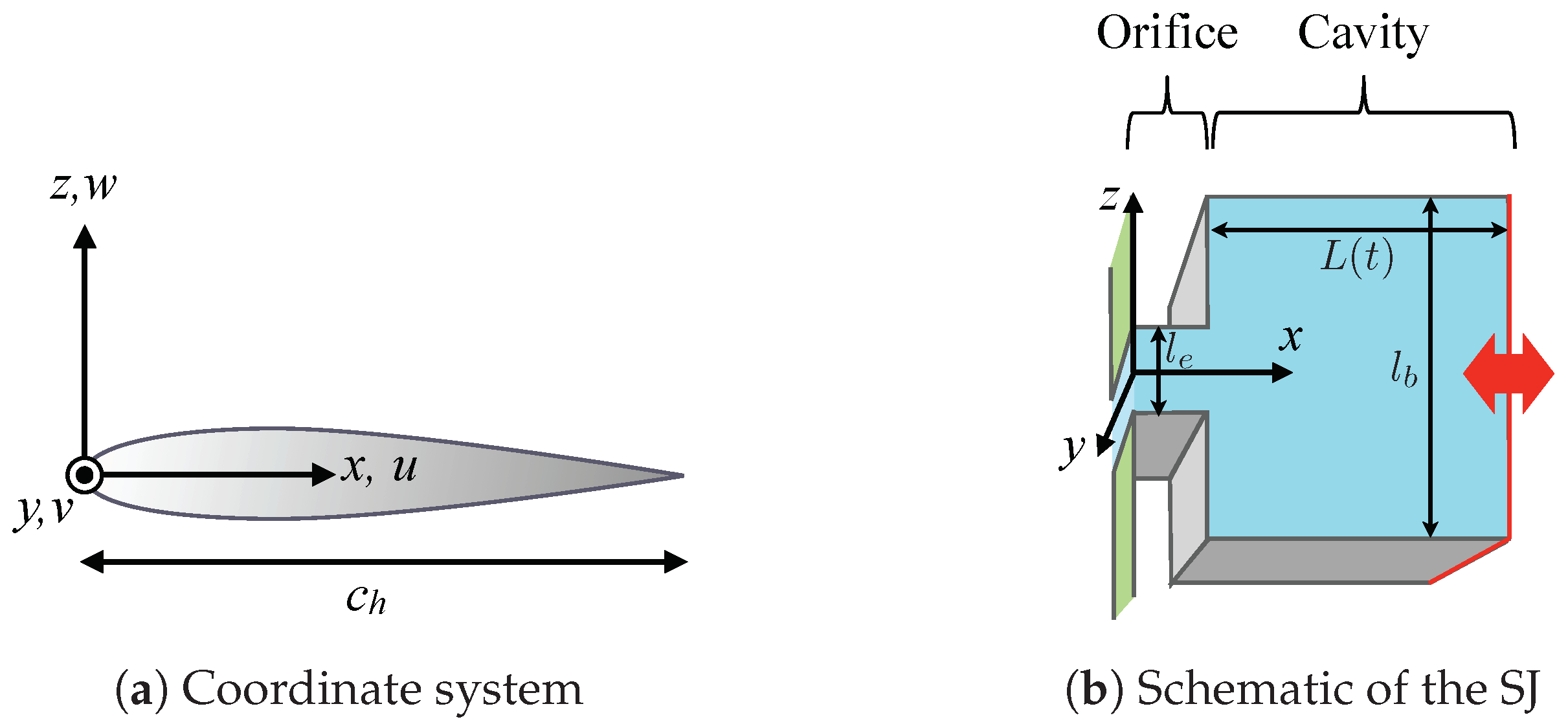
2.1. Separated Flow
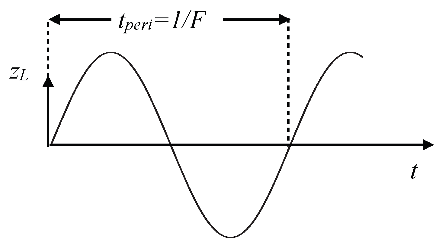
2.2. Configuration of the SJ

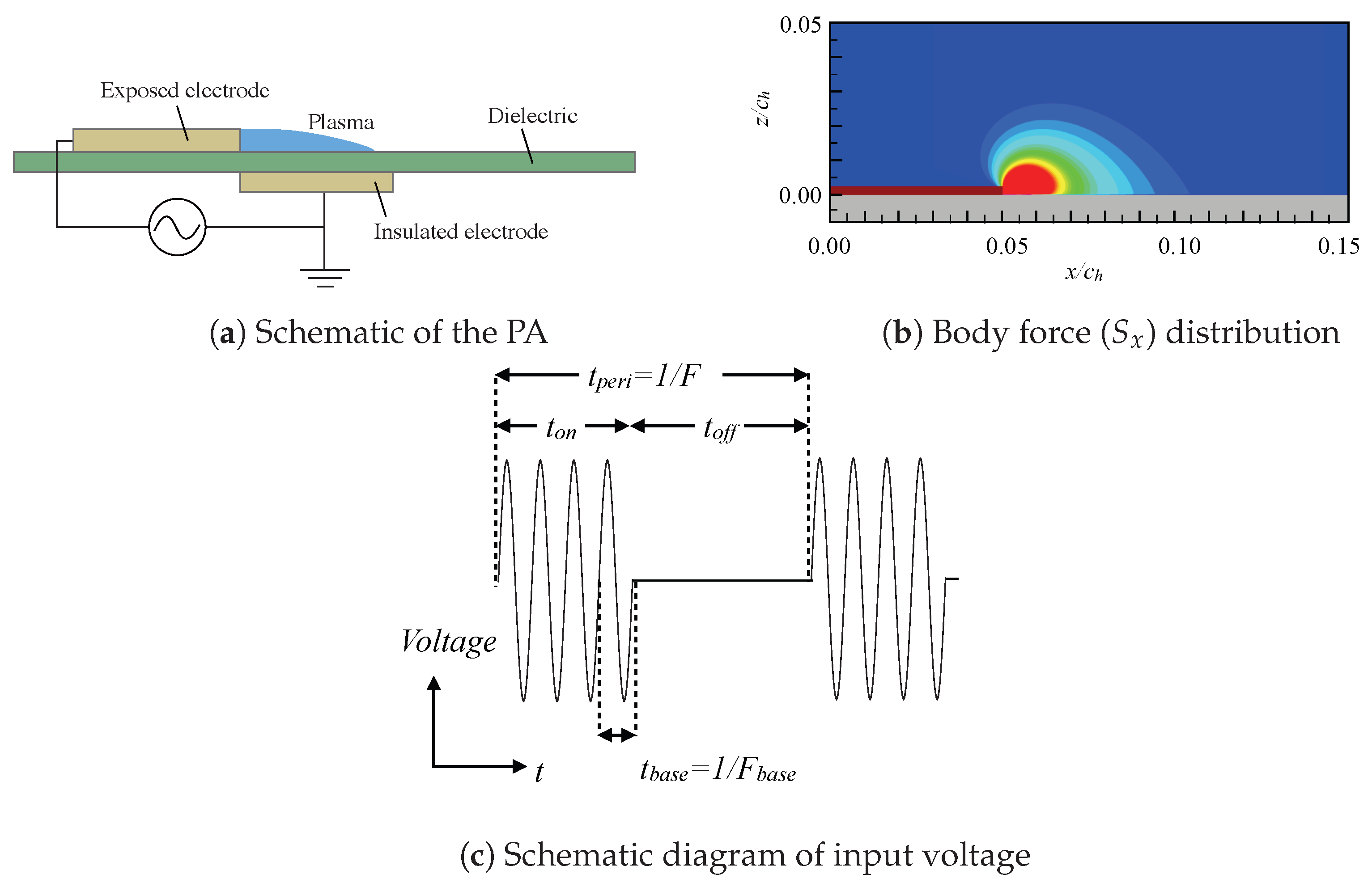
2.3. Configuration of the PA

2.4. Case Description
3. Methodology
3.1. Flow Solver
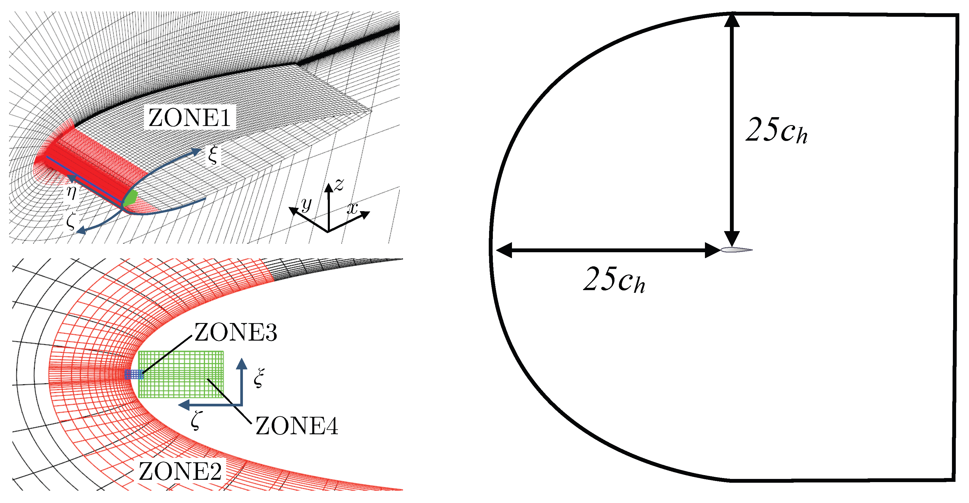
3.2. Computational Grids and Boundary Conditions
3.3. Validation and Verification
4. Results and Discussion
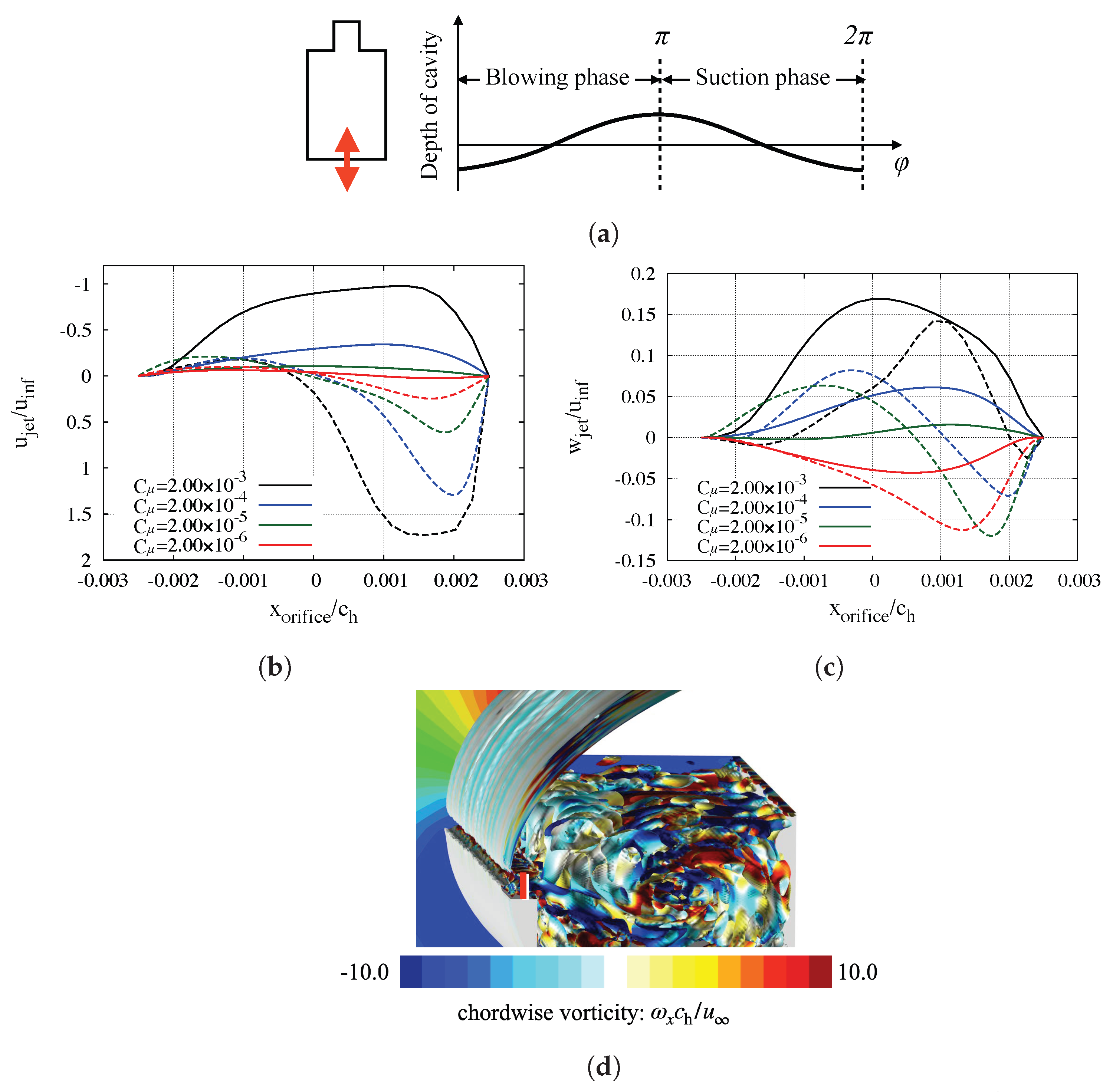
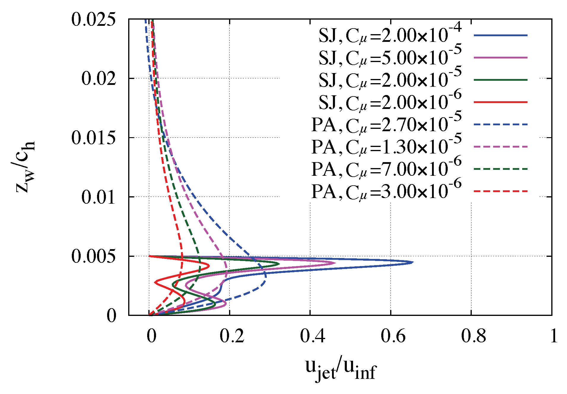
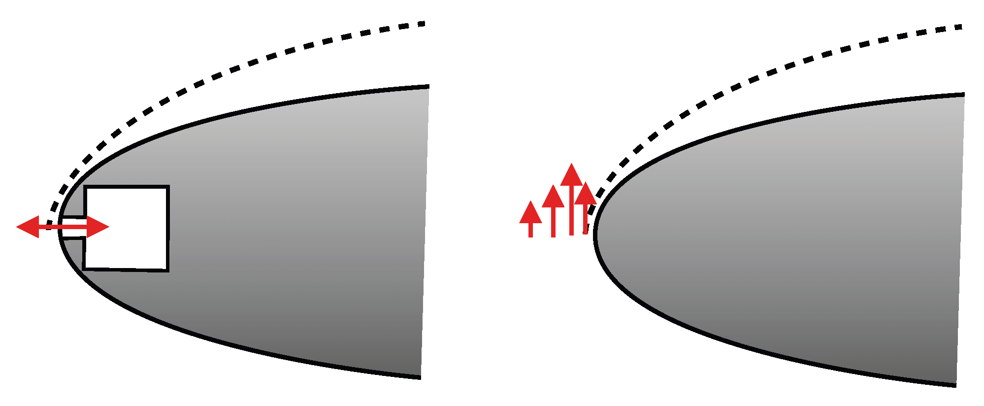
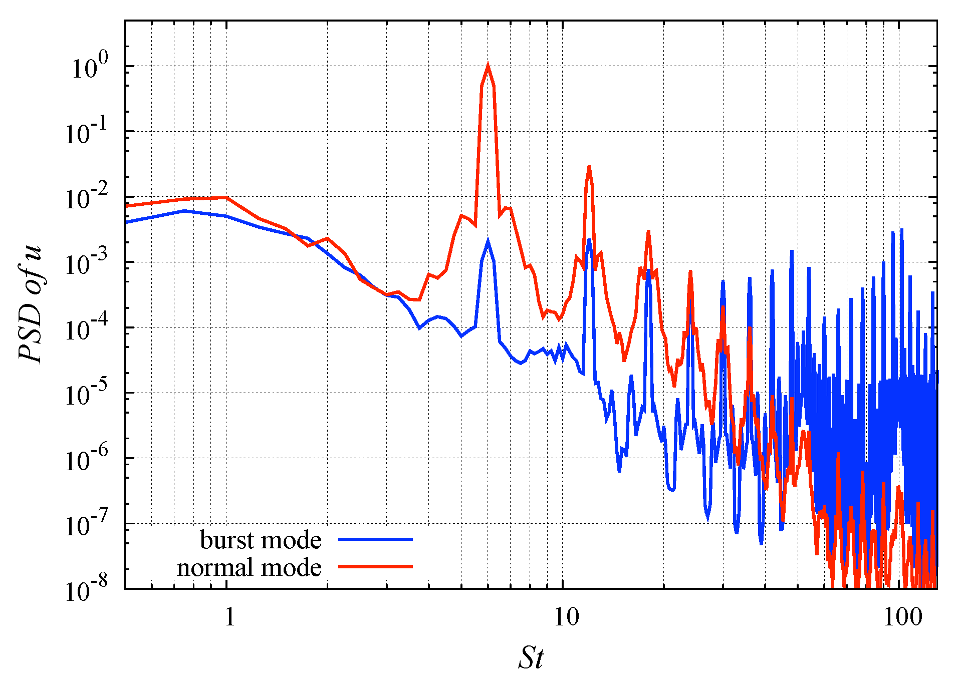
4.1. Differences of Induced Flows from the SJ and the PA
- A.
- Wall-tangential velocity;
- B.
- Three-dimensional flow structures;
- C.
- Spatial locality;
- D.
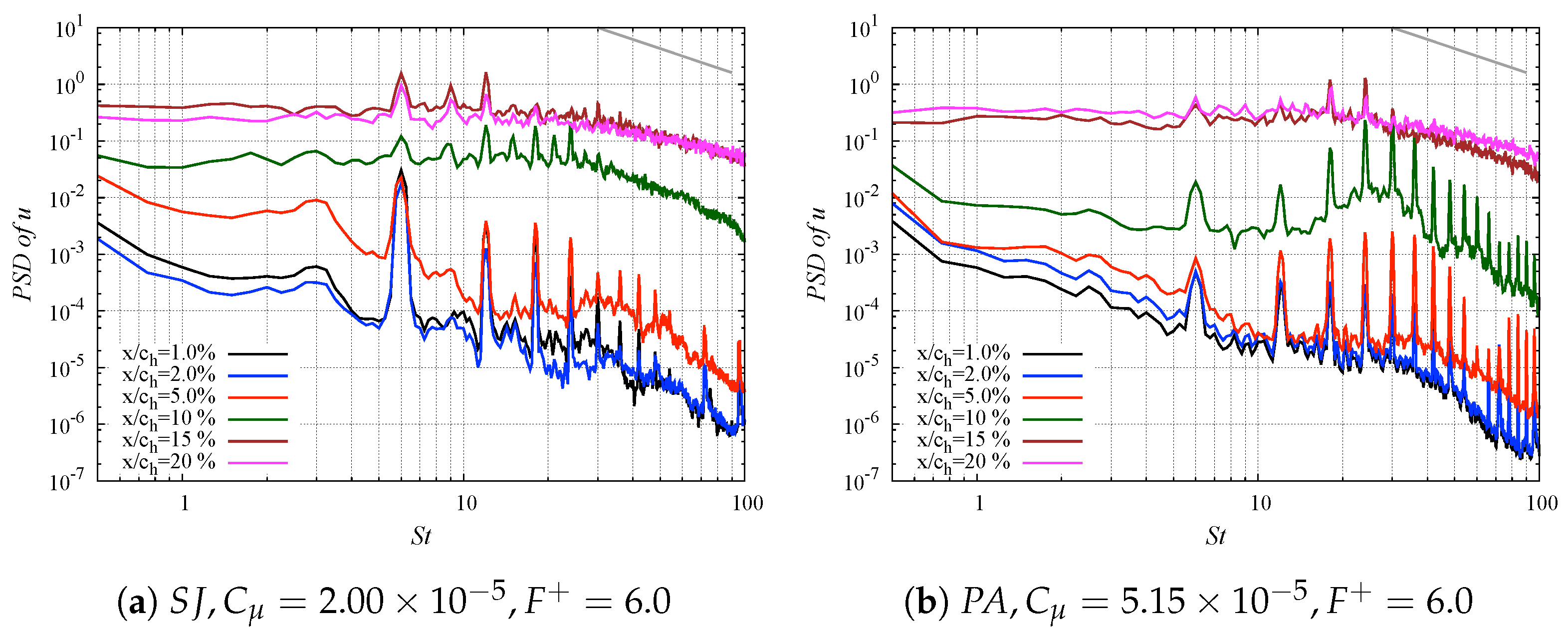
- Temporal fluctuation.
- A.
- Wall-Tangential Velocity

- B.
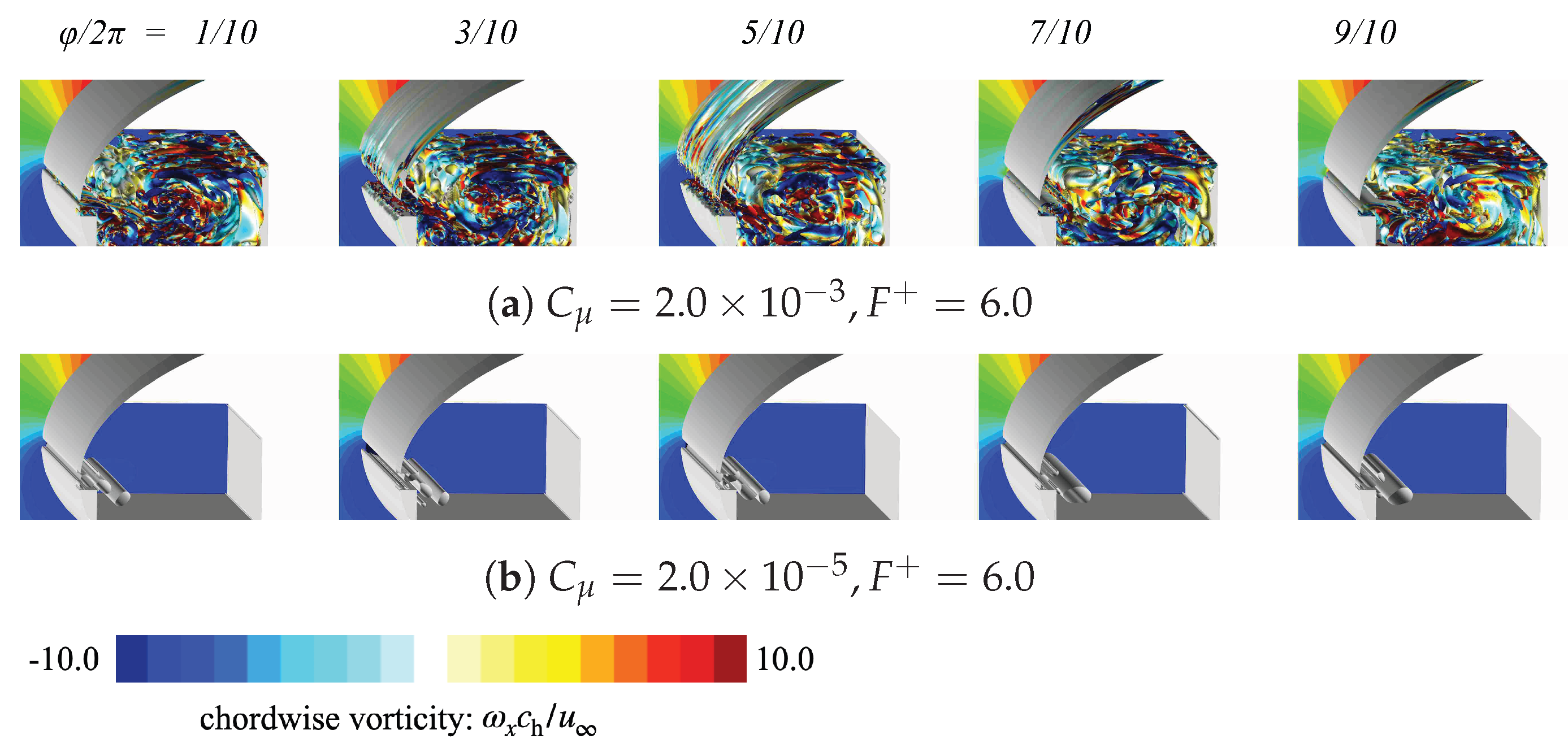
- Three-Dimensional Flow Structures


- C.
- Spatial Locality


- D.
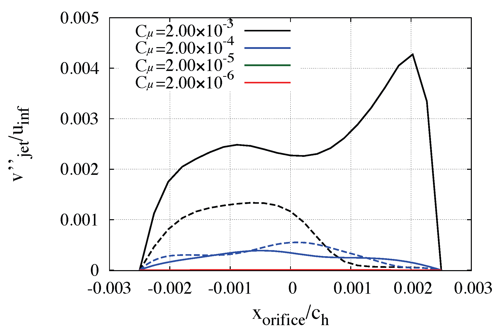
- Temporal Fluctuation

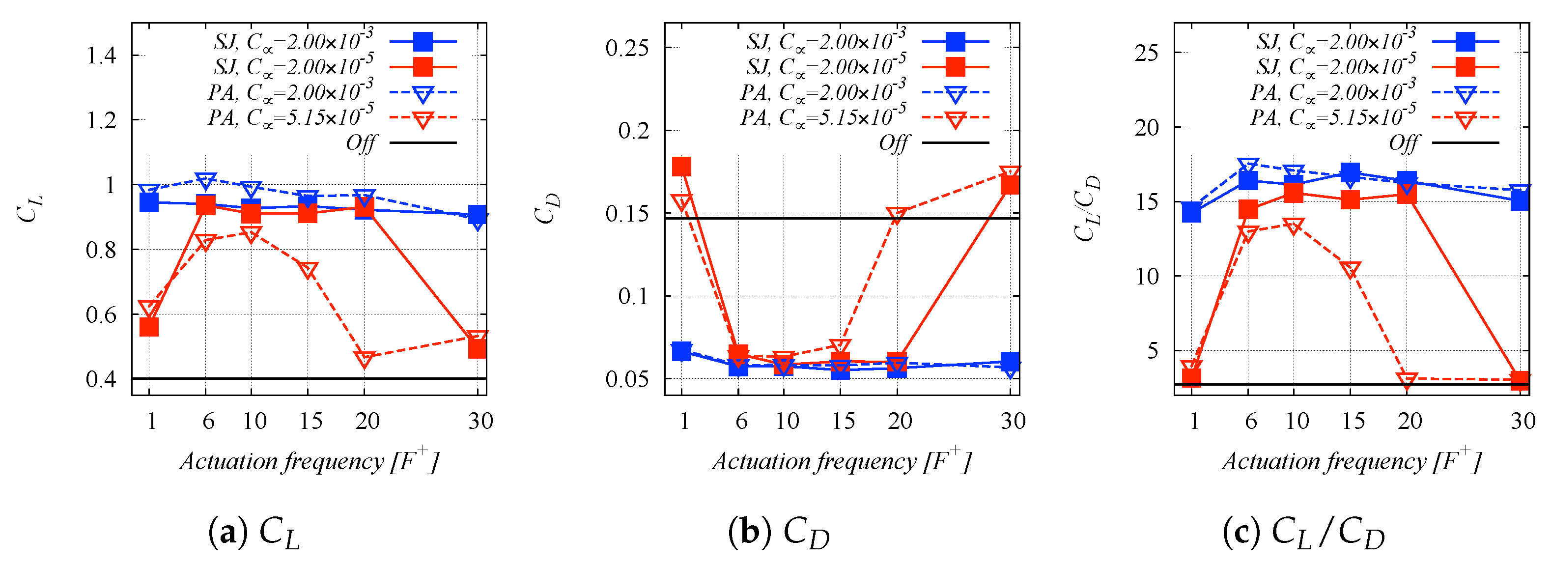
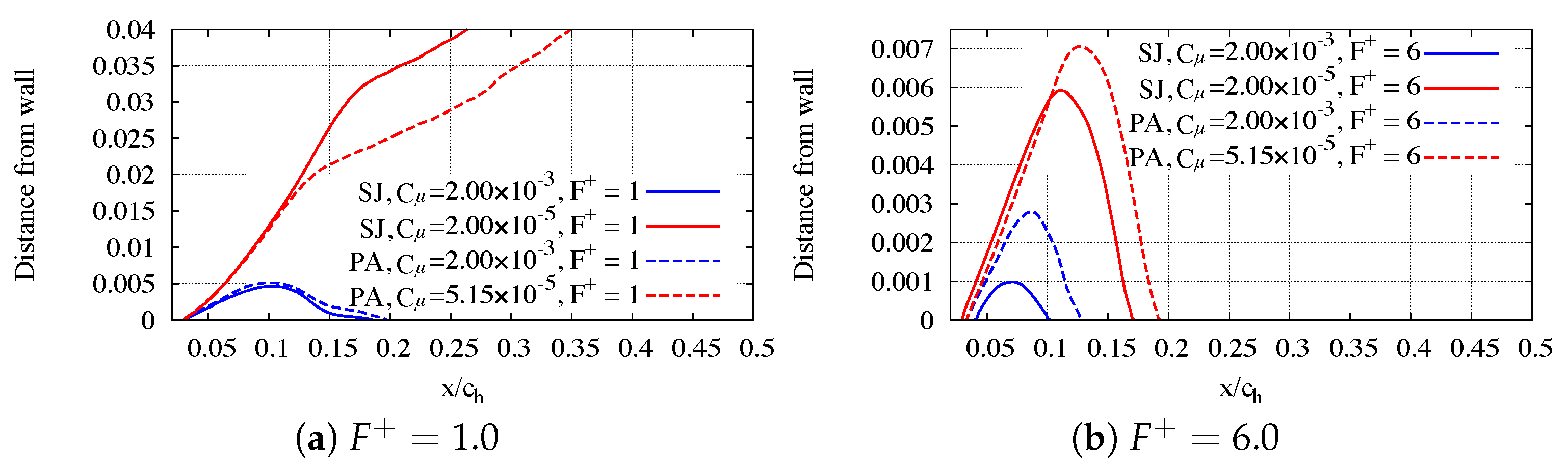
4.2. Capabilities of Separation Control

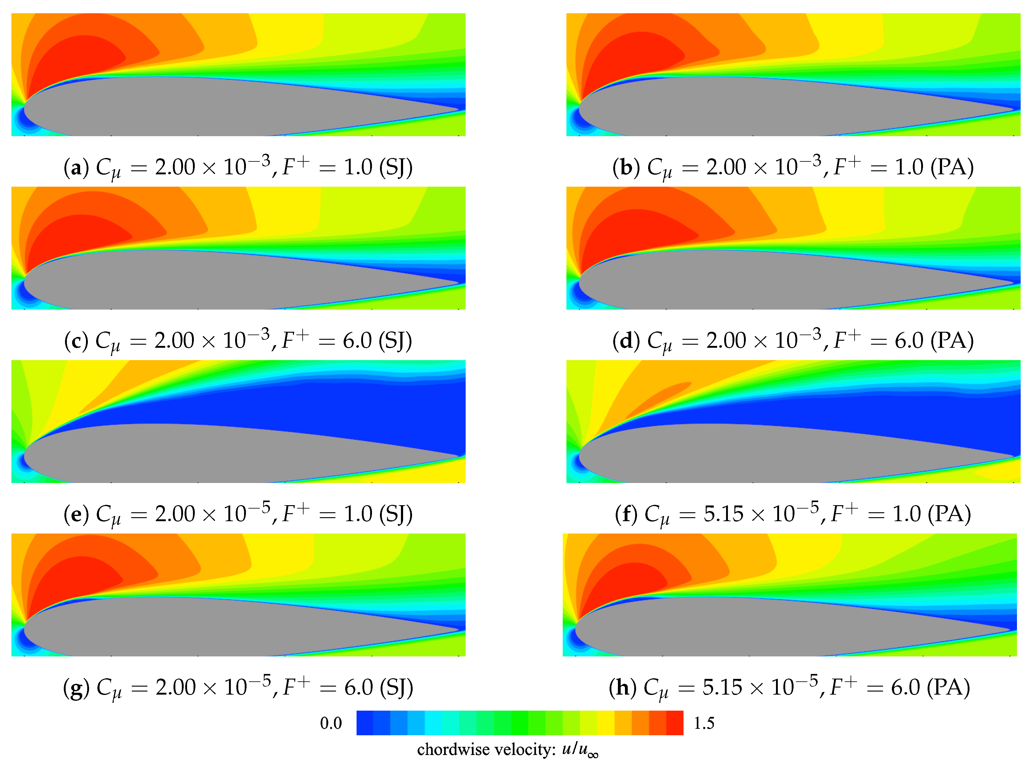
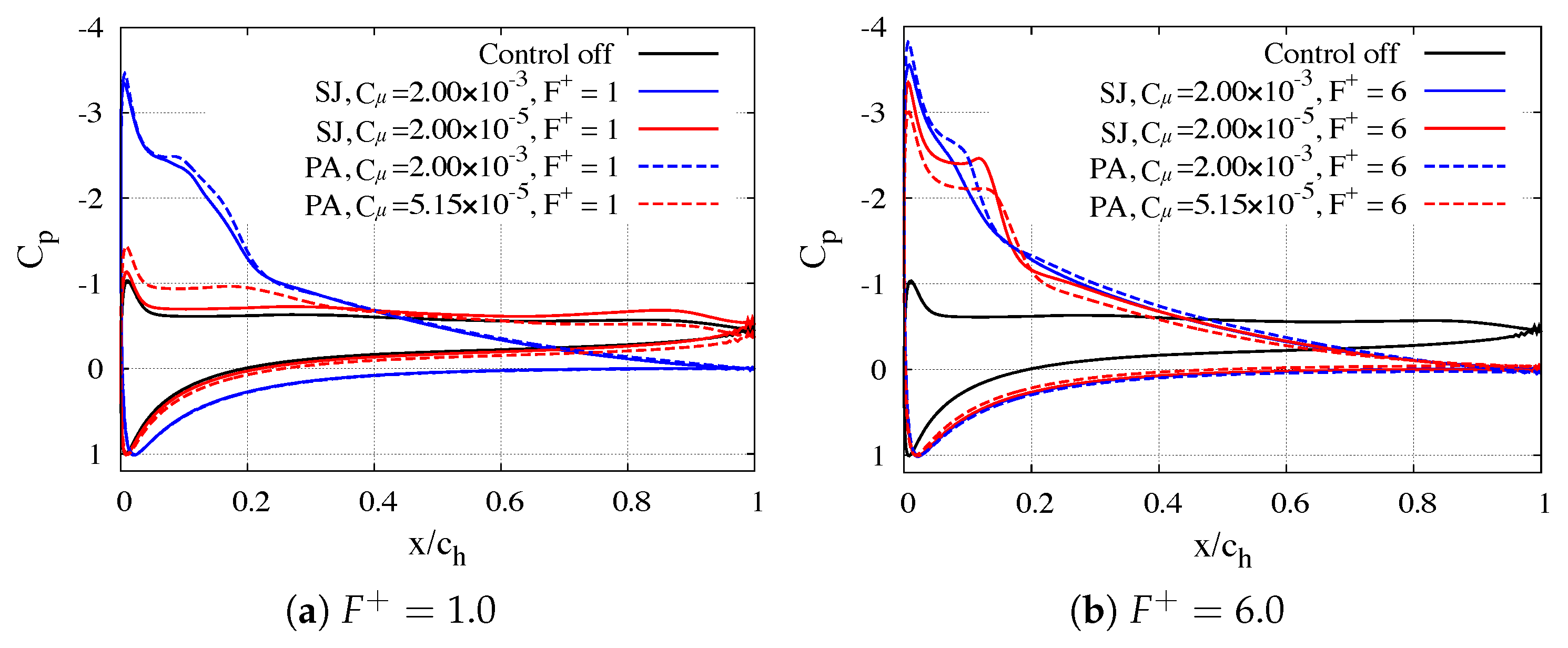
4.3. Flow Fields of Controlled Cases


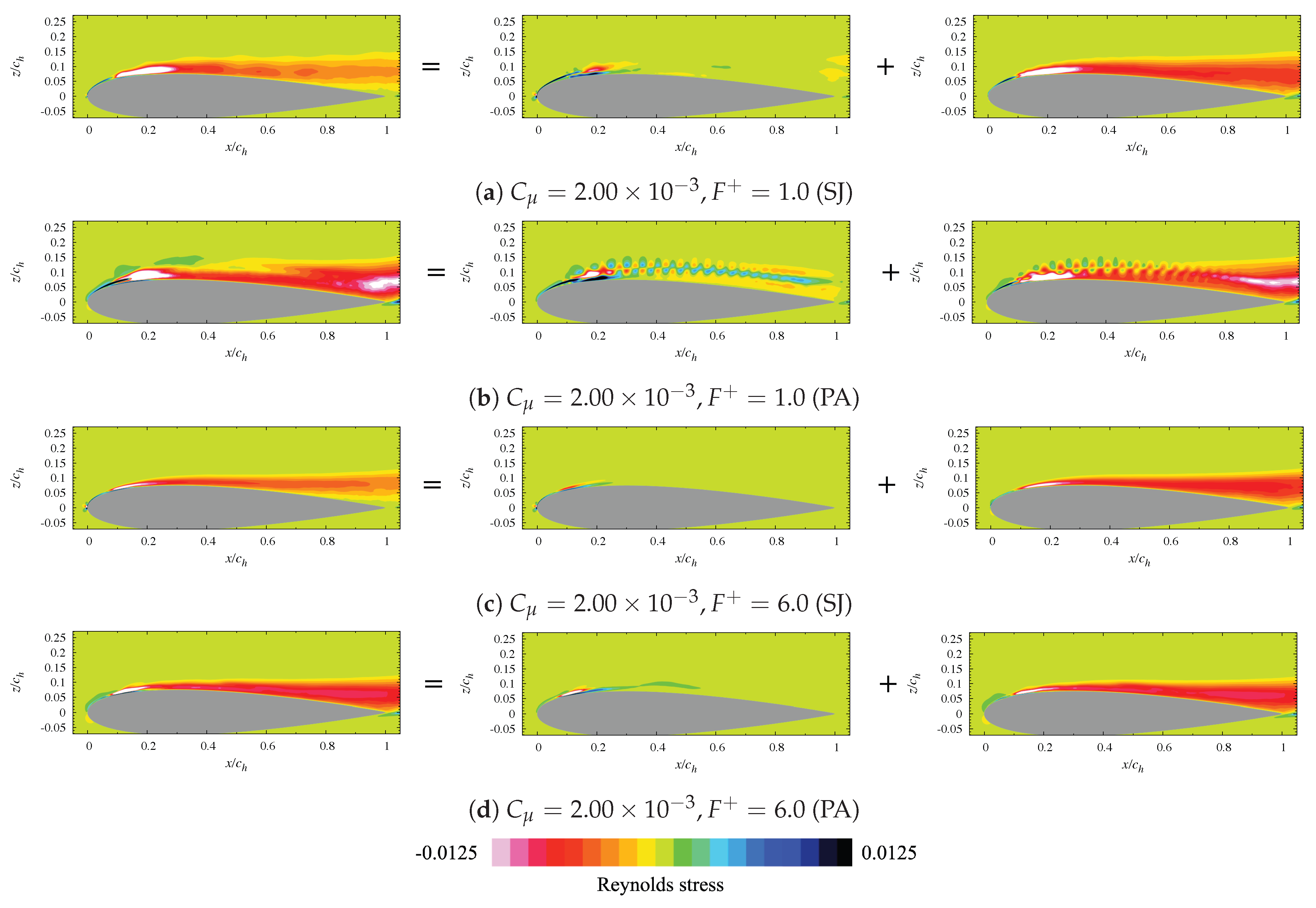
4.4. Phase Decomposition of Turbulent Statistics


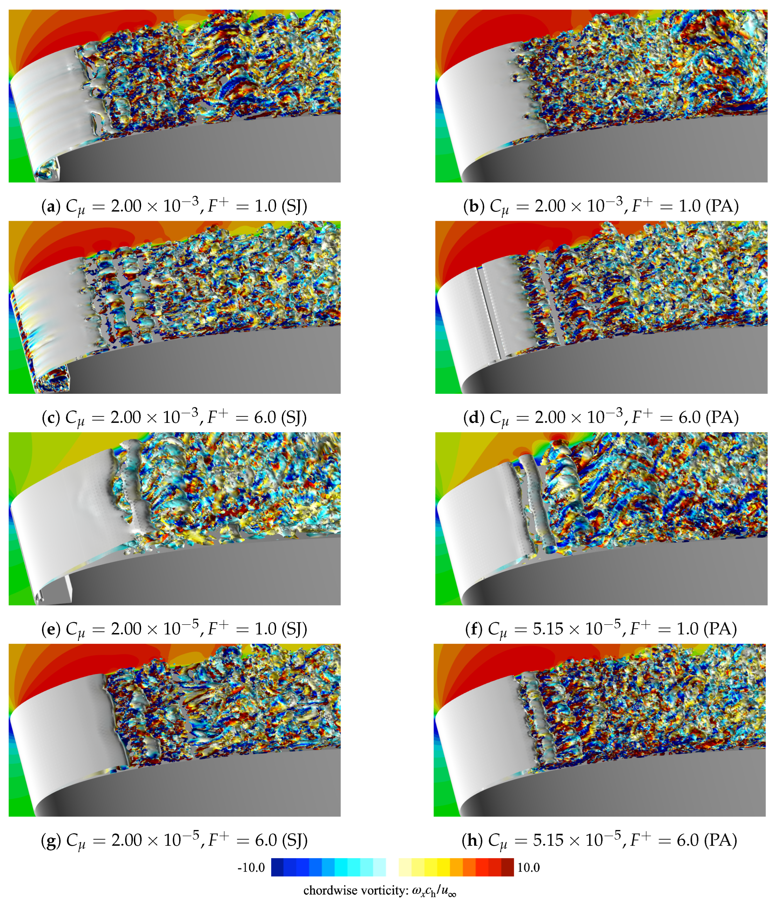
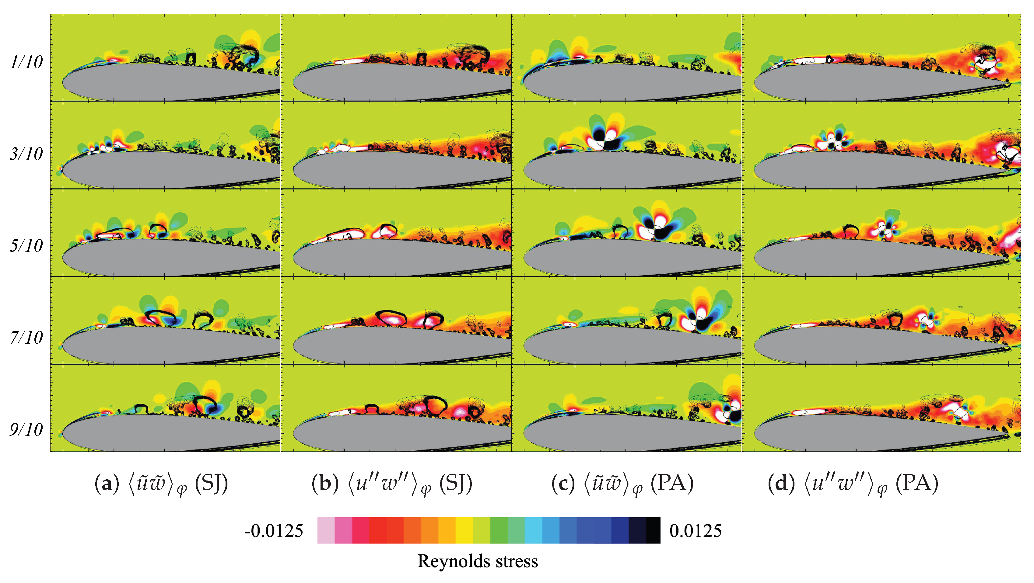
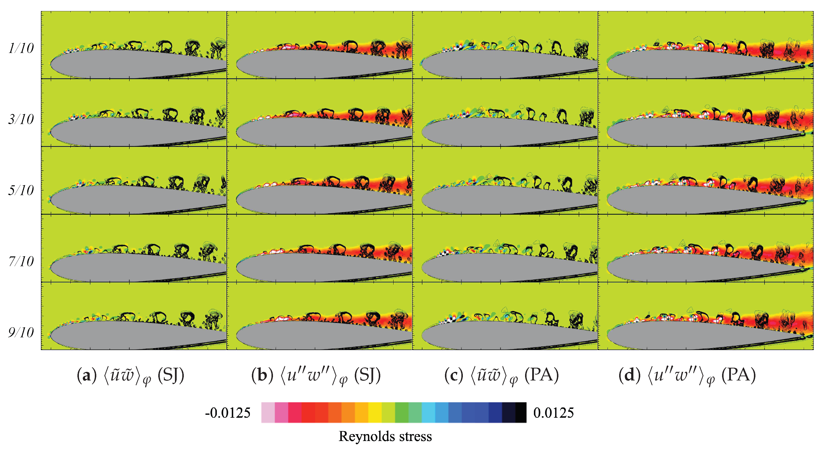
4.5. Coherent Vortex Structures and Chordwise Momentum Exchange in Phase-Averaged Flow Fields


5. Conclusions
- A.
- Wall-tangential velocity;
- B.
- Three-dimensional flow structures;
- C.
- Spatial locality;
- D.
- Temporal fluctuation.
Author Contributions
Funding
Institutional Review Board Statement
Informed Consent Statement
Data Availability Statement
Conflicts of Interest
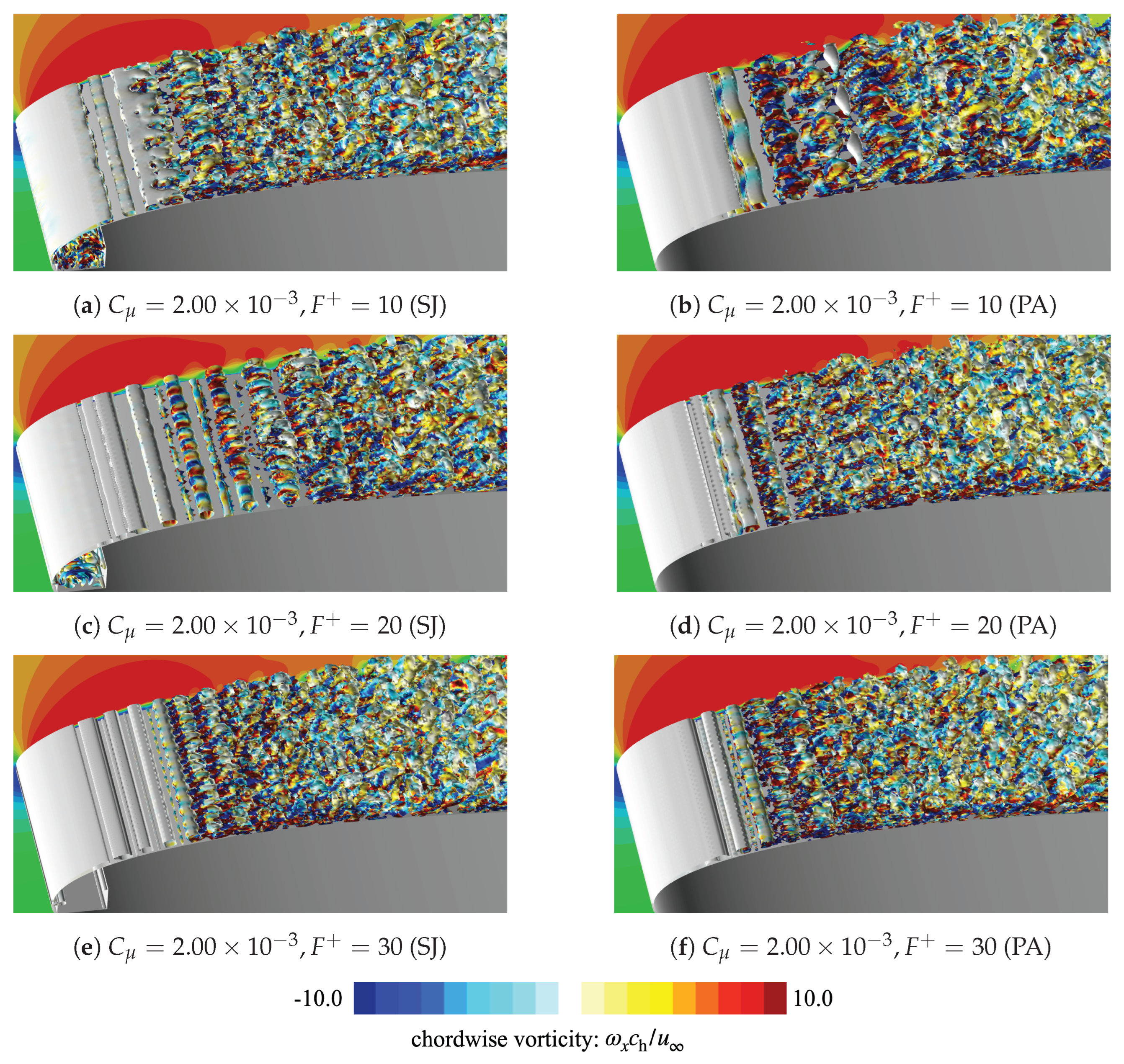
Appendix A. Results of Higher F+ Actuation


References
- Greenblatt, D.; Wygnanski, I.J. The control of flow separation by periodic excitation. Prog. Aerosp. Sci. 2000, 36, 487–545. [Google Scholar] [CrossRef]
- Cattafesta, L.N., III; Sheplak, M. Actuators for active flow control. Annu. Rev. Fluid Mech. 2011, 43, 247–272. [Google Scholar] [CrossRef] [Green Version]
- Greenblatt, D.; Williams, D.R. Flow Control for Unmanned Air Vehicles. Annu. Rev. Fluid Mech. 2022, 54, 383–412. [Google Scholar] [CrossRef]
- Smith, B.L.; Glezer, A. The formation and evolution of synthetic jets. Phys. Fluids 1998, 10, 2281. [Google Scholar] [CrossRef]
- Chen, F.; Yao, C.; Beeler, G.; Bryant, R.; Fox, R. Development of synthetic jet actuators for active flow control at NASA Langley. In Proceedings of the Fluids 2000 Conference and Exhibit, Denver, CO, USA, 19–22 June 2000. [Google Scholar]
- Smith, B.L.; Glezer, A. Jet vectoring using synthetic jets. J. Fluid Mech. 2002, 458, 1–34. [Google Scholar] [CrossRef]
- Amitay, M.; Glezer, A. Role of Actuation Frequency in Controlled Flow Reattachment over a Stalled Airfoil. AIAA J. 2002, 40, 209–216. [Google Scholar] [CrossRef]
- Okada, K.; Oyama, A.; Fujii, K.; Miyaji, K. Computational Study of Effects of Nondimensional Parameters on Synthetic Jets. Trans. Jpn. Soc. Aeronaut. Space Sci. 2012, 55, 1–11. [Google Scholar] [CrossRef] [Green Version]
- Zhang, W.; Samtaney, R. A direct numerical simulation investigation of the synthetic jet frequency effects on separation control of low-Re flow past an airfoil. Phys. Fluids 2015, 27, 055101. [Google Scholar] [CrossRef] [Green Version]
- Abe, Y.; Nonomura, T.; Fujii, K. Flow instability and momentum exchange in separation control by a synthetic jet. Phys. Fluids 2023, 35, 065114. [Google Scholar]
- Corke, T.; Post, M.; Orlov, D. Single dielectric barrier discharge plasma enhanced aerodynamics: Physics, modeling and applications. Exp. Fluids 2009, 46, 1–26. [Google Scholar] [CrossRef]
- Corke, T.C.; Enloe, C.L.; Wilkinson, S.P. Dielectric Barrier Discharge Plasma Actuators for Flow Control. Annu. Rev. Fluid Mech. 2010, 42, 505–529. [Google Scholar] [CrossRef]
- Sato, M.; Nonomura, T.; Okada, K.; Asada, K.; Aono, H.; Yakeno, A.; Abe, Y.; Fujii, K. Mechanisms for Laminar Separated-Flow Control using DBD Plasma Actuator at Low Reynolds Number. Phys. Fluids 2015, 27, 117101. [Google Scholar] [CrossRef]
- Pescini, E.; Marra, F.; De Giorgi, M.G.; Francioso, L.; Ficarella, A. Investigation of the boundary layer characteristics for assessing the DBD plasma actuator control of the separated flow at low Reynolds numbers. Exp. Therm. Fluid Sci. 2017, 81, 482–498. [Google Scholar] [CrossRef]
- Sato, M.; Okada, K.; Asada, K.; Aono, H.; Nonomura, T.; Fujii, K. Unified mechanisms for separation control around airfoil using plasma actuator with burst actuation over Reynolds number range of 103–106. Phys. Fluids 2020, 32, 025102. [Google Scholar] [CrossRef]
- Yarusevych, S.; Kotsonis, M. Effect of Local DBD Plasma Actuation on Transition in a Laminar Separation Bubble. Flow Turbul. Combust. 2017, 98, 195–216. [Google Scholar] [CrossRef]
- Ziadé, P.; Feerob, M.A.; Sullivanc, P.E. A numerical study on the influence of cavity shape on synthetic jet performance. Int. J. Heat Fluid Flow 2018, 74, 187–197. [Google Scholar] [CrossRef]
- Kral, L.D.; Donovan, J.F.; Cain, A.B.; Cary, A.W. Numerical simulation of synthetic jet actuators. In Proceedings of the 4th Shear Flow Control Conference, Snowmass Village, CO, USA, 29 June–2 July 1997. [Google Scholar]
- Smith, B.L.; Glezer, A. Vectoring and small-scale motions effected in free shear flows using synthetic jet actuators. In Proceedings of the 35th Aerospace Sciences Meeting and Exhibit, Reno, NV, USA, 6–9 January 1997. [Google Scholar]
- Yoshioka, S.; Obi, S.; Masuda, S. Turbulence Statistics of peridically perturbed separated flow over backward-facing step. Int. J. Heat Fluid Flow 2001, 22, 393–401. [Google Scholar] [CrossRef]
- Feero, M.A.; Goodfellow, S.D.; Lavoie, P.; Sullivan, P.E. Flow Reattachment Using Synthetic Jet Actuation on a Low-Reynolds-Number Airfoil. AIAA J. 2015, 53, 2005–2014. [Google Scholar] [CrossRef]
- Visbal, M.R. Numerical Exploration of Flow Control for Delay of Dynamic Stall on a Pitching Airfoil. In Proceedings of the 32nd AIAA Applied Aerodynamics Conference, Atlanta, GA, USA, 16–20 June 2014. [Google Scholar]
- Lilley, A.J.; Roy, S.; Visbal, M.R. On the effect of high-frequency plasma actuator forcing for prevention of dynamic stall. In Proceedings of the AIAA SCITECH 2023 Forum, National Harbor, MD, USA, 23–27 January 2023. [Google Scholar]
- Asada, K.; Ninomiya, Y.; Oyama, A.; Fujii, K. Airfoil Flow Experiment on the Duty Cycle of DBD Plasma Actuator. In Proceedings of the 47th AIAA Aerospace Sciences Meeting including The New Horizons Forum and Aerospace Exposition, Orlando, FL, USA, 5–8 January 2009. [Google Scholar]
- Yarusevych, S.; Kotsonis, M. Steady and transient response of a laminar separation bubble to controlled disturbances. J. Fluid Mech. 2017, 813, 955–990. [Google Scholar] [CrossRef]
- Kurelek, J.W.; Yarusevych, S.; Kotsonis, M. Vortex merging in a laminar separation bubble under natural and forced conditions. Phys. Rev. Fluids 2019, 4, 063903. [Google Scholar] [CrossRef] [Green Version]
- Marxen, O.; Kotapati, R.B.; Mittal, R.; Zaki, T. Stability analysis of separated flows subject to control by zero-net-mass-flux jet. Phys. Fluids 2015, 27, 68–89. [Google Scholar] [CrossRef] [Green Version]
- Lambert, A.; Yarusevych, S. Effect of angle of attack on vortex dynamics in laminar separation bubbles. Phys. Fluids 2019, 31, 064105. [Google Scholar] [CrossRef]
- Sekimoto, S.; Fujii, K.; Anyoji, M.; Miyakawa, Y.; Ito, S.; Shimomura, S.; Nishida, H.; Nonomura, T.; Matsuno, T. Flow Control around NACA0015 Airfoil Using a Dielectric Barrier Discharge Plasma Actuator over a Wide Range of the Reynolds Number. Actuators 2023, 12, 43. [Google Scholar] [CrossRef]
- You, D.; Moin, P. Active control of flow separation over an airfoil using synthetic jets. J. Fluids Struct. 2008, 24, 1349–1357. [Google Scholar] [CrossRef]
- Benton, S.I.; Visbal, M.R. Extending the Reynolds Number Range of High-Frequency Control of Dynamic Stall. AIAA J. 2019, 57, 2676–2681. [Google Scholar] [CrossRef]
- Aono, H.; Sekimoto, S.; Sato, M.; Yakeno, A.; Nonomura, T.; Fujii, K. Computational and experimental analysis of flow structures induced by a plasma actuator with burst modulations in quiescent air. Mech. Eng. J. 2015, 2, 15-00233. [Google Scholar] [CrossRef] [Green Version]
- Suzen, Y.B.; Huang, P.G.; Jacob, J.D.; Ashpis, D.E. Numerical Simulations of Plasma Based Flow Control Application. In Proceedings of the 35th AIAA Fluid Dynamics Conference and Exhibit, Toronto, ON, Canada, 6–9 June 2005. [Google Scholar]
- Lilley, A.; Roy, S.; Michels, L.; Roy, S. Performance recovery of plasma actuators in wet conditions. J. Phys. Appl. Phys. 2022, 55, 155201. [Google Scholar] [CrossRef]
- Tanaka, M.; Kubo, N.; Kawabata, H. Plasma actuation for leading edge separation control on 300-kW rotor blades with chord length around 1 m at a Reynolds number around 1.6×10⁶. J. Phys. Conf. Ser. 2020, 1618, 052013. [Google Scholar] [CrossRef]
- Wicks, M.; Thomas, F. Effect of Relative Humidity on Dielectric Barrier Discharge Plasma Actuator Body Force. AIAA J. 2015, 53, 2801–2805. [Google Scholar] [CrossRef]
- Avino, F.; Howling, A.A.; Allmen, M.V.; Waskow, A.; Ibba, L.; Han, J.; Furno, I. Surface DBD degradation in humid air, and a hybrid surface-volume DBD for robust plasma operation at high humidity. J. Phys. D Appl. Phys. 2023, 56, 345201. [Google Scholar] [CrossRef]
- Weigel, P.; Schuller, M.; Gratias, A.; Lipowski, M.; ter Meer, T.; Bardet, M. Design of a synthetic jet actuator for flow separation control. CEAS Aeronaut. J. 2020, 11, 813–821. [Google Scholar] [CrossRef]
- Fujii, K.; Endo, H.; Yasuhara, M. Activities of Computational Fluid Dynamics in Japan: Compressible Flow Simulations, High Performance Computing Research and Practice in Japan; John Wiley & Sons: Hoboken, NJ, USA, 1990. [Google Scholar]
- Date, S.; Abe, Y.; Okabe, T. Effects of fiber properties on aerodynamic performance and structural sizing of composite aircraft wings. Aerosp. Sci. Technol. 2023, 124, 107565. [Google Scholar] [CrossRef]
- Lele, S.K. Compact Finite Difference Schemes with Spectral-like Resolution. J. Comput. Phys. 1992, 103, 16–42. [Google Scholar] [CrossRef]
- Abe, Y.; Iizuka, N.; Nonomura, T.; Fujii, K. Conservative metric evaluation for high-order finite difference schemes with the GCL identities on moving and deforming grids. J. Comput. Phys. 2013, 232, 14–21. [Google Scholar] [CrossRef]
- Abe, Y.; Iizuka, N.; Nonomura, T.; Fujii, K. Geometric interpretations and spatial symmetry property of metrics in the conservative form for high-order finite-difference schemes on moving and deforming grids. J. Comput. Phys. 2014, 260, 163–203. [Google Scholar] [CrossRef]
- Gaitonde, D.V.; Visbal, M.R. Padé-Type Higher-Order Boundary Filters for the Navier-Stokes Equations. AIAA J. 2000, 38, 2103–2112. [Google Scholar] [CrossRef]
- Visbal, M.R.; Rizzetta, D.P. Large-eddy Simulation on General Geometries Using Compact Differencing and Filtering Schemes. In Proceedings of the 40th AIAA Aerospace Sciences Meeting & Exhibit, Reno, NV, USA, 14–17 January 2002. [Google Scholar]
- Visbal, M.R.; Morgan, P.E.; Rizzetta, D.P. An Implicit LES Approach Based on High-Order Compact Differencing and Filtering Schemes. In Proceedings of the 16th AIAA Computational Fluid Dynamics Conference, Orlando, FL, USA, 23–26 June 2003. [Google Scholar]
- Fujii, K. Unified Zonal Method Based on the Fortified Solution Algorithm. J. Comput. Phys. 1995, 118, 92–108. [Google Scholar] [CrossRef]
- Melville, R.B.; Moiton, S.A.; Rizzetta, D.P. Implementation of a fully-implicit, aeroelastic Navier-Stokes solver. In Proceedings of the 13th Computational Fluid Dynamics Conference, Snowmass Village, CO, USA, 29 June–2 July 1997. [Google Scholar]
- Fujii, K. High-performance computing-based exploration of flow control with micro devices. Phylosophical Trans. R. Soc. A 2014, 372, 20130326. [Google Scholar] [CrossRef] [Green Version]
- Nishida, H.; Nonomura, T.; Abe, T. Three-dimensional simulations of discharge plasma evolution on a dielectric barrier discharge plasma actuator. J. Appl. Phys. 2014, 115, 133301. [Google Scholar] [CrossRef]
- Benard, N.; Moreau, E. Electrical and mechanical characteristics of surface AC dielectric barrier discharge plasma actuators applied to air flow control. Exp. Fluids 2014, 55, 1846. [Google Scholar] [CrossRef] [Green Version]


| Case Name | Input Momentum () | |
|---|---|---|
| strong input (SJ) | 1.0, 6.0, 10, 15, 20, 30 | |
| strong input (PA) | 1.0, 6.0, 10, 15, 20, 30 | |
| weak input (SJ) | 1.0, 6.0, 10, 15, 20, 30 | |
| weak input (PA) | 1.0, 6.0, 10, 15, 20, 30 |
| Zone Name | Description | Number of Grid Points | |||
|---|---|---|---|---|---|
| Zone 1 | airfoil grid | 795 | 134 | 179 | 19,068,870 |
| Zone 2 | intermediate grid | 253 | 134 | 91 | 3,085,082 |
| Zone 3 | orifice grid | 45 | 134 | 75 | 452,250 |
| Zone 4 | cavity grid | 157 | 134 | 214 | 4,502,132 |
Disclaimer/Publisher’s Note: The statements, opinions and data contained in all publications are solely those of the individual author(s) and contributor(s) and not of MDPI and/or the editor(s). MDPI and/or the editor(s) disclaim responsibility for any injury to people or property resulting from any ideas, methods, instructions or products referred to in the content. |
© 2023 by the authors. Licensee MDPI, Basel, Switzerland. This article is an open access article distributed under the terms and conditions of the Creative Commons Attribution (CC BY) license (https://creativecommons.org/licenses/by/4.0/).
Share and Cite
Abe, Y.; Nonomura, T.; Sato, M.; Aono, H.; Fujii, K. Comparison of Separation Control Mechanisms for Synthetic Jet and Plasma Actuators. Actuators 2023, 12, 322. https://doi.org/10.3390/act12080322
Abe Y, Nonomura T, Sato M, Aono H, Fujii K. Comparison of Separation Control Mechanisms for Synthetic Jet and Plasma Actuators. Actuators. 2023; 12(8):322. https://doi.org/10.3390/act12080322
Chicago/Turabian StyleAbe, Yoshiaki, Taku Nonomura, Makoto Sato, Hikaru Aono, and Kozo Fujii. 2023. "Comparison of Separation Control Mechanisms for Synthetic Jet and Plasma Actuators" Actuators 12, no. 8: 322. https://doi.org/10.3390/act12080322