Development of an Adaptive Fuzzy Sliding Mode Controller of an Electrohydraulic Actuator Based on a Virtual Prototyping

Abstract

The EHA (electro hydraulic actuator) has a notable advantage over conventional hydraulic actuators as it uses a closed-loop circuit, reducing the size and volume of oil, and eliminates pressure losses caused by valve orifices. However, accurate control performance of EHA is difficult to achieve using a traditional PID (proportional integral derivative) controller due to the strongly nonlinear, time-varying, and unknown dynamics of the system. Hence this paper seeks to address this problem by proposing a design of an intelligent controller for the EHA. The proposed adaptive fuzzy sliding mode controller (AFSMC) is developed as a hybrid of the adaptive, fuzzy logic, and sliding mode algorithms. To reduce costs and time, a virtual prototype approach is also proposed instead of experimentations to evaluate the performance of the proposed controller. The virtual model of the EHA is built in Amesime software, and then embedded into Matlab/Simulink where the AFSMC is developed and tested to obtain the position responses of the EHA. The results show that the AFSMC is highly successful and more efficient than the traditional PID at controlling the position of the piston accurately.

1. Introduction

Hydrostatic transmission systems are commonly used in the industry such as in vehicles and machineries that utilize hydraulic fluid to transmit power. They are able to provide high power, low inertia, reliability, and flexibility in terms of changing the transmission ratio, and are easy to automate. Hydraulic systems are typically classified into either open-loop or closed-loop circuits. Studies on valve-controlled open-loop systems have shown problems of pressure drops and leakages at control valves, resulting in energy wastage [1,2,3]. On the other hand, closed-loop circuits offer increased transmission efficiency by eliminating the need for directional control valves. Past investigations have utilized direct control of the hydraulic actuator by the operation of the pump [4,5]. Thus, a closed-loop circuit is more efficient in transmitting power to generate high force or torque in the actuator than an open-loop circuit. Using electro-hydraulic actuators (EHAs), power can be transferred from the high speed of an electric motor to the high force of a hydraulic cylinder [6]. A closed-loop hydraulic circuit has demonstrated high working efficiency of 60% to 68.2% in an energy regeneration system of the boom for a hydraulic excavator [7]. The development of the EHA has progressed from applications in research projects [8,9] up to the commercialization stage [10].

The precise dynamic modeling of the EHA is particularly challenging as it is a highly nonlinear and uncertain system. Furthermore, it is arduous to estimate the system parameters accurately, particularly in practical situations, heightening the challenge of implementing model-based control algorithms for governing the position of the actuator. While a sliding mode control algorithm is a useful approach for nonlinear systems [11], the conventional sliding mode control method requires a precise dynamic model of the system [12]. Thus, researchers have proposed several control strategies to solve these difficulties. Cheng and Shanan designed an adaptive time-varying sliding control for a hydraulic servo system [13]. A self-tuning control strategy to manage a low-friction pneumatic actuator under the influence of gravity was presented by Richardson, Plummer, and Brown [14]. Guan and Pan proposed and successfully tested an adaptive sliding mode controller for the electro-hydraulic system [15], while Acarman, Hatipoglu, and Ozguner suggested a feedback-linearization control strategy with consideration for various states of the chamber pressure in the system model [16]. Additionally, a fuzzy control technique can act as a useful tool for nonlinear structures without model-based requirements [17,18]. However, traditional fuzzy controllers depend on the expert or operator’s experience, making it difficult to design an effective fuzzy logic controller.

To overcome the limitations of conventional PID algorithms when managing systems with dynamic uncertainty, several researchers have proposed hybrid controllers that combine the fuzzy logic control algorithm with PID, sliding mode, or neural network controls [19,20]. For example, Zhao, Chen, Dian, Guo, and Li [21] proposed applying type-2 fuzzy logic to estimate PID controller parameters online for controlling power-line inspection (PLI) robot systems. In another study, Phu, Hung, Ahmadian, and Senu [22] designed an intelligent controller based on the combination of the fuzzy-PID controller and a fuzzy control differential equation. Ursu, Tecuceanu, Toader, Calinoiu, Ursu, and Berar [23] proposed a novel solution for the positioning of the outer loop of a hydrostatic type servo actuator using an application of the neuro-fuzzy control rule. During their research, they investigated the fundamental issues related to the control of hydrostatic EHA systems. The team conducted experiments by supplying hydraulic oil from a fixed displacement, bidirectional Haldex hydraulic gear pump to the cylinder doublet, which consists of two single-acting parts. The results of their study underscore the remarkable effectiveness of the neuro-fuzzy control algorithm, which ensured optimal dynamic behavior of the hydrostatic servo actuator, paving the way for innovative solutions in the field.

To significantly improve the energy efficiency of hydraulic systems, innovative hydraulic architectures must be developed that allow components to operate in high efficiency regions. Vukovic and Murrenhoff [24] developed a comprehensive classification barcode with a comprehensive range of standard analog and state-of-the-art digital hydraulic components. This barcode has been implemented in two major research projects, one on mobile hydraulic systems for excavators and the other on switched displacement hydrostatic transmissions for wind turbines, successfully achieving significant improvements in energy efficiency. Yordanov, Ormandzhiev, and Mihalev [25] also made commendable progress in the field of hydraulic system control by implementing benchmarking results of control quality using standard fuzzy controllers and classical PI controllers in an experimental electrohydraulic servo system. These controllers were compared based on various quality indicators with two input thermals (error and error derivative) and three input thermals (error, first error derivative, and output derivative). Such important advances in hydraulic system architecture and control will revolutionize the field with newfound efficiency and precision. Chen, Liu, Jia, Qiu, and Yu, et al. [26] introduced a breakthrough nonlinear adaptive backstepping control technique to address the highly relevant system parameter uncertainty problem that arises in the position control process of an electrohydraulic servo closed-loop pump control system. Their approach deals with the parameter uncertainty of the nonlinear system by setting the adaptive rate of the uncertain parameter. This modifies the parameter disturbance online in real time, thus improving the accuracy and robustness of the control system. Experimental tests on a pump control system platform have verified the feasibility of the controller, with impressive results confirming the effectiveness of the proposed control strategy. The pump control system can now be effortlessly controlled with high precision, demonstrating a steady-state control accuracy of ±0.02 mm, providing an encouraging basis for the technical application and promotion of the pump control system. Similarly, Rybarczyk and Milecki [27] proposed some modifications to improve both the dynamics of an electrohydraulic servo drive and the adaptation to load forces, thus reducing energy consumption. They described the application of the model following control (MFC) method to the control of an electrohydraulic servo drive with a unique proportional valve designed with a permanent magnet synchronous motor (PMSM). To validate the effectiveness of their method, they proposed a theoretical description of the drive, modeled and tested using simulations. Laboratory investigations were also conducted to compare the simulation results with real-world tests. It was shown that the use of MFC significantly reduces the settling time of the drive and improves its overall dynamics. Overall, these significant advances are game changers in the field of electrohydraulic systems, and their implications will undoubtedly continue to drive progress and achievements in the field.

Ren, Mou, Wen, and Chen [28] made remarkable progress by synthesizing a position controller using quantitative feedback theory (QFT) for a single-rod EHA while considering the tolerance to internal actuator leakage, different loads, and environmental stiffness. Comparing their fault-tolerant controller with another QFT controller synthesized without considering the leakage fault, the simulation results showed that the fault-tolerant QFT controller could achieve the prescribed specifications even with internal leakage up to 8.6 L/min, thus confirming its effectiveness and reliability. Similarly, Sun, Dong, Wang, and Li [29] proposed dynamic models for the valve-controlled asymmetric hydraulic cylinder, and a simplified mathematical model of the electrohydraulic position servo system was determined by ignoring the nonlinear factors of the servo valve. They designed a novel sliding mode control (SMC) method based on the adaptive reaching law to control the displacement and velocity of the piston. Through comparative analysis of the SMC controller with the traditional exponential reaching law and the adaptive reaching law, their Amesim/Simulink co-simulation results confirmed that this method significantly suppressed the sliding mode chatter of the electrohydraulic position servo system. These cutting-edge advances lead to significant improvements in the integrity, efficiency, and reliability of hydraulic systems.

This study proposes the development of an adaptive fuzzy sliding mode controller for regulating the position tracking of the electro-hydraulic actuator (EHA), leveraging on virtual prototyping technology to visualize the system performance. The proposed controller employs a finite combination of basic functions to represent two unknown time-varying functions into which the system uncertainties have been lumped together. Furthermore, a fuzzy logic inference mechanism removes the chattering issue from conventional sliding mode control by employing a hitting control law. Currently, thanks to the robust development of engineering software, virtual prototyping technology can simulate and evaluate real system performance without experiments, lowering manufacturing costs and errors while ensuring product quality [30,31,32,33,34,35,36]. The tracking control performance of the EHA is evaluated through a virtual model created using Amesim software.

This paper is structured as follows: In Section 2, we present the modeling of the EHA. Then, based on the dynamic model, Section 3 outlines the design of an adaptive fuzzy sliding mode controller. Section 4 presents the virtual model and simulation results, and finally, Section 5 concludes with the findings of the study.

2. Modeling of Electro-Hydraulic Actuator

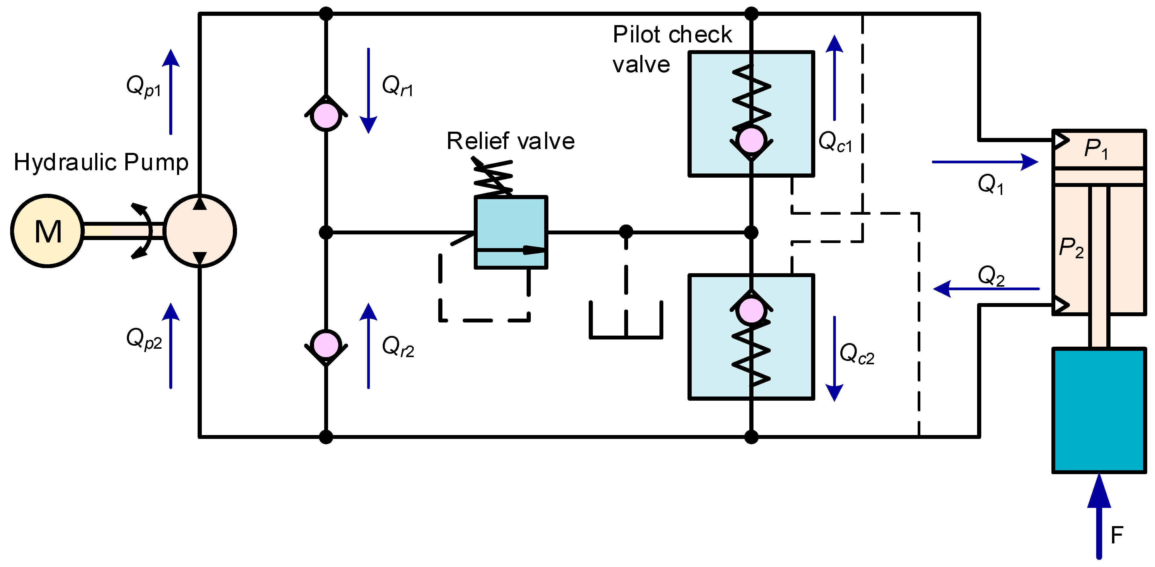
The operational mechanics of the electro-hydraulic actuator involves a closed-loop hydraulic circuit that eliminates pressure loss caused by valve orifice areas (Figure 1). However, due to the hydraulic cylinder’s asymmetry, two pilot-operated check valves are required to provide supplementary oil volume from the tank or discharge oil volume to the tank. In addition, a relief valve controls the system’s pressure through two check valves devoid of springs. The AC servo adjusts the flow rate of the bidirectional pump and fluid flow direction, with regulation performed via an adaptive fuzzy sliding mode controller.

The piston’s dynamics can be described using Newton’s second law of motion, as follows:

$$m\cdot \ddot{x}+c\dot{x}=A_p{P}_1-F-\left(A_p-a\right)P_2$$

(1)

where, m (mass, kg), c (damping coefficient, N.s/m), A_p (effective area of the piston), a (area of the rod, in m²), P₁ and P₂ (pressure in the two chambers, Pa, depicted in Figure 1), and F (the externally applied load exerting on the cylinder, N).

Utilizing the fundamental principles of hydraulic transmission, the pressure in the working chamber can be calculated as shown in Equation (2).

$$\begin{array}{l}{\dot{P}}_1=\frac{\beta }{A_{p}x+V_{01}}\left(Q_1-\frac{1}{R_i}\left(P_1-P_2\right)-A_p\dot{x}\right)\\ {\dot{P}}_2=\frac{\beta }{-\left(A_p-a\right)x+V_{02}}\left(\frac{1}{R_i}\left(P_1-P_2\right)-Q_2+\left(A_p-a\right)\dot{x}\right)\end{array}$$

(2)

where, the original volumes of the two chambers are represented by V₀₁ and V₀₂, and R_i denotes the cylinder’s internal leakage resistance (i = 1, 2), which depends on the contact length between the piston and the cylinder, the diameter of the piston, the oil viscosity, and the radius clearance. Increasing the value of R_i lowers the leakage between two chambers of the cylinder. The flow rate (Q₁) entering chamber 1 and the flow rate (Q₂) leaving the remaining chamber are calculated using Equation (3).

$$\begin{array}{l}{Q}_1=-Q_{r1}+Q_{p1}+Q_{c1}\\ Q_2=\frac{A_p-a}{A_p}{Q}_1=-Q_{c2}+Q_{p2}+Q_{r2}\end{array}$$

(3)

The flow rate passing through the pilot-operated check valves 1 and 2 are denoted as Q_c1 and Q_c2, respectively. Conversely, the check valves without a spring that return to the tank are associated with Q_r1 and Q_r2 flow rates. Q_p1 and Q_p2 are the flow rates at the outlet and inlet of the pump, measured in m³/s. The flow rate supplied by the bidirectional pump is calculated by utilizing Equation (4).

$$Q_{p1}=-Q_{p2}={\eta }_v\cdot D\cdot \omega$$

(4)

where D is the oil volume leaving the outlet of the pump, measured in m³/rev, while the speed of the pump shaft is symbolized by n, measured in rev/s. Additionally, η_v denotes the volumetric efficiency of the pump.

Given y₁ = x, y₂ = $\dot{x}$, and y₃ = $\ddot{x}$, the state space representation of Equations (1)–(4) is of the following form of Equation (5).

$$\left\{\begin{array}{c}{\dot{y}}_1=y_2\\ {\dot{y}}_2=y_3\\ {\dot{y}}_3=-\frac{1}{m}\left[\left(A_p-a\right){\dot{P}}_2+\dot{F}+c{y}_2-A_p{\dot{P}}_1\right]\end{array}\right.$$

(5)

Close inspection of Equations (2)–(5) shows that the system’s state can be modified by managing the speed of the bidirectional pump powered by the AC servo motor. Thus, this reflects the primary aim of this study in developing a control technique that regulates the speed of the pump’s shaft, thereby achieving precise tracking of the cylinder’s real-time position with respect to its desired position.

3. Controller Design

The traditional sliding mode controller (SMC) is designed based on a dynamic model and has proven to be very effective for nonlinear systems. However, as presented in the previous section, the EHA has unknown and nonlinear dynamic responses. Furthermore, the dynamic model given in Equation (5) is established through simplification by ignoring factors such as friction and oil leakages. Therefore, this traditional algorithm is not easily applicable for EHA. To overcome this issue, the parameters as well as the distribution of the model are lumped as an unknown nonlinear function which is expressed approximately through Fourier series. A modified sliding mode controller is developed in which the adaptive algorithm is used to estimate the equivalent control rule created by the sliding mode controller.

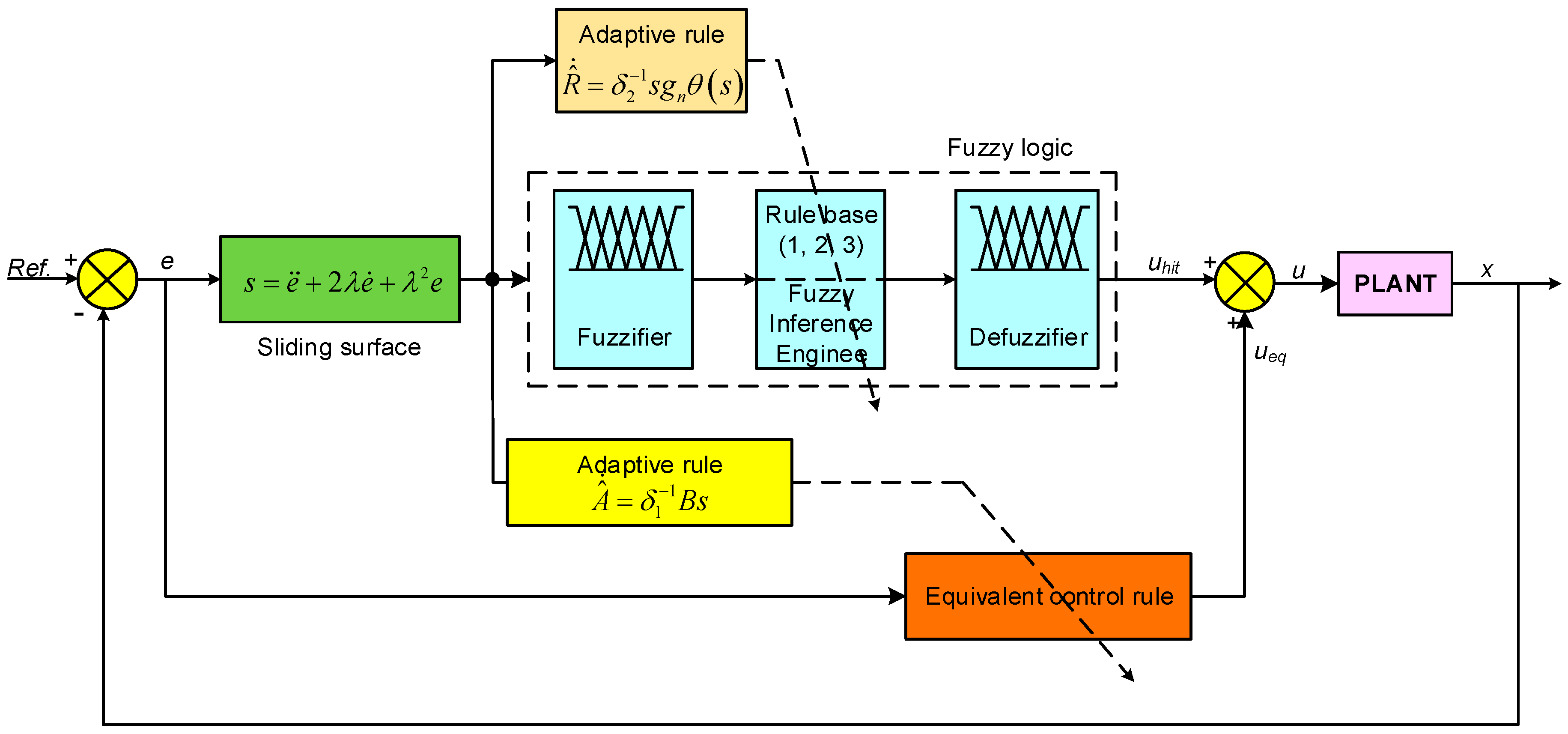
Another disadvantage of the SMC is that the hitting control action is not a continuous function with respect to time. This can cause instability and impairs the control performance. Thus, a fuzzy logic algorithm is proposed to replace the traditional hitting control action. Figure 2 illustrates the comprehensive structure of the controller.

By inserting Equations (3)–(4) into Equation (5), a state-space model is described in the revised Equation (6).

$$\left\{\begin{array}{c}{\dot{y}}_1=y_2\\ {\dot{y}}_2=y_3\\ {\dot{y}}_3=f\left(y_1,y_2,t\right)+g\left(y_1,t\right)u+d\left(t\right)\end{array}\right.$$

(6)

in which,

$$\begin{array}{ll}f\left(y_1,y_2,t\right)=& -\frac{\beta \left(A_p-a\right)}{m\left(V_{02}-\left(A_p-a\right)y_1\right)}\left(\left(A_p-a\right)y_2+\frac{1}{R_i}\left(P_1-P_2\right)\right)-\frac{\beta A_p}{m\left(V_{01}+A_p{y}_1\right)}\left(A_p{y}_2+\frac{1}{R_i}\left(P_1-P_2\right)\right)\\ & -\frac{c}{m}{y}_2\end{array}$$

$$g\left(y_1,t\right)=\left(\frac{\beta {\eta }_{v}D\left(A_p-a\right)}{V_{02}-\left(A_p-a\right)y_1}+\frac{\beta {\eta }_{v}D{A}_p}{V_{01}+A_p{y}_1}\right)$$

$d\left(t\right)=-\dot{F}/m$ is the external distribution

u = ω is the control signal.

Since the absolute pressure inside the working chambers is always larger than the atmosphere pressure, and to ensure the safety of the hydraulic system, the maximum system pressure (P_s) is set by the relief valve. Therefore, the pressure P₁ and P₂ are always smaller than the pressure P_s.

As shown in Equation (6), the function of f(y₁, y₂, t) reveals a dependence on the position, velocity, and pressure, meaning that it is a time varying and continuous function. Additionally, the resistance (R₁ and R₂) to the leakage of the cylinder is difficult to estimate in practical applications. Hence, this function is considered as lumped uncertainty and unknown. Although the parameters of β, η_v, V₀₁, and V₀₂ are not accurately known, their variation range in practical applications can be estimated easily. Thus, the boundary of the function g(y₁, t) can also be easily estimated.

To design the controller, the following assumptions are made:

Assumption 1.

The first assumption states that the function f(y₁, y₂, t) is a continuous unknown time-varying function whose variation boundary is not known. Hence, the function f(y₁, y₂, t) can be estimated utilizing a finite linear combination of fundamental functions, as shown in Equation (7).

$$f\left(y_1,y_2,t\right)=A^T\cdot B+\epsilon$$

(7)

where the simulation time interval is denoted by T, and the parameter and basic function vector are referred to as A and B, respectively. An approximate error of Ɛ is also accounted for in the analysis.

$$A={\left[\begin{array}{cccccc}{a}_0& a_1& b_1& \cdots & a_n& b_n\end{array}\right]}^T$$

$$B={\left[1\hspace{1em}\cos \left(\frac{2\pi }{T}t\right)\hspace{1em}\sin \left(\frac{2\pi }{T}t\right)\hspace{1em}\cdots \hspace{1em}\cos \left(\frac{n2\pi }{T}t\right)\hspace{1em}\sin \left(\frac{n2\pi }{T}t\right)\right]}^T$$

Based on the universal approximation theorem given by [38], there exists a unique parameter vector A^* to minimize the function approximation error. From Equation (7), we have Equation (8) shown as below.

$$f^{*}\left(y_1,y_2,t\right)=A^{*T}\cdot B+\epsilon$$

(8)

Assumption 2.

The function g(y₁, t) is not known, but its boundary is known and can be estimated using Equation (9).

$$0<g_{\min }\le g\left(y_1,t\right)\le g_{\max }$$

(9)

The support for $g\left(t\right)=g_n\Delta g$ based on the fact that g_n is a nominal value that is known, and represents the uncertain value, which is bounded as shown in Equation (10).

$$0<{\beta }_{\min }=\frac{g_{\min }}{g_n}\le \Delta g\le \frac{g_{\max }}{g_n}={\beta }_{\max }$$

(10)

Assumption 3.

The atmospheric pressure and supplied pressure are represented by P_atm and P_s, respectively, and p₁ and p₂ are bounded within the range P_atm ≤ p₁, p₂ ≤ P_s. The AFSMC is derived by defining the sliding surface (s) as follows:

$$s={\left(\frac{d}{dt}+\lambda \right)}^{2}e=\ddot{e}+2\lambda \dot{e}+{\lambda }^{2}e$$

(11)

in which λ is the convergent rate of the error on the sliding surface, where λ > 0. The error (e), which is defined as the difference between the reference value x_ref and the actual response value x of the mass, is used in this context.

$$e=x_{ref}-x$$

(12)

Taking the time derivative of s, which is obtained by inserting Equation (12) into Equation (11), yields the following dynamics for s:

$$\dot{s}={\stackrel{⃛}{x}}_{ref}-{\dot{y}}_3+2\lambda \ddot{e}+{\lambda }^2\dot{e}$$

(13)

To rewrite the dynamics of the signal s, Equations (6) and (8) are substituted into Equation (13):

$$\dot{s}\left(t\right)={\stackrel{⃛}{x}}_{ref}-A^{*T}B-g_{n}u-L\left(t\right)+2\lambda \ddot{e}+{\lambda }^2\dot{e}$$

(14)

where,

$$L\left(t\right)=g_n\left(\Delta g-1\right)u+d\left(t\right)+\epsilon \mathrm{is}\mathrm{called}\mathrm{a}\mathrm{lumped}\mathrm{uncertainty}$$

The equivalent action (u_eq) control strategy can be used to determine the control action required to obtain a solution of $\dot{s}$ = 0, irrespective of the lumped function L(t).

$$u_{eq}=\frac{1}{g_n}\left[{\stackrel{⃛}{x}}_{ref}-A^{*T}B+2\lambda \ddot{e}+{\lambda }^2\dot{e}\right]$$

(15)

The accuracy value of A^* is difficult to obtain in practical application. By introducing $\widehat{A}$ as the estimated parameter vector of A^*, the estimated equivalent action of u_eq is presented as follows:

$${\widehat{u}}_{eq}=\frac{1}{g_n}\left[{\stackrel{⃛}{x}}_{ref}-{\widehat{A}}^{T}B+2\lambda \ddot{e}+{\lambda }^2\dot{e}\right]$$

(16)

To ensure the sliding condition ($\dot{V}=s\dot{s}<0$), it is necessary to incorporate an additional control action known as the hitting control action (u_hit).

$$u_{hit}=\eta \cdot g_n^{-1}\mathrm{sgn}\left(s\right)$$

(17)

where, the hitting control gain, denoted as η > 0, is utilized. The overall control law is subsequently determined through calculation:

$$u={\widehat{u}}_{eq}+u_{hit}=g_n^{-1}\left[{\stackrel{⃛}{x}}_{ref}-{\widehat{A}}^{T}B+2\lambda \ddot{e}+{\lambda }^2\dot{e}\right]+u_{hit}$$

(18)

To rewrite the dynamics of the sliding surface (s), we can insert Equation (18) into Equation (14), yielding Equation (19).

$$\dot{s}={\tilde{A}}^{T}B-g_n{u}_{hit}-L\left(t\right)$$

(19)

Herein, $\tilde{A}=\widehat{A}-A^{*}$ denotes the estimated vector, we opt for the Lyapunov function candidate presented in Equation (20).

$$V=\frac{1}{2}{s}^2+\frac{1}{2}{\tilde{A}}^T{Q}_A\tilde{A}$$

(20)

in which Q_A is the matrix of learning rate, is positive definite and symmetric.

Considering the time derivative of V and applying Equation (17) results in Equation (21).

$$\dot{V}={\tilde{A}}^T\left(sB+Q_A\dot{\tilde{A}}\right)-\eta s\mathrm{sgn}\left(s\right)-sL\left(t\right)$$

(21)

The adaptive rule is chosen as follows:

$$\dot{\tilde{A}}=\dot{\widehat{A}}=-Q_A^{-1}sB$$

(22)

Thus, Equation (21) is written as:

$$\dot{V}=-sL\left(t\right)-\eta s\mathrm{sgn}\left(s\right)\le -\left|s\right|\left(\eta -\left|L\left(t\right)\right|\right)$$

(23)

To ensure the stability condition ($\dot{V}<0$) is met, the following condition for a positive constant η must be fulfilled:

$$\eta >\left|L\left(t\right)\right|$$

(24)

According to Equation (24), the η value is reliant on the upper limit of L(t). However, in practical scenarios, it is challenging to obtain the precise value of the bounding function, ∆g, as mentioned in condition (10). Additionally, Ɛ is an unknown quantity as stated in assumption 1, which makes it challenging to accurately determine the limit of L(t). If the boundary selected for L(t) is excessively large, it will result in severe chattering and indicate system dynamic instability due to the hitting control action. On the other hand, if the boundary selected is too small, the stability condition will not be fulfilled. Therefore, the boundary of function L(t) is assumed to be unknown. To mitigate the impact of chattering, a saturation function is incorporated as follows:

$$u_{hit}=\eta \cdot \mathrm{sat}\left(\frac{s}{\psi }\right)$$

(25)

where, ψ is the thickness of the boundary layer.

Replacing the signum function by the saturation function given in Equation (25), the overall control law (18) can be rewritten as shown in Equation (26).

$$u={\widehat{u}}_{eq}+u_{hit}=g_n^{-1}\left[{\stackrel{⃛}{x}}_{ref}-{\widehat{A}}^{T}B+2\lambda \ddot{e}+{\lambda }^2\dot{e}\right]+\eta g_n^{-1}\mathrm{sat}\left(\frac{s}{\psi }\right)$$

(26)

Similarly, the derivative of the Lyapunov function is obtained as follows:

$$\dot{V}=-\eta ssat\left(\frac{s}{\psi }\right)-sL\left(t\right)\le -\eta ssat\left(\frac{s}{\psi }\right)+\left|s\right|\left|L\left(t\right)\right|$$

(27)

In the case of $\left|s\right|>\psi$, Equation (27) returns Equation (23), meaning that the challenge of the choice is similar to the signum function. This is also one of the difficult issues for reducing or releasing the chattering phenomenon by using the saturation function.

To determine the hitting control action (u_hit), a fuzzy logic algorithm is utilized in this study due to its effectiveness in addressing the problem of accurately determining the bound of L(t) and the presence of unknown factors in the system. As can be observed in the hitting control action Equation (17) or Equation (25), the dependence of u_hit on the sliding surface (s) is apparent. Therefore, the sliding surface (s) is considered as the input linguistic variable of the fuzzy logic system, while the hitting control action serves as the output linguistic variable. The input and output linguistic variables are composed of seven different linguistic states, namely, negative big (NB), negative medium (NM), negative small (NS), zero (Z), positive small (PS), positive medium (PM), and positive big (PB). These linguistic variables and the corresponding membership functions are illustrated in Figure 3.

As shown in Equation (19), the time derivation of s is increased or reduced according to the reduction or increase in the u_hit, respectively. Hence, the fuzzy law is designed as follows: the values of s and u_hit are of the same sign and linguistic variable. Thus, if s has a largely negative value, u_hit should be increased to a largely negative value, which indicates that $\dot{s}$ will be a largely positive value to rapidly move the state of the system from $s\ne 0$ to s = 0. For the case in which s is a negative and small value but u_hit still remains a negative and big value, the state of the system can move away from the sliding surface. This leads to the unstable control response. When the sliding phase (s = 0) is reached, the hitting control action is cancelled, meaning u_hit = 0.

The rules governing the determination of the u_hit value based on the sliding surface s are as follows:

• Law 1: If s equals Z, the u_hit value will also be Z.
• Law 2: If s equals PS, the u_hit value will be PS.
• Law 3: If s equals PM, the u_hit value will be PM.
• Law 4: If s equals PB, the u_hit value will be PB.
• Law 5: If s equals NS, the u_hit value will be NS.
• Law 6: If s equals NM, the u_hit value will be NM.
• Law 7: If s equals NB, the u_hit value will be NB.

By applying the center-average method, the output variable can be derived as follows:

$$u_{hit}=\frac{{\displaystyle \sum _{i=0}^6{r}_i\cdot {\mu }_i\left(s\right)}}{{\displaystyle \sum _{i=0}^6{\mu }_i}}$$

(28)

In this case, the firing strengths of each rule, denoted by μ_i (0 ≤ μ_i ≤ 1) where i = 0, 1, …, 6, play a crucial role in determining the output variable. Additionally, the parameters r₀, r₁, r₂, r₃, r₄, r₅, and r₆ refer to the centers of the membership functions of the output variable’s linguistic states Z, PS, PM, PB, NS, NM, and NB, respectively. To specify these parameters, we employ the following selections in Equation (29).

$$r_0=0;r_1=r;r_2=2r;r_3=3r;r_4=-r;r_5=-2r;r_6=-3r$$

(29)

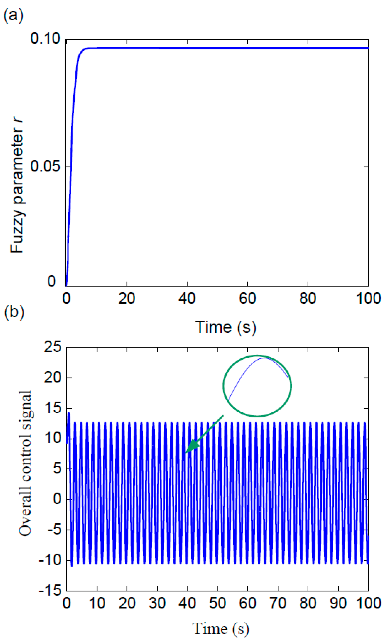
The presence of the fuzzy parameter r is a notable feature of the equation. Owing to the particularity of $\sum _{i=0}^6{\mu }_i=1$, the following equivalence can be obtained. Thus, it is possible to rewrite Equation (28) as follows.

$$u_{hit}={\displaystyle \sum _{i=0}^6{r}_i\cdot {\mu }_i\left(s\right)}=\left\{\begin{array}{c}r\cdot \theta \left(s\right)\hspace{1em}s>0\\ -r\cdot \theta \left(s\right)\hspace{1em}s<0\\ 0\hspace{1em}\hspace{1em}\hspace{1em}s=0\end{array}\right.$$

(30)

$\mathrm{with}\theta \left(s\right)={\mu }_1\left(s\right)+2{\mu }_2\left(s\right)+3{\mu }_3\left(s\right)$

Equation (30) revealed that sθ(s) > 0. By replacing u_hit in Equation (17) by Equation (30), time derivation of the sliding surface is rewritten as shown in Equation (31).

$$\dot{s}={\tilde{A}}^{T}B-g_{n}rs\theta \left(s\right)-L\left(t\right)$$

(31)

Thus, Equation (21) is rewritten as shown in Equation (32).

$$\dot{V}=-sL\left(t\right)-r{g}_{n}s\theta \left(s\right)\le -\left|s\right|\left(r{g}_n\left|\theta \left(s\right)\right|-\left|L\left(t\right)\right|\right)$$

(32)

To fulfill the requirement of the sliding condition of Equation (32), it is necessary for the fuzzy parameter r to meet the following condition in Equation (33).

$$r>\frac{\left|L\left(t\right)\right|}{g_n\left|\theta \left(s\right)\right|}$$

(33)

In the same manner as parameter vector A, a unique value (r^*) exists to obtain minimum control action, given as:

$$r^{*}=\frac{\left|L\left(t\right)\right|}{g_n\left|\theta \left(s\right)\right|}+\delta$$

(34)

where δ is a positive constant

Determining an exact value for r* in practical applications is often unattainable. Therefore, a straightforward adaptive algorithm is utilized to approximate the optimal value of r*. The controlling rule of the AFSMC is expressed as:

$$u=u_{eq}+u_{hit}=u_{eq}+\widehat{r}\theta \left(s\right)$$

(35)

In which $\widehat{r}$ is considered as the estimated value of the r^* optimal value.

By inserting Equation (15) into Equation (35), and then rearranging as shown in Equation (36) we obtain.

$$u=u_{eq}+u_h=\frac{1}{g_n}\left[{\stackrel{⃛}{x}}_{ref}-{\widehat{A}}^{T}B+2\lambda \ddot{e}+{\lambda }^2\dot{e}\right]+\widehat{r}\theta \left(s\right)$$

(36)

The dynamic of s is rewritten as:

$$\dot{s}=-A^{T}B+{\widehat{A}}^{T}B-g_n\widehat{r}\theta \left(s\right)-L\left(t\right)+g_n{r}^{*}\theta \left(s\right)-g_n{r}^{*}\theta \left(s\right)$$

(37)

Given $\tilde{r}=r^{*}-\widehat{r}$, Equation (37) is rearranged to obtain Equation (38).

$$\dot{s}={\tilde{A}}^{T}B+g_n\tilde{r}\theta \left(s\right)-L\left(t\right)-g_n{r}^{*}s\theta \left(s\right)$$

(38)

Currently, the Lyapunov candidate function is defined as:

$$V=\frac{1}{2}{s}^2+\frac{1}{2}{\tilde{A}}^T{Q}_A\tilde{A}+\frac{1}{2}{\delta }_2{\tilde{r}}^2$$

(39)

By differentiating V with respect to time and applying Equation (39), the following expression is obtained:

$$\dot{V}={\tilde{A}}^T\left(sB+Q_A\dot{\tilde{A}}\right)+\tilde{r}\left(s{g}_n\theta \left(s\right)+{\delta }_2\dot{\widehat{r}}\right)-s\theta \left(s\right)\left(\frac{L\left(t\right)}{\theta \left(s\right)}+g_n{r}^{*}\right)$$

(40)

and $\dot{\tilde{A}}$ = $\dot{\widehat{A}}$ and $\dot{\tilde{r}}$ = $-\dot{\widehat{r}}$, if the adaptive rules are designed as follows:

$$\begin{array}{l}\dot{\widehat{A}}=-{\delta }_1^{-1}sB\\ \dot{\widehat{r}}={\delta }_2^{-1}s{g}_n\theta \left(s\right)\end{array}$$

(41)

where δ₁ and δ₂ are the positive constants:

As sθ(s) > 0, by inserting Equation (41) into Equation (40) and then rearranging, Equation (40) can be expressed in the following form:

$$\dot{V}=-s\theta \left(s\right)\left(\frac{L\left(t\right)}{\theta \left(s\right)}+g_n{r}^{*}\right)\le \left|s\right|\left|\theta \left(s\right)\right|\left(\frac{\left|L\left(t\right)\right|}{\left|\theta \left(s\right)\right|}-g_n{r}^{*}\right)$$

(42)

By substituting Equation (34) into Equation (42), we simplify and obtain the convergence condition as in Equation (43).

$$\dot{V}\le -\left|s\right|\left|\theta \left(s\right)\right|\delta g_n\le 0$$

(43)

Consequently, in accordance with Lyapunov stability theory, the control system is deemed stable. Utilizing Barbalat’s lemma (Astrom and Wittenmark [39]), it can be inferred that the error will converge to zero.

4. Virtual Model and Simulation Result

4.1. Virtual Model

A virtual model of the EHA is developed using Amesim software to assess its control performance (Figure 4). The virtual model monitors the pressure at two ports of the hydraulic cylinder via two pressure sensors. Additionally, a position sensor measures the piston’s position, and the signal is sent to the controller for generating a control signal aimed at adjusting the speed of the servo motor. Subsequently, the virtual EHA model is integrated into the MATLAB/Simulink environment, where an adaptive fuzzy sliding mode controller is established, as shown in Figure 5. The EHA parameters required for this study are listed in

Table 1. Setting parameters for the EHA.

System’s Elements	Parameters	Values
Bidirectional pump	Maximum rotary speed	1000 (rpm)
	Oil volume per revolution	24 (cc/rev)
Hydraulic cylinder	Diameter of rod	10 (mm)
	Diameter of piston	20 (mm)
	Diameter of stroke	100 (mm)
	Dead volume at the ends	50 cm3
Hydraulic oil	Oil bulk modulus	1.5 × 109 (Pa)
	Oil specific gravity	0.87
Relief valve	Establishing pressure	50 (Pa)

.

4.2. Simulation Results

4.2.1. Case 1: Step Signal

The tracking mission involved achieving a desired position of 40 mm while under an external force of 1 kN. In this scenario, the external load was set at 100 kg, and a sampling time of 0.01 s was applied throughout the numerical simulation.

Figure 6 shows a comparison between the position performance of the EHA controlled by the conventional PID controller and the AFSMC. The PID controller’s parameters, including K_p = 0.43, K_i = 0.095, and K_d = 0.06, were selected using a trial-and-error method. While both controllers attained the desired low steady-state error, the PID controller demonstrated a significantly inferior response. The PID controller exhibited a peak overshoot of approximately 64 mm, unlike the AFSMC’s response, which was shown to be free of overshoot. Furthermore, the PID controller’s settling time was much longer than that of the AFSMC.

Increasing the load to 130 kg resulted in increased steady-state error for the PID controller, showing an oscillation phenomenon along the desired tracking trajectory as depicted in Figure 7. This was caused by the presence of the model nonlinearities and the dynamic uncertainties that resulted in reduced tracking efficacy of the PID controller. Thus, by using traditional PID, it would be very difficult to deal with these nonlinearity and uncertainty. However, knowing the exact model is not required in the proposed controller. These uncertain parameters can be lumped into the unknown function f(y₁, y₂, t), which is expressed approximately by Equation (7). The estimated value of this approximated function is illustrated in Figure 8, showing that the overall response of the proposed control remained almost unchanged.

4.2.2. Case 2: Multi-Step Signal

In this scenario, the multi-step response of the system under the control of both AFSMC and PID controllers would be examined. The system’s controller parameters remained constant while external load and force were set at 100 kg and 1 kN, respectively. Figure 9 shows the time history of the EHA’s position, with the reference value represented by the dashed line. The solid and dotted lines represent the control performance of the AFSMC and PID controllers, respectively. The PID controller’s tracking quality was seen to be significantly lower than that of the AFSMC controller due to nonlinearities. Initially, the position response of the controlled system was not optimal due to differences between the system’s initial state and the trajectory. However, after approximately 2 s, the proposed AFSMC controller was able to provide a highly accurate position response without substantial overshooting, while the PID controller’s tracking response only reached its steady state after 10 s and undergoes peak overshooting.

Furthermore, it was observed that the pressure, P₂, at the cylinder’s port 2 was nearly zero, and the pressure P₁ at port 1 was always greater than zero—remaining at 31.5 bar at steady-state, as shown in Figure 10. This was due to the oil flow from port 2 to port 1 through the hydraulic pump to create a positive pressure, overcoming the external load of 1 kN to extend from the initial position to a 50 mm position. However, when retracting to the 30 mm position, the external force caused the positive pressure P₁ to remain steady and exerts against the external load to maintain the system’s tracking ability.

4.2.3. Case 3: Sinusoidal Signal

In this case study, the tracking task involved a sinusoidal signal with a frequency of 0.1 Hz and amplitude of 30 mm. An external disturbance was also added as a sinusoidal force with a phase difference of 90° and the same frequency as the desired signal. This force has an amplitude of 1 kN (Figure 11). As the piston retracts, the external load transforms into a pulled force; conversely, when the piston extends, the external load becomes a pushed force. Consequently, at the two ends of the piston stroke, the load force becomes zero.

Figure 12 shows a comparison of the tracking response of the PID and AFSMC controllers. It can be seen that that the position response of the EHA controlled by the PID controller could not align with the reference, and the tracking error has increased significantly. Incorporating the AFSMC controller resulted in a smooth and close tracking of the reference, keeping the steady-state error within 1 mm. Moreover, at the initial stage, the piston can track the reference with great accuracy.

Figure 13 illustrates the pressure at the hydraulic cylinder’s two ports, showing the presence of disturbances resulting in a phase shift between the P₁ and P₂ pressures, resulting in P₁ > 0 and P₂ = 0 during piston extension. Conversely, the opposite holds when the piston retracts. The P₂ pressure is persistently greater than P₁ since chamber 2’s effective area is always smaller than that of chamber 1.

Figure 14 shows the continuous tuning of the fuzzy parameter of the auxiliary control law over time. After approximately 2.5 s, the fuzzy parameter of the auxiliary control law reaches its optimal estimation value of 0.147.

4.2.4. Case 4: Comparison between the Control Performance of the AFSMC and ASMC

A comparison was made between the AFSMC and the adaptive ASMC. The desirable trajectory for this comparison is a sinusoidal signal with an amplitude of 20 mm and a frequency of 0.5 Hz. The ASMC is determined by the equivalent control action equation (Equation (16)) and the auxiliary control action equation (Equation (17)). The adaptation law of the ASMC is calculated using Equation (22), while the hitting control gain of the auxiliary control action is set to η = 1.5. An external load with a sinusoidal form, having an amplitude of 1.1 kN and a frequency of 0.5 Hz, but with a phase difference of 90° compared to the desirable trajectory, is also applied.

The comparison in Figure 15 shows that the AFSMC and ASMC were able to follow the desired trajectories. However, the control performance of AFSMC was better than that of the ASMC. The tracking error of the AFSMC at the steady-state was within ±1.5 mm, while the position error of the ASMC (depicted by the dashed line in Figure 16) was greater (within ±10 mm). This was due to the hitting control gain of the ASMC being fixed at 1.5, resulting in a step signal of the auxiliary control action, as shown in Figure 17a. As a result, the control signal of the ASMC was not smooth (Figure 17b). The ASMC generated the chattering phenomenon, indicating that this controller provided a worse response than AFSMC.

To overcome this problem, the AFSMC has applied fuzzy sets to replace the hitting control law given by Equations (17) and (30). The result is a smooth curve of the fuzzy parameter, as shown in Figure 18a, with an optimal value of 0.94, indicating that the AFSMC can generate a smooth control signal, as shown in Figure 18b. This modification allowed the proposed AFSMC controller to provide a robust response with high accuracy by removing the chattering phenomenon. Additionally, the pressure variation at ports 1 and 2, shown in Figure 19, confirms that the pressure at port 2 is always larger than at port 1.

5. Conclusions

An adaptive fuzzy sliding mode controller (AFSMC) was successfully developed for the electro-hydraulic actuator (EHA) using mathematical modeling and virtual prototyping approaches. The controller structure incorporates two control actions, with one being equivalent and the other serving as an auxiliary control law. An approximate technique that combined basic functions was utilized to estimate the equivalent control action. Meanwhile, the hitting control action was determined through fuzzy logic techniques, leading to the complete removal of chattering phenomenon in the proposed controller. The parameters of the controller were adjusted through updated laws based on Lyapunov functions. The evaluation of EHA’s control performance were conducted through co-simulation using Amesim software to build the EHA virtual model, and Matlab/Simulink to create the controller. The EHA’s position response, controlled by AFSMC for input signals encompassing multi-step and sinusoids, has been obtained. The simulation results indicate that the AFSMC not only attained the desired position response, but also exhibited excellent stability and robustness as compared to PID and ASMC.

References

1. Sakai, S.; Maeshima, Y. A new method for parameter identification for N-DOF hydraulic robots. In Proceedings of the 2014 IEEE International Conference on Robotics and Automation (ICRA), Hong Kong, China, 31 May–7 June 2014; pp. 5983–5989. [Google Scholar]
2. Sakai, S.; Stramigioli, S. Visualization of hydraulic cylinder dynamics by a structure preserving nondimensionalization. IEEE/ASME Trans. Mechatron. 2018, 23, 2196–2206. [Google Scholar] [CrossRef] [Green Version]
3. Xia, Y.; Shi, Y.; Yuan, Y.; Zhang, Y.; Yao, Z. Analyzing of influencing factors on dynamic response characteristics of double closed-loop control digital hydraulic cylinder. J. Adv. Mech. Des. Syst. Manuf. 2019, 13, 48–64. [Google Scholar] [CrossRef] [Green Version]
4. Cundiff, J.S.; Kocher, M.F. Fluid Power Circuits and Controls: Fundamentals and Applications; CRC Press: Boca Raton, FL, USA, 2019. [Google Scholar]
5. Choi, J. Robust position control of Electro-Hydrostatic actuator systems with radial basis function neural networks. J. Adv. Mech. Des. Syst. Manuf. 2013, 7, 257–267. [Google Scholar] [CrossRef] [Green Version]
6. Altare, G.; Vacca, A. A design solution for efficient and compact electro-hydraulic actuators. Procedia Eng. 2015, 106, 8–16. [Google Scholar] [CrossRef] [Green Version]
7. Chen, M.; Zhao, D. The gravitational potential energy regeneration system with closed-circuit of boom of hydraulic excavator. Mech. Syst. Signal Process. 2017, 82, 178–192. [Google Scholar] [CrossRef]
8. Maré, J.-C.; Fu, J. Review on signal-by-wire and power-by-wire actuation for more electric aircraft. Chin. J. Aeronaut. 2017, 30, 857–870. [Google Scholar] [CrossRef]
9. Fu, Y.; Han, X.; Sepehri, N.; Zhou, G.; Fu, J.; Yu, L.; Yang, R. Design and performance analysis of position-based impedance control for an electrohydrostatic actuation system. Chin. J. Aeronaut. 2018, 31, 584–596. [Google Scholar] [CrossRef]
10. Electro-Hydraulic Actuators. Available online: https://power-packer.com/electro-hydraulic-actuators (accessed on 15 June 2019).
11. Kim, C.; Ro, P.I. A sliding mode controller for vehicle active suspension systems with non-linearities. Proc. Inst. Mech. Eng. Part D J. Automob. Eng. 1998, 212, 79–92. [Google Scholar] [CrossRef]
12. Huang, S.-J.; Chen, H.-Y. Adaptive sliding controller with self-tuning fuzzy compensation for vehicle suspension control. Mechatronics 2006, 16, 607–622. [Google Scholar] [CrossRef]
13. Cheng, G.; Shanan, Z. Adaptive time-varying sliding mode control for hydraulic servo system. In Proceedings of the ICARCV 2004 8th Control, Automation, Robotics and Vision Conference, Kunming, China, 6–9 December 2004; Volume 3, pp. 1774–1779. [Google Scholar]
14. Richardson, R.; Plummer, A.R.; Brown, M.D. Self-tuning control of a low-friction pneumatic actuator under the influence of gravity. IEEE Trans. Control Syst. Technol. 2001, 9, 330–334. [Google Scholar] [CrossRef]
15. Guan, C.; Pan, S. Adaptive sliding mode control of electro-hydraulic system with nonlinear unknown parameters. Control Eng. Pract. 2008, 16, 1275–1284. [Google Scholar] [CrossRef]
16. Acarman, T.; Hatipoglu, C.; Ozguner, U. A robust nonlinear controller design for a pneumatic actuator. In Proceedings of the 2001 American Control Conference (Cat. No.01CH37148), Arlington, VA, USA, 25–27 June 2001; Volume 6, pp. 4490–4495. [Google Scholar]
17. Xu, Z.-D.; Guo, Y.-Q. Fuzzy Control Method for Earthquake Mitigation Structures with Magnetorheological Dampers. J. Intell. Mater. Syst. Struct. 2006, 17, 871–881. [Google Scholar] [CrossRef]
18. Tang, C.; Yue, L.; Guo, L.; Zhou, S.; Zhou, W.; Wang, Z. Fuzzy Logic Control for Vehicle Suspension Systems. In Intelligent Robotics and Applications, Proceedings of the First International Conference ICIRA 2008, Wuhan, China, 15–17 October 2008; Xiong, C., Liu, H., Huang, Y., Xiong, Y., Eds.; Springer: Berlin/Heidelberg, Germany, 2008; pp. 197–206. [Google Scholar]
19. Chu, Z.; Xiang, X.; Zhu, D.; Luo, C.; Xie, D. Adaptive Fuzzy Sliding Mode Diving Control for Autonomous Underwater Vehicle with Input Constraint. Int. J. Fuzzy Syst. 2018, 20, 1460–1469. [Google Scholar] [CrossRef]
20. Razmi, H.; Afshinfar, S. Neural network-based adaptive sliding mode control design for position and attitude control of a quadrotor UAV. Aerosp. Sci. Technol. 2019, 91, 12–27. [Google Scholar] [CrossRef]
21. Zhao, T.; Chen, Y.; Dian, S.; Guo, R.; Li, S. General Type-2 Fuzzy Gain Scheduling PID Controller with Application to Power-Line Inspection Robots. Int. J. Fuzzy Syst. 2020, 22, 181–200. [Google Scholar] [CrossRef]
22. Phu, N.D.; Hung, N.N.; Ahmadian, A.; Senu, N. A New Fuzzy PID Control System Based on Fuzzy PID Controller and Fuzzy Control Process. Int. J. Fuzzy Syst. 2020, 22, 2163–2187. [Google Scholar] [CrossRef]
23. Ursu, I.; Tecuceanu, G.; Toader, A.; Calimoiu, C.; Ursu, F.; Berar, V. Neuro-fuzzy control synthesis for hydrostatic type servoactuators. Experimental results. INCAS Bull. 2009, 1, 136–150. [Google Scholar] [CrossRef]
24. Vukovic, M.; Murrenhoff, H. The Next Generation of Fluid Power Systems. Procedia Eng. 2015, 106, 2–7. [Google Scholar] [CrossRef]
25. Yordanov, S.; Ormandzhiev, K.; Mihalev, G. Comparative analysis of control quality between PI and FUZZY controller of experimental electrohydraulic servosystem. In Proceedings of the 2021 International Conference Automatics and Informatics (ICAI), Varna, Bulgaria, 30 September–2 October 2021; pp. 48–53. [Google Scholar]
26. Chen, G.; Liu, H.; Jia, P.; Qiu, G.; Yu, H.; Yan, G.; Ai, C.; Zhang, J. Position Output Adaptive Backstepping Control of Electro-Hydraulic Servo Closed-Pump Control System. Processes 2021, 9, 2209. [Google Scholar] [CrossRef]
27. Rybarczyk, D.; Milecki, A. The Use of a Model-Based Controller for Dynamics Improvement of the Hydraulic Drive with Proportional Valve and Synchronous Motor. Energies 2022, 15, 3111. [Google Scholar] [CrossRef]
28. Ren, G.; Mou, X.; Wen, X.; Chen, L. Position Control of a Single-Rod Electro-Hydrostatic Actuator Experiencing a Leaky Piston Seal. Math. Probl. Eng. 2022, 2022, 3166926. [Google Scholar] [CrossRef]
29. Sun, C.; Dong, X.; Wang, M.; Li, J. Sliding Mode Control of Electro-Hydraulic Position Servo System Based on Adaptive Reaching Law. Appl. Sci. 2022, 12, 6897. [Google Scholar] [CrossRef]
30. Park, H.-S.; Le, N.-T. Modeling and controlling the mobile harbour crane system with virtual prototyping technology. Int. J. Control Autom. Syst. 2012, 10, 1204–1214. [Google Scholar] [CrossRef]
31. Le, T.D.; Nguyen, P.T. Dynamic simulation of seat suspension system with virtual prototyping technology. J. Adv. Mech. Des. Syst. Manuf. 2017, 11, 56–66. [Google Scholar] [CrossRef] [Green Version]
32. Van, T.N.; Tran, H.Q.; Ha, V.X.; Ha, C.; Minh, P.H. Fuzzy Feedback Control for Electro-Hydraulic Actuators. Intell. Autom. Soft Comput. 2023, 36, 2441–2456. [Google Scholar]
33. Chen, Q.; Shao, H.; Liu, Y.; Xiao, Y.; Wang, N.; Shu, Q. Hydraulic-pressure-following control of an electronic hydraulic brake system based on a fuzzy proportional and integral controller. Eng. Appl. Comput. Fluid Mech. 2020, 14, 1228–1236. [Google Scholar] [CrossRef]
34. Chen, Q.; Sun, H.; Wang, N.; Niu, Z.; Wan, R. Sliding Mode Control of Hydraulic Pressure in Electro-Hydraulic Brake System Based on the Linearization of Higher-Order Model. Fluid Dyn. Mater. Process. 2020, 16, 513–524. [Google Scholar] [CrossRef]
35. Aly, A.A.; Elhabib, M.O.; Felemban, B.F.; Saleh, B.; Le, D.-N. Modeling and Simulation of Two Axes Gimbal Using Fuzzy Control. Comput. Mater. Contin. 2022, 72, 93–107. [Google Scholar] [CrossRef]
36. Kaliappan, P.; Ilangovan, A.; Muthusamy, S.; Sembanan, B. Temperature Control Design with Differential Evolution Based Improved Adaptive-Fuzzy-PID Techniques. Intell. Autom. Soft Comput. 2023, 36, 781–801. [Google Scholar] [CrossRef]
37. Tri, N.M.; Nam, D.N.C.; Park, H.G.; Ahn, K.K. Trajectory control of an electro hydraulic actuator using an iterative backstepping control scheme. Mechatronics 2015, 29, 96–102. [Google Scholar] [CrossRef]
38. Farrell, J.A.; Polycarpou, M.M. Adaptive Approximation Based Control: Unifying Neural, Fuzzy and Traditional Adaptive Approximation Approaches; John Wiley & Sons: Hoboken, NJ, USA, 2006. [Google Scholar]
39. Astrom, K.; Wittenmark, B. Adaptive Control, 2nd ed.; Addison-Wesley Publ. Co.: Boston, MA, USA, 1995. [Google Scholar]
Figure 1. A diagram illustrating the workings of an electro-hydraulic actuator [37].
Actuators 12 00258 g001
Figure 2. A graphical representation illustrating the controller’s composition based on the block diagram.
Actuators 12 00258 g002
Figure 3. The membership functions for the input variable s (a) and the output variable uhit (b).
Actuators 12 00258 g003
Figure 4. The development of the virtual model of the EHA utilizing Amesim software.
Actuators 12 00258 g004
Figure 5. The developed entire controlling scheme.
Actuators 12 00258 g005
Figure 6. Time response of the EHA for the external load of 100 kg.
Actuators 12 00258 g006
Figure 7. Time response of the EHA for the external load of 130 kg.
Actuators 12 00258 g007
Figure 8. The estimated value of f(y1, y2, t) versus time.
Actuators 12 00258 g008
Figure 9. System response with the AFSMC for multi-step input.
Actuators 12 00258 g009
Figure 10. The time history of pressure at port 1 (P1) and port 2 (P2) of cylinder with AFSMC for multi-step input.
Actuators 12 00258 g010
Figure 11. Load force versus time.
Actuators 12 00258 g011
Figure 12. Matching the location of the mass against both the actual and reference positions.
Actuators 12 00258 g012
Figure 13. The pressure condition at the hydraulic cylinder’s ports.
Actuators 12 00258 g013
Figure 14. Variation of fuzzy parameter.
Actuators 12 00258 g014
Figure 15. The time history of the position response of the system controller by the AFSMC and ASMC (notations for line types are expressed in the upper-right corner of the figure).
Actuators 12 00258 g015
Figure 16. The tracking error of the AFSMC and the ASMC (annotations of line types are presented in the upper-right corner of the figure).
Actuators 12 00258 g016
Figure 17. Auxiliary control signal (a) and overall control signal (b) for the ASMC.
Actuators 12 00258 g017
Figure 18. Variation of fuzzy parameter (a); overall control signal of the ASMC (b).
Actuators 12 00258 g018
Figure 19. Pressure variation versus time of system controlled by AFSMC (a) and ASMC (b).
Actuators 12 00258 g019