Article

Development of a Deformable Water-Mobile Robot

School of Mechatronics Engineering, Shenyang Aerospace University, Shenyang 110136, China
*
Author to whom correspondence should be addressed.
Actuators 2023, 12(5), 202; https://doi.org/10.3390/act12050202
Submission received: 13 April 2023 / Revised: 10 May 2023 / Accepted: 11 May 2023 / Published: 12 May 2023
(This article belongs to the Special Issue Modeling, Optimization and Control of Robotic Systems)

Abstract

:
This article proposes a deformable water-mobile robot that can be used for rescue work. The robot body adopts an open-motion chain structure with two degrees of freedom, including two drive modules and one main control module. The three modules are connected through deformation joints, and each drive module is equipped with an underwater thruster. The robot can obtain a triangle, linear shape, curved shape, and U-shape through deformation and have three types of motion: linear shape motion, U-shaped motion, and curved shape motion. In the linear shape, a multi-island genetic algorithm was used to optimize the structural parameters with the minimum resistance and the maximum volume. Floating state analysis was conducted in the U-shape, and the structural parameters were reasonably designed. By experimenting with the robot prototype on water, the robot can achieve oscillating, linear, U-shaped, and horizontal rotary motion, has an automatic adjustment function, and effective buoyancy meets the required requirements.

1. Introduction

The number of people killed due to water disasters has increased in recent years. It is vital to quickly reach the target location and successfully rescue people in the water. At present, manual rescue not only slows response time, but during the rescue of people in distress, due to the complexity and danger of the environment, the rescuers may have safety problems. Many companies and universities at home and abroad have researched water-mobile robots to meet the various needs of water work. With the comprehensive current research status, the water-mobile robot can be divided into traditional and non-traditional hull structures according to the structure. The traditional hull structure is mainly based on the common hull type modification, such as eVe-1 developed by Kim et al. This unmanned boat is a catamaran configuration [1]. Le developed a U-shaped unmanned boat based on the catamaran structure to perform water rescue missions [2]. Zong et al. developed a special trimaran based on the hull structure. This boat was fitted with T-shaped sails to improve sailing performance [3]. Goulon et al. developed an unmanned boat on the water called HARLE, equipped with a fisheries science echosounder for aquatic surveys [4]. Makhsoos et al. developed a water robot called Morvarid by using solar energy as a new source of energy [5]. Morge et al. developed a compact sailboat to take full advantage of wind energy, simplifying traditional sailboats’ structure and increasing flexibility [6]. Johnston et al. developed a wave-driven unmanned boat called AutoNaut, which can propel the body forward with alternating waves on the water [7,8]. For non-traditional hull structures, researchers from various countries have mainly used bionics to conduct relevant research [9,10,11,12,13]. Nad et al. developed a water robot consisting of four thrusters. This robot moves more flexibly [14]. Inoue et al. developed a robot called Quince. This robot has various detection devices to detect conditions such as body temperature [15]. Huang et al. developed a buoyancy-supported water strider robot based on the locomotor ability of water striders to achieve water walking capability [16].
The robots of Kim [1] and Zong [3] use a multi-hull structure for traditional hull structures. Such robots increase overall flexibility and stability but have a single structure and large size. The U-shaped unmanned boat developed by Le [2] can achieve rescue but has a high forward resistance due to its structure. Waterborne devices developed by Makhsoos [5], Morge [6], and Johnston [7,8] have been better developed in the energy direction. However, none of these studies proposed a suitable structure in terms of rescue. For non-hull structures, none of such bionic robots developed by Nad [14], Inoue [15], and Huang [16] have water rescue as their main application scenario.
For the above problems, a deformable water-mobile robot is designed in this paper [17]. This robot can reduce the resistance by deformation. The linear shape and U-shape of the robot are used as the main motion form. The robot was optimized by linear shape simulation and U-shaped floating state analysis to find the optimal size solution. Through experiments, it is verified that the deformable water-mobile robot can achieve the corresponding functions.

2. Robot Structure

2.1. Functional Requirements of Robots

According to the characteristics of the water rescue task, the robot needs to enter the working environment quickly and reach the target location quickly, and return safely after stably carrying the fallen person. As shown in Figure 1a, the robot designed in this article can be thrown directly into the water and enter the water environment smoothly. The robot is triangular when thrown, and the triangular structure is stable to resist the impact of falling water. As shown in Figure 1b, the robot can be unfolded into a linear form, which can quickly complete the adjustment of the upper and lower positions of the thrusters and quickly reach the target site. As shown in Figure 1c, the robot can take advantage of its structural characteristics to turn into a curved shape when turning, which can reduce the minimum turning radius. As shown in Figure 1d, the robot turns into a U-shape after reaching the target location and wraps the person up by differential steering to play the role of buoyancy support and return safely.

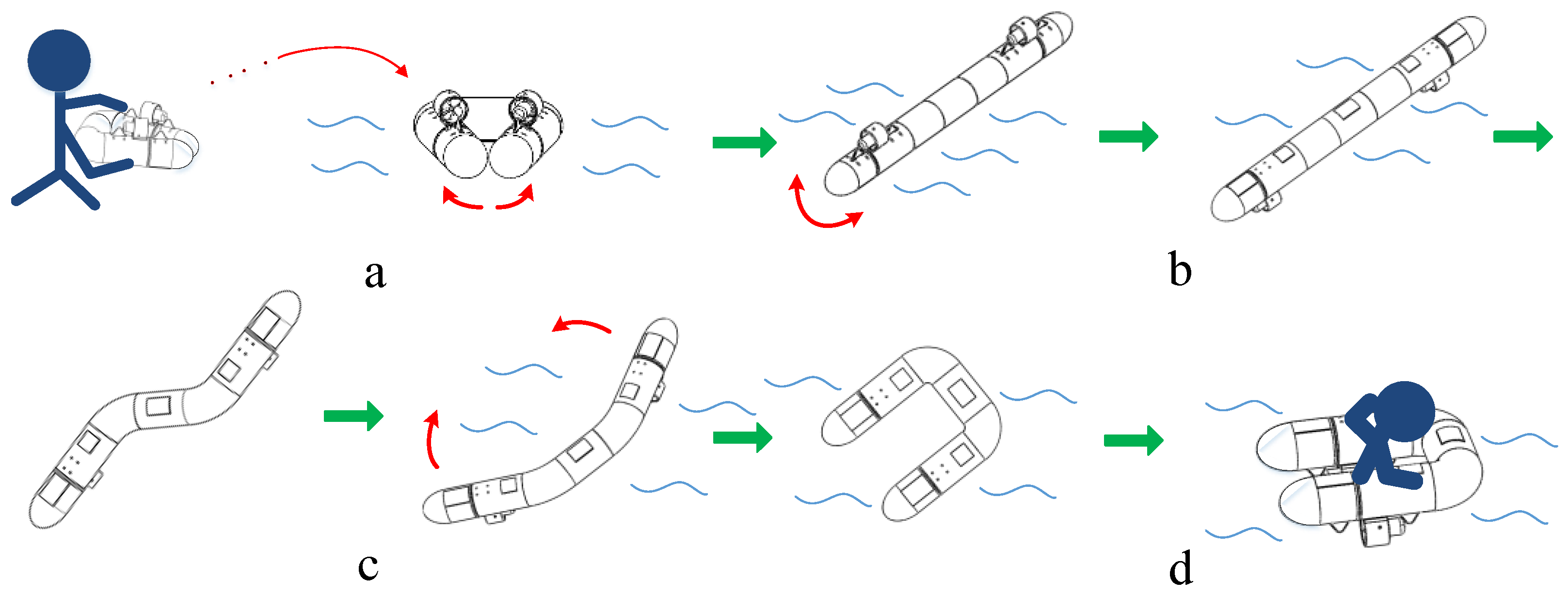
2.2. Principle of Configuration

In nature, water snakes are flexible and quick when swimming in water. They can bend their bodies to smoothly pass through various complex water environments, which is exactly the mobility characteristics needed for water-mobile robots. Based on the characteristics of biological water snakes, a new water-mobile robot with a three-link, two-drive joint open kinematic chain configuration was designed. The body includes a front segment (1), a middle segment (3), and a rear segment (4). The ends of the middle segment are connected to the front and rear segments by the deformable segment (2), respectively. The front and rear segments are fixed to the thruster (5). The schematic diagram and structural diagram of the mechanism are shown in Figure 2 and Figure 3.
Many current water-mobile robots with rescue aspects are U-shaped, as in reference [2], but the shape of such robots is immutable during movement. The robot in this article has a linear shape when it reaches the target location and a U-shape when it returns. Under the same structural parameters, the drag analysis is performed for the linear shape in this article and the U-shape in reference [2]. Water drag can be calculated as Equation (1) [18]:
F d = 1 2   ρ f   v d 2   A   C D
where Fd is the water drag, ρf is the density of water, vd is the robot’s speed, A is the cross-sectional area of the robot, and CD is the drag coefficient of the robot.
When the structural parameters of the two shapes are the same, assuming that the density of water and the robot’s speed is certain, the two shapes’ cross-sectional area and drag coefficient are obviously different. The cross-sectional area and drag coefficient of the linear shape are smaller than those of the U-shape, so the water drag in the linear shape will be smaller.

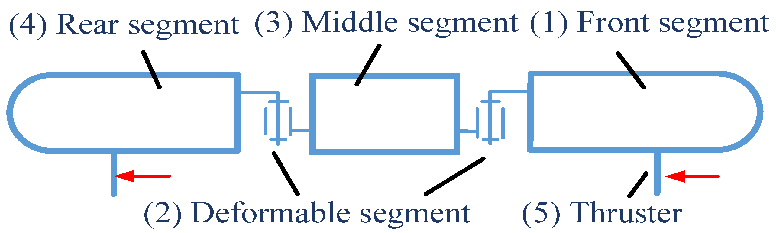
2.3. Structural Design of Robots

As shown in Figure 4, the middle segment includes a middle segment shell, with a middle hatch cover (9) set at the top of the middle segment shell, a middle segment sealed chamber (14) inside the middle segment shell, and line pipelines (10) set on both sides of the middle segment sealed chamber. The middle part of the middle segment sealed chamber is the controller chamber (13).
The deformable segment (2) includes a sealing tube (8), an upper base (17), a flanged shaft (18), a bearing (19), a coupling (21), a bracket (22), a steering gear (20), and a lower base (23). The sealing tube provides a sealing connection between the two rotating sub-joints. The flange shaft (18) is bolted to one end of the upper base (17) through its flange, and the outer circular surface of the shaft section of the flanged shaft is coaxially set with the bracket (22) through the bearing (19). The shaft section of the flange protrudes from the bearing section and is connected to the steering gear output shaft (20) by a coupling (21). The steering gear is bolted to one end of the lower base (23), the other end of the steering gear seat is hinged to the middle segment shell of the middle segment (3), and the steering gear (20) is connected to the controller via a wire.
The front segment of the body (1) has the same structure as the rear segment, including the segmented shell (11). A segmented hatch cover (7) is mounted on the segmented shell, and a segmented sealed chamber (6) is formed inside the segmented shell. The section of the segmented shell is shaped to resemble a rotary bullet. The segmented sealed chamber is divided into an electronic component chamber (15) and an embedded battery chamber (16), and the electronic component chamber is located near the middle segment (3). A battery is installed in the embedded battery chamber, and an electronic component chamber has a built-in electronic governor connecting the battery to the chassis thruster (5). The bottom of the segmented shell (11) has fins (12) and thruster mounts mounted by bolts, and the thruster mounts have chassis thrusters mounted on them. The two thrusters are propelled in the same direction.
Firstly, the staff threw the robot in a triangular state into the water. The staff presses the unfolding button, the front and rear segments of the body rotate in opposite directions, and both act simultaneously on the middle segment of the body to complete the unfolding action. After unfolding, it changes from a triangular state to a linear state when the front and rear segments’ chassis thrusters (5) are in the same line. After throwing in a triangular posture, the underwater thruster may be exposed to the air. As the robot becomes a linear shape, it is designed with an offset center of mass. Its special counterweight structure thrusters can be automatically submerged in the water to enter the movement preparation phase.
Based on the relative position of the robot and the target point, the robot chassis thruster (5) is controlled to drive rapidly in a linear state in the direction of the target point. If the robot drifts in the direction midway, the staff presses the adjustment lever of the controller to control the steering gear (20) at the deformable segment (2) to work. The steering gear drives the front segment and rear segment (4) to rotate so that the robot transforms into a curved shape for direction adjustment, thus changing the relative position of the two chassis thrusters in a non-linear state, and the two chassis thrusters do not share the same thrust direction to achieve the purpose of motion steering.
After reaching the target point, the staff presses the U-shaped button of the operator, and the steering gear at the deformable segment works and drives the front and rear segments to rotate, deforming the robot into a U-shaped state. Currently, the front and rear segments are in a non-collinear parallel state of the chassis thrusters for the differential motion to achieve the robot’s attitude adjustment to avoid directional drift until the stable return to the safety zone.

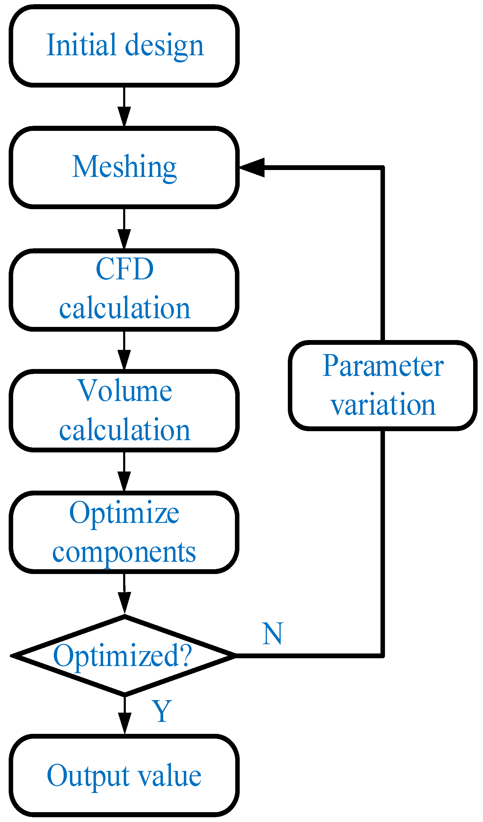
3. Shape Optimization Analysis

3.1. Force Analysis

In this article, the force analysis of the robot is performed while in the manned state. Due to the presence of the human itself discharging the volume of water, the buoyancy force of the water to the human is F1. The robot discharges the volume of water, the buoyancy force of the water to the robot is F2, m1g is the weight of the human, and m2g is the weight of the robot, as shown in Figure 5.
Buoyancy can be calculated as Equation (2):
Ff = ρf g Vf
where Ff is the robot’s buoyancy, g is gravity’s acceleration, and Vf is the volume of discharged water.
People on the water can displace about 80–90% of their volume. This article is designed to be able to rescue 75 kg adults as the goal, excluding the buoyancy of the human displacement volume. The load-bearing weight is reduced by about eight times. The robot requires a minimum effective load-bearing volume of about 0.0019 m3 and an effective load-bearing capacity of 1.9 kg.

3.2. Fluid Dynamics Control Equations and Turbulence Models

When a robot moves in the water environment, the fluid as a continuous medium should follow three major laws: the law of conservation of mass, conservation of momentum, and conservation of energy. This article develops the mathematical model using the CFD method [19]. People for hydrodynamic analysis are usually assumed to be incompressible, so only consider satisfying the mass and momentum conservation equations.
Menter optimized using the standard k-ω model and proposed the SST k-ω turbulence model. The SST k-ω turbulence model has higher accuracy and credibility, so the SST k-ω turbulence model is chosen as the CFD numerical simulation calculation model in this article. The control equations for the SST k-ω turbulence models are presented in the literature [19].

3.3. Determination of Objective Function and Constraint Conditions

Because the robot designed in this article is a three-segment robot, to ensure the overall stability of the robot, the bow and stern adopt a consistent external structure. Huapan et al. [20] showed that the sailing drag of semi-ellipsoid and semi-ellipse is less, so the bow and stern both use the semi-ellipsoid structure, and the linear shape control parameters are shown in Figure 6.
The equation of the curve of the semi-ellipse can be calculated as Equation (3) [20]:
y = ± d 2 a a 2 x 2
The volume of the body can be calculated as Equation (4):
V = π d 2 a 3 + d 4
where d is the maximum cross-sectional diameter, b is the length of the middle section of the body, a is the length of the semi-ellipse, and x is the distance from the point on the long axis to the vertex of the ellipse.
In this article, a rectangular computational domain of 4 m × 2 m × 2 m is established with the middle of the robot as the origin, a dense grid is used near the surface of the robot, and the final grid number of the whole basin is about 1 million cells. To make the robot move at a speed of 0.7 m/s when the size structure is optimal, set the water flow velocity for this speed for the robot drag simulation calculation. The fluid medium is set to liquid water and air, the inlet condition of the flow field is set to velocity inflow, the outlet is pressure outlet, and both the robot surface and the flow field boundary are set to a stationary wall with zero roughness.
In this article, the robot’s size is optimized to improve the robot’s overall performance. On the one hand, the optimization makes the robot as large as possible, which generates more buoyancy and leaves more space to carry various electronic devices. On the other hand, it makes the drag force as small as possible to achieve an energy-efficient design. In this article, to meet the robot’s functional requirements to prevent the control parameters from being too small or too large and leading to an unreasonable design, the relevant dimensions should be limited to determine the upper and lower limits of each parameter. The optimization objectives, as well as the constraints, are as follows:
Objective Minimize : Drag Maximize : Volume
Constraints 45 a 135 750 b 1200 50 d 275

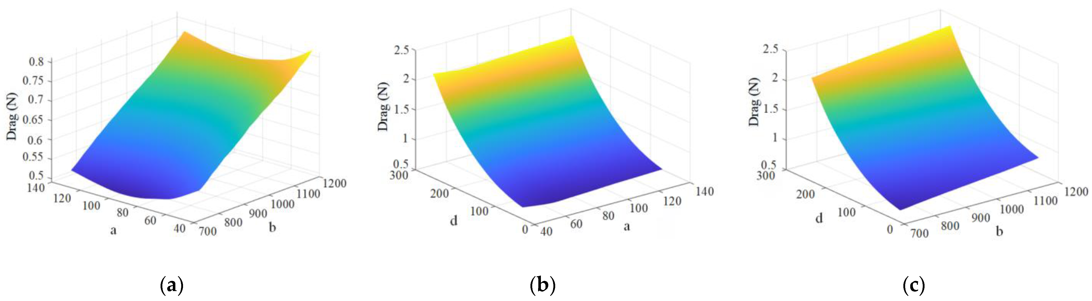
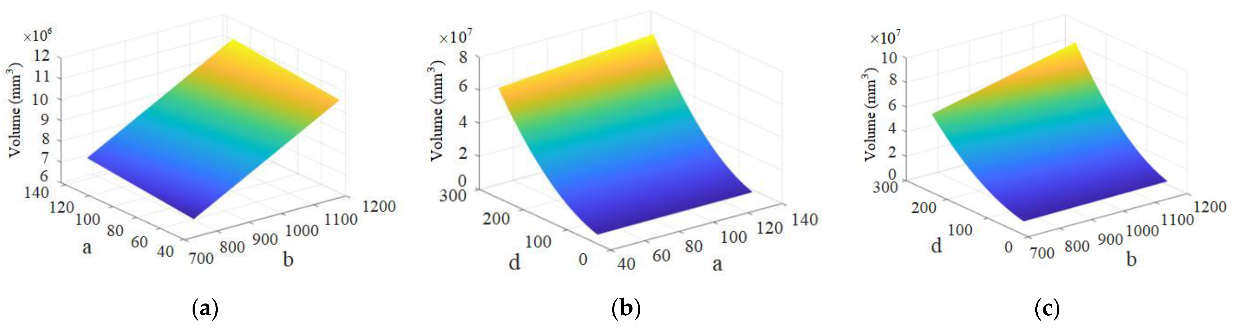
3.4. Simulation Analysis

Under the constraint of the feasible domain, the 3D surface plots of the independent and dependent variables (drag) are derived using Matlab simulation software. The interrelationships between the respective independent and dependent variables are obtained, as shown in Figure 7. Figure 7a represents the surface plot of the relationship between the independent variables a and b and the drag when d = 90. Figure 7b represents the surface plot of the relationship between the independent variables a and d and the drag when b = 1000. Figure 7c represents the surface plot of the relationship between the independent variables b and d and the drag when a = 25.
The figure above shows the size of the three parameters a, b, and d directly affecting drag. The change in the value of d has a significantly larger effect on the drag value than the change in the values of a and b. The range of d variation is the most sensitive to the effect of drag.
With the objective function equation of volume above, the 3D surface plots of the independent and dependent variables (volume) are simulated using Matlab simulation software under the constraint range. Figure 8a represents the surface plot of the relationship between the independent variables a and b and the volume when d = 90. Figure 8b represents the surface plot of the independent variables a and d versus volume when b = 1000. Figure 8c represents the surface plot of the independent variables b and d versus volume when a = 125.
The figure above shows the size of the three parameters a, b, and d directly affecting the volume. The changes in the values of b and d have a significantly larger effect on the volume taken than the value of a. It can be seen in Figure 8c that when the value of d is small, the change in the value of b does not have a significant effect on the volume. As the value of d increases, the value of b becomes more influential on the volume. The degree of effect of d is larger than that of b. The range of variation of d is most sensitive to the volume effect.
According to the above objective function and constraints, the volume maximum and drag minimum are simultaneously used as optimization objectives to find the optimal solution. The optimization design platform is established, and the optimization flow chart is shown in Figure 9. First, set the initial values of the 3D model control parameters. The initial values of each parameter are set as follows: a = 90, b = 1000, and d = 100. The model is then meshed, and the drag and volume values are calculated. The optimization component is then used to regenerate the control parameter values based on the obtained drag and volume and repeat the above steps until the optimal solution is found.
Optimization is performed according to the parameters given above. The values of the parameters are continuously changed in the optimization, and the drag values obtained from the iterative calculations are extracted. In this article, a multi-island genetic algorithm is chosen as the optimization method to find the optimal solution and avoid getting a locally optimal solution [21,22,23]. The population size of the genetic algorithm is chosen as 10, the number of evolutionary generations is 10, the crossover probability is 1, the variation probability is 0.01, and the migration probability is 0.01, which is calculated 1000 times. The feasible solutions for volume and drag are shown in Figure 10:
The above figure shows the calculation results obtained with the minimum drag and the maximum volume simultaneously as the optimization objectives. For a robot to increase its volume, it must reduce some of its drag. Similarly, if a robot profile with optimal drag performance is sought, then the requirement for a volumetric target needs to be reduced. No matter how the shape of the rotary body changes at a certain volume value, it will not be less than a certain drag value. The minimum drag value increases approximately linearly with the volume increase. Based on the required volume size of the robot, select the optimized values for the combination of design parameters as shown in Table 1:
The above table shows that the volume of the initial design is 8,796,459 mm3, the drag is 0.512 N, the optimized volume is 8,956,102 mm3, and the drag is 0.455 N. The optimized water-mobile robot has 11.1% less drag and 1.8% more volume. As shown in Figure 11, the wave generated by the initial size and the optimized size are shown.
As can be seen from the figure, the waves generated around the optimized size are significantly smaller than the initial size, and the wave height is reduced by 16.7%. The optimized wave amplitude of the body likewise reflects the effective improvement of the body drag [24].

4. U-Shaped Floating State Analysis

The robot needs to become U-shaped when it reaches the target location, and this form structure is less prone to tipping and has a larger lateral moment of inertia [25]. The U-shaped body size has a great effect on its smoothness. Angular tilt occurs when the forces on the left and right sides of the lateral and longitudinal surfaces are not balanced. Reasonable design of the left and right module spacing can balance the lateral and longitudinal smoothness. Analyze the impact of the movement of small-weight objects on the small tilt angles on both sides separately. As shown in Figure 12, the shape control parameters of this shape include lateral spacing k1 and longitudinal spacing k2.

4.1. Center of Gravity Calculation

In the linear shape, the coordinate system is established with the midpoint at the bottom of the robot’s midsection as the origin O, the direction pointing to the thruster as the X-axis, the vertical direction as the Z-axis, and the Y-axis perpendicular to the XOZ plane as shown in Figure 13.
In the U-shape, the coordinate system is established with the midpoint at the bottom of the robot’s midsection as the origin O, the direction pointing to the thruster as the Y-axis, the vertical direction as the Z-axis, and the X-axis perpendicular to the YOZ surface as shown in Figure 14.
Each part of the robot is in the O-XYZ coordinate system. The mass of the robot is W and contains n masses. The mass point’s mass is mi, and the position of each mass point is (xi,yi,zi). The position of the center of gravity can be calculated as Equations (7)–(9):
x G = i = 1 n m i   x i W
y G = i = 1 n m i   y i W
z G = i = 1 n m i   z i W
When the robot is in the linear shape state, the center of gravity coordinates of the robot is (0, 0, 37.4). In the U-shaped state, the coordinates of the robot’s center of gravity are (0, K, 37.4), and K is the value associated with k1.

4.2. Buoyancy Center Calculation

The derivation process of the buoyancy center calculation is in Appendix A. When the robot is in a linear shape, the X and Y directions are symmetrical, so x = 0 and y = 0, and the buoyancy center coordinates are (0, 0, 21.3). In the U-shaped state, the x-direction is symmetric with x = 0, and the buoyancy center coordinates are (0, K, 21.3). The center of gravity position is higher than the buoyancy center position in both linear shape state and U-shaped state.

4.3. Floating State Analysis

The tilt angle resulting from the weight movement is influenced by the parameters k1 and k2 in the lateral and longitudinal plane, respectively. Since the total length of the body remains unchanged, the two parameters are related by the following Equation, and at this time, the control parameter is only one variable, k1.
k1 + 2k2 = 1412
When in the lateral plane, move the p-weight object from point A to point A1 along the lateral horizontal direction. As shown in Figure 15, the robot’s center of gravity moves from the original point GH0 to point GH1. The body produces a lateral tilt, and the waterline moves from W0L0 to W1L1.
After the object moves, the robot will have a lateral angle tilt, and the derivation process is shown in Appendix B.
At the longitudinal plane, the p-weight object is moved from point B to point B1 along the longitudinal horizontal direction, as shown in Figure 16.
After the object is moved, the robot will have a longitudinal angle tilt, and the derivation process is shown in Appendix C.
When the p-weight object is 0.3 kg, the image of k1 against the lateral tilt angle α and the longitudinal tilt angle β is obtained, as shown in Figure 17.
The above figure shows that when the moving weight is certain, with the increase of k1, the overall tendency of the lateral tilt angle decreases, and the overall tendency of the longitudinal tilt angle increases. When k1 is about 0.5 mm, the two curves cross, and the lateral and longitudinal inclination angles are equal. When k1 is less than 0.5 mm, the trend of decreasing the lateral tilt angle is more drastic, and the longitudinal tilt angle also shows a slow decreasing trend. When k1 is larger than 0.5 mm, the decreasing lateral tilt angle trend is more moderate, and the increasing longitudinal tilt angle trend is more drastic. Considering the actual needs, the final choice of k1 is 0.4 mm.

5. Robot Prototype Experiment

5.1. Robot Prototype

In this article, platform test experiments of the robot were conducted on the water to verify the effectiveness of the robot prototype functions based on whether the robot can achieve the corresponding motion by experimenting with the effective load-carrying capacity, the automatic adjustment function, and different motion states. The model number of the remote control is FOSS FS-i6, the model number of the receiver is FS-iA6, the model number of the thruster is T60, the model number of the electronic governor is SHARK-50A, the model number of the servo is S9177SV, and the model number of the gyroscope angle sensor is WT901WIFI. The technical data of the experimental prototype are shown in Table 2, and the schematic diagram of each attitude of the solid prototype after assembly is shown in Figure 18.

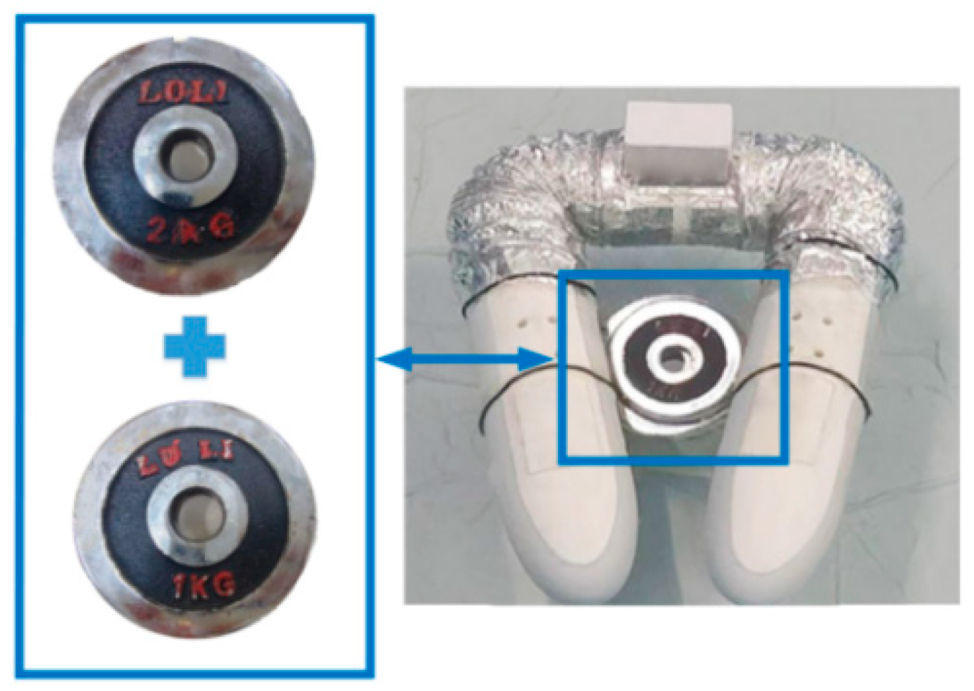
5.2. Bearing Capacity Test Experiment

Experiment on the effective load-carrying capacity of the experimental robot prototype. When the robot is in U-shape, the dumbbell piece is used to simulate the actual weight, and the weight is bound to the front and rear segments to imitate the human arm, and this state can enclose the weight and play the role of buoyancy support. When the weight is 3 kg, the horizontal surface reaches the state shown in Figure 19, and the robot is about to miss the horizontal surface. The robot sinks underwater when the weight is added to 4 kg. The effective load-carrying capacity is 3–4 kg, which meets the initial performance index requirements.

5.3. Robot-Throwing Expansion Experiment

The staff threw the robot in the triangle state into the water and pressed the button of the handheld operator to convert the triangle into a linear shape. The front and rear segments of the body rotate in opposite directions, and the middle segment of the body is relatively fixed to complete the unfolding experiment, as shown in Figure 20.

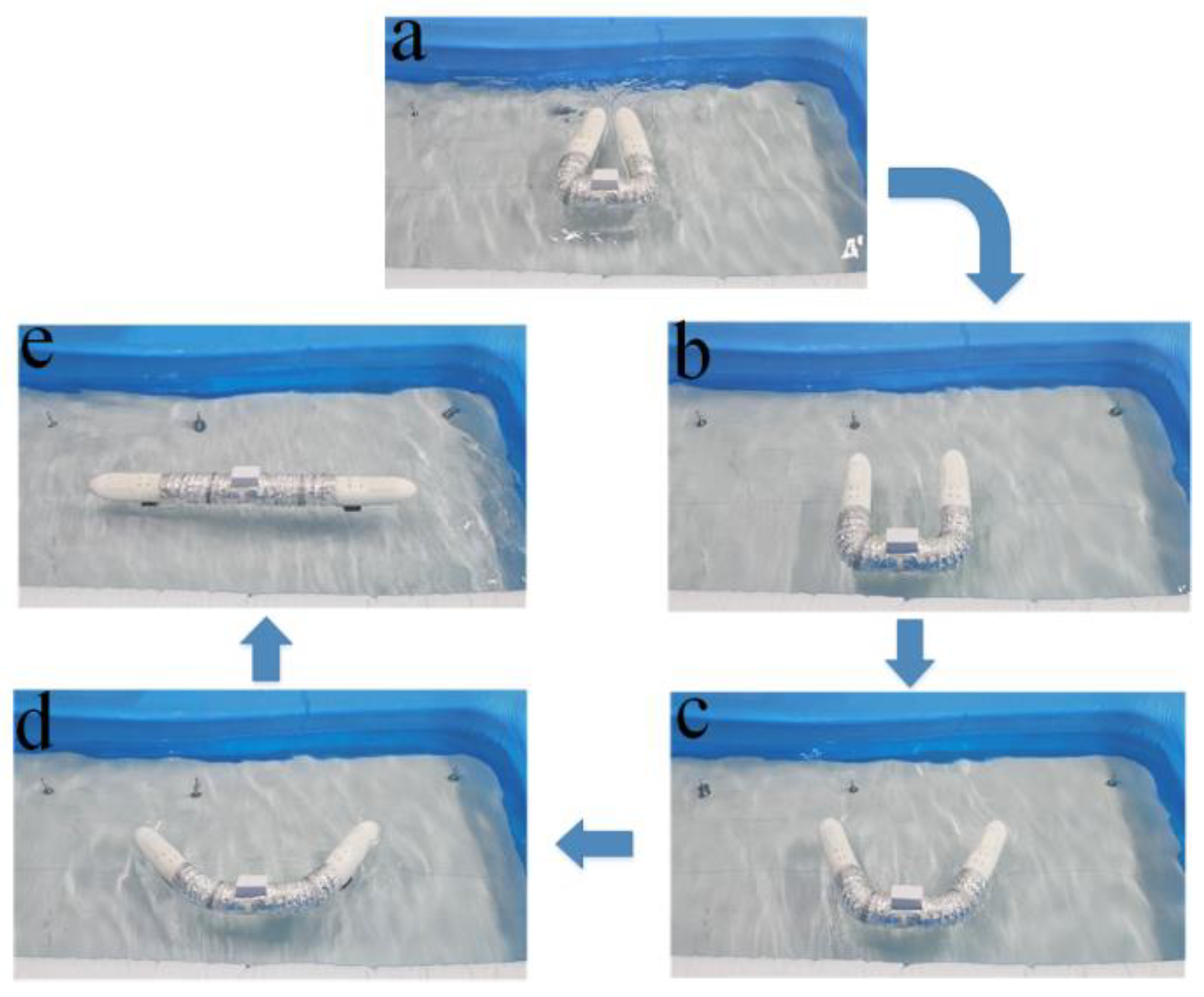
5.4. Automatic Attitude Adjustment Experiment

Since the robot can be thrown to the surface at will, it is important to ensure that the robot can automatically adjust so that the thrusters remain underwater. During the adjustment process, when the robot is tilted at a certain angle, a recovery torque is generated to return the robot to a positive floating state. The vertical submerged state of the thruster is set to 0°, and the vertical exposure of the thruster to air is set to −180°. Theoretically, the recovery torque is 0 for robot tilt angles of 0° and −180°. Experimentation on the functional prototype of the robot when the thruster is −180°. The effect is shown in Figure 21A, and the real-time data of the robot tilt angle is shown in Figure 21B.
When the tilt angle is −180°, the recovery moment is 0. However, in the actual situation, the left and right forces of the robot on the water surface cannot be perfectly balanced. As shown above, the thrusters can be automatically submerged in real situations.

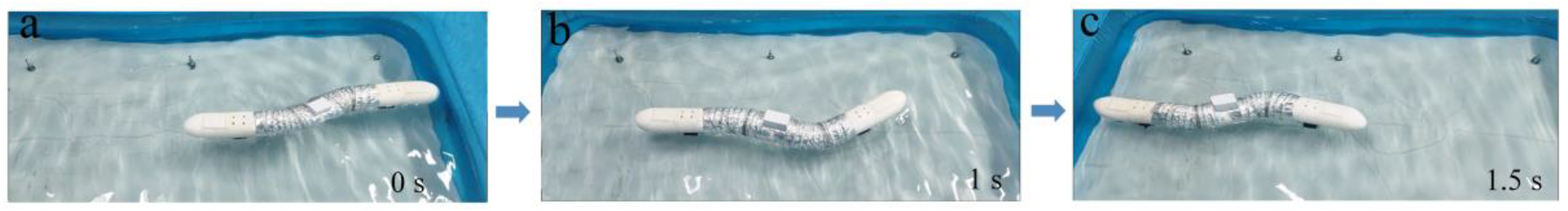
5.5. Oscillating Motion Experiment

Due to the special structural form of robots, they can rely on their own structural characteristics for swinging motion. Figure 22 shows the motion of the robot in the swing state. The remote control controls the steering gear to make the rear segment swing from 0 to 40°. The robot moves flexibly during the swing state and has low motion noise.

5.6. Direct Flight Motion Test

Conduct experiments on linear-shaped and U-shaped direct sailing movements on the water. Only longitudinal thrust is applied to the robot to ensure straight navigation of the robot, and the ground angle is put in the pool as a position reference. Figure 23 shows the direct sailing movements state of the robot.
The robot starts from a standstill, and observing the position of the reference object and the robot shows that the motion trajectory is straight, which indicates that the robot has a good stability of motion posture on the water surface.

5.7. Horizontal Rotary Motion Experiment

In the U-shape, the rotation speed of the left and right propellers is adjusted so there is a certain difference in their output power, and the robot will appear to steer, as shown in Figure 24A. When the remote control controls the steering gear at the deformable section of the robot, the front and back segments swing opposite to 55° and turn into a curved shape. Under the action of the thruster, the motion trajectory is also horizontal rotary, as shown in Figure 24B.
In the U-shape, the robot can achieve slewing motion under the action of thrust and bow moment when there is a certain deviation between the left and right propeller speed. In the U-shape, when the propeller speed is the same, and the output power is equal, the robot can also achieve rotary motion, which aligns with the general rule of horizontal rotary motion of water-mobile robots.

6. Conclusions

A deformable water-mobile robot is proposed for the specific needs of water rescue equipment. The robot has a two-degree-of-freedom chain structure that can be deformed to respond to different work requirements. The robot has a two-degrees-of-freedom chain structure that can be deformed to respond to different work requirements. Compared with the traditional U-shaped water-mobile robot, this robot can quickly reach the target location by morphing into a linear shape. An optimization design platform is established in linear shape to optimize the robot’s shape parameters based on a multi-island genetic algorithm with the objectives of minimum drag and maximum volume. Additionally, the floating state analysis was carried out in U-shaped to get the best shape structure. Finally, the robot prototype was experimented on the water surface. The robot’s effective load-carrying capacity meets the design requirements and can be deployed smoothly after throwing. The thruster can automatically sink underwater according to its adjustment function, which is better for achieving different movement functions. A deformable water-mobile robot is proposed to solve the current life-saving equipment structure of a single, large water drag and other shortcomings. Subsequently, it is necessary to introduce dynamics models, add precise control systems, and cooperate with vision and other systems for autonomous navigation control.

Author Contributions

Conceptualization, C.Y.; methodology, all authors.; software, Y.S.; validation, S.Y. and Y.W.; formal analysis, Y.S.; investigation, S.Y.; resources, C.Y.; data curation, Y.W.; writing—original draft preparation, Y.S.; writing—review and editing, S.Y.; visualization, Y.W.; supervision, C.Y.; project administration, C.Y.; funding acquisition, C.Y. All authors have read and agreed to the published version of the manuscript.

Funding

Liaoning Provincial Natural Science Foundation, grant number: 20180520033. Tundamental research funds for National Natural Science Foundation of China: 52005349. Liaoning Provincial Education Department Fund-“Seedling Raising” Project for Young Scientific and Technological Talents: JYT2020136.

Data Availability Statement

Not applicable.

Conflicts of Interest

The authors declare no conflict of interest.

Appendix A

This article uses the segmentation method to calculate the position coordinates of the robot’s buoyancy center. Parallel to the coordinate plane YOZ, a thin slice is taken in part below the draft line, and its thin microvolume can be calculated as Equation (A1):
dVf = Asdx
The static moment of the thin film microvolume to the coordinate plane can be calculated as Equations (A2)–(A4):
dMyoz = xa As dx
dMxoz = ya As dx
dMyox = za As dx
The coordinates of the center of buoyancy can be calculated as Equations (A5)–(A7):
x B = M yoz V f
y B = M xoz V f
z B = M yox V f

Appendix B

When the object moves, the robot tilts at a lateral angle. The buoyancy center BH0 will make a circular motion with the point of steady center MH as the center and the radius HBM as the steady lateral center. The lateral stability center radius HBM can be calculated as Equation (A8) [26]:
H BM = I H V f
where IH is the lateral moment of inertia.
The high HGM of lateral stability in this state can be calculated as Equation (A9):
H GM =   H BM   H BG
The cross-tilt angle α of the robot after the lateral movement of the weight p can be calculated as Equation (A10):
α   =   arctan p   k 1 H GM
where Δ is the discharge volume.

Appendix C

When the object moves, the robot tilts at a longitudinal angle. The longitudinal stability center radius ZBM can be calculated as Equation (A11) [26]:
Z BM = I Z A W   x f 2 V f
where IZ is the longitudinal moment of inertia, AW is the waterline surface area at Z from the base plane, and xf is the longitudinal coordinate of the waterline surface area AW shape center at Z from the base plane.
The high ZGM of longitudinal stability can be calculated as Equation (A12):
Z GM =   Z BM   Z BG
The longitudinal inclination angle β of the robot after the longitudinal movement of the weight p can be calculated as Equation (A13):
β   =   arctan p   1412 k 1 2     Z GM

References

  1. Kim, T.; Choi, J.; Lee, Y.; Choi, H.-T. Development of a Multi-Purpose Unmanned Surface Vehicle and Simulation Comparison of Path Tracking Methods. In Proceedings of the 2016 13th International Conference on Ubiquitous Robots and Ambient Intelligence (URAI), Xi’an, China, 19–22 August 2016; pp. 447–451. [Google Scholar]
  2. Le, Y. Research on Waterjet Propulsion and Navigation Control of Unmanned Vehicles. Master’s Thesis, Zhejiang University, Hangzhou, China, 2019. [Google Scholar]
  3. Zong, Z.; Sun, Y.; Jiang, Y. Experimental Study of Controlled T-Foil for Vertical Acceleration Reduction of a Trimaran. J. Mar. Sci. Technol. 2019, 24, 553–564. [Google Scholar] [CrossRef]
  4. Goulon, C.; Le Meaux, O.; Vincent-Falquet, R.; Guillard, J. Hydroacoustic Autonomous Boat for Remote Fish Detection in LakE (HARLE), an Unmanned Autonomous Surface Vehicle to Monitor Fish Populations in Lakes. Limnol. Oceanogr. Methods 2021, 19, 280–292. [Google Scholar] [CrossRef]
  5. Makhsoos, A.; Mousazadeh, H.; Mohtasebi, S.S.; Abdollahzadeh, M.; Jafarbiglu, H.; Omrani, E.; Salmani, Y.; Kiapey, A. Design, Simulation and Experimental Evaluation of Energy System for an Unmanned Surface Vehicle. Energy 2018, 148, 362–372. [Google Scholar] [CrossRef]
  6. Morge, A.; Pelle, V.; Wan, J.; Jaulin, L. Experimental Studies of Autonomous Sailing with a Radio Controlled Sailboat. IEEE Access 2022, 10, 134164–134171. [Google Scholar] [CrossRef]
  7. Johnston, P.; Pierpoint, C. Deployment of a Passive Acoustic Monitoring (PAM) Array from the AutoNaut Wave-Propelled Unmanned Surface Vessel (USV). In Proceedings of the OCEANS 2017, Aberdeen, UK, 19–22 June 2017; pp. 1–4. [Google Scholar]
  8. Poole, M.; Johnston, P. Autonomous surveying of shallow coastal waters for clean seas and shorelines: Coastal monitoring of water quality. Hydro Int. 2017, 21, 24–27. [Google Scholar]
  9. Wang, K.; Ma, Y.; Shan, H.; Ma, S. A Snake-Like Robot with Envelope Wheels and Obstacle-Aided Gaits. Appl. Sci. 2019, 9, 3749. [Google Scholar] [CrossRef]
  10. Nguyen, Q.V.; Chan, W.L. Development and flight performance of a biologically-inspired tailless flapping-wing micro air vehicle with wing stroke plane modulation. Bioinspir. Biomim. 2018, 14, 016015. [Google Scholar] [CrossRef] [PubMed]
  11. Picardi, G.; Laschi, C.; Calisti, M. Model-Based Open Loop Control of a Multigait Legged Underwater Robot. Mechatronics 2018, 55, 162–170. [Google Scholar] [CrossRef]
  12. Yang, W.; Zhang, W. A Worm-Inspired Robot Flexibly Steering on Horizontal and Vertical Surfaces. Appl. Sci. 2019, 9, 2168. [Google Scholar] [CrossRef]
  13. Yan, J.; Yang, K.; Liu, G.; Zhao, J. Flexible driving mechanism inspired water strider robot walking on water surface. IEEE Access 2020, 8, 89643–89654. [Google Scholar] [CrossRef]
  14. Nađ, Đ.; Mišković, N.; Mandić, F. Navigation, Guidance and Control of an Overactuated Marine Surface Vehicle. Annu. Rev. Control. 2015, 40, 172–181. [Google Scholar] [CrossRef]
  15. Inoue, T.; Shiosawa, T.; Takagi, K. Dynamic Analysis of Motion of Crawler-Type Remotely Operated Vehicles. IEEE J. Ocean. Eng. 2013, 38, 375–382. [Google Scholar] [CrossRef]
  16. Huang, H.; Sheng, C.; Wu, G.; Shen, Y.; Wang, H. Stroke Kinematics Analysis and Hydrodynamic Modeling of a Buoyancy-Supported Water Strider Robot. Appl. Sci. 2020, 10, 6300. [Google Scholar] [CrossRef]
  17. Changlong, Y.; Rui, W.; Yingxin, S.; Bing, W.; Biao, T.; Borui, Z.; Linglong, G.; Jiaqi, F. A Snake-Like Surface Rescue Robot and Its Control Method. CN Patent 111874185 A, 2 February 2022. [Google Scholar]
  18. Wang, M.; Tian, Y.; Yang, S.; Wang, P. Study on the Calculation Method of Water Inflow Velocity of Loose Rock Landslide. Sustainability 2022, 14, 12767. [Google Scholar] [CrossRef]
  19. Anderson, J.D. Basic Methods of computational fluid dynamics. In Fundamentals and Applications of Computational Fluid Dynamics, 1st ed.; Songping, W., Zhaomiao, L., Eds.; Machinery Industry Press: Beijing China, 2019; pp. 149–193. [Google Scholar]
  20. Huapan, X.; Zifan, F.; Chen, Z.; Kongde, H.; Weihua, Y.; Hongzhu, D. Research on structural resistance characteristics of underwater streamline body and its application. J. Three Gorges Univ. 2013, 35, 92–96. [Google Scholar]
  21. Song, B.; Lyu, D.; Jiang, J. Optimization of Composite Ring Stiffened Cylindrical Hulls for Unmanned Underwater Vehicles Using Multi-Island Genetic Algorithm. J. Reinf. Plast. Compos. 2018, 37, 668–684. [Google Scholar] [CrossRef]
  22. Pang, Y.; Wamg, Y.; Yang, Z.; Gao, T. Myring type rotary hull direct sailing drag calculation and boat type optimization. J. Harbin Eng. Univ. 2014, 35, 1093–1098. [Google Scholar]
  23. Peng, D. Research on Multi-Objective Optimal Design of Three-Body Combined Autonomous Underwater Vehicle Based on Parameterization. Master’s Thesis, South China University of Technology, Guangzhou, China, 2020. [Google Scholar]
  24. Cheng, X.; Feng, B.; Liu, Z.; Chang, H. Hull Surface Modification for Ship Resistance Performance Optimization Based on Delaunay Triangulation. Ocean. Eng. 2018, 153, 333–344. [Google Scholar] [CrossRef]
  25. Zhang, W.; Li, Y.; Liao, Y.; Jia, Q.; Pan, K. Hydrodynamic Analysis of Self-Propulsion Performance of Wave-Driven Catamaran. J. Mar. Sci. Eng. 2021, 9, 1221. [Google Scholar] [CrossRef]
  26. Vasilescu, M.-V.; Dinu, D. Influence of Flettner Balloon, Used as Wind Energy Capturing System, on Container Ship Stability. In E3S Web of Conferences, Proceedings of the 9th International Conference on Thermal Equipments, Renewable Energy and Rural Development (TE-RE-RD 2020), Constanta, Romania, 26–27 June 2020; EDP Sciences: Les Ulis, France, 2020; Volume 180, p. 02004. [Google Scholar] [CrossRef]
Figure 1. Schematic diagram of robot functions. (a) Throwing state diagram; (b) The linear shape diagram of the robot; (c) The curved shape diagram of the robot; (d) U-shape diagram of the robot.
Actuators 12 00202 g001
Figure 2. Sketch of robot mechanism.
Actuators 12 00202 g002
Figure 3. Robot structure diagram.
Actuators 12 00202 g003
Figure 4. Robot sectional view.
Actuators 12 00202 g004
Figure 5. Schematic diagram of the forces on the water-mobile robot.
Actuators 12 00202 g005
Figure 6. Linear shape control parameters.
Actuators 12 00202 g006
Figure 7. (a) a Surface graph of the relationship between b and drag; (b) a Surface graph of the relationship between d and drag; (c) b Surface graph of the relationship between d and drag.
Actuators 12 00202 g007
Figure 8. (a) a Surface graph of the relationship between b and volume; (b) a Surface graph of the relationship between d and volume; (c) b Surface graph of the relationship between d and volume.
Actuators 12 00202 g008
Figure 9. Optimization flow chart.
Actuators 12 00202 g009
Figure 10. Set of feasible solutions for drag and volume.
Actuators 12 00202 g010
Figure 11. (a) Initial wave height; (b) Optimized wave height.
Actuators 12 00202 g011
Figure 12. U shape control parameter diagram.
Actuators 12 00202 g012
Figure 13. Linear three-dimensional coordinate diagram.
Actuators 12 00202 g013
Figure 14. U-shaped 3D coordinate diagram.
Actuators 12 00202 g014
Figure 15. Schematic diagram of lateral movement.
Actuators 12 00202 g015
Figure 16. Schematic diagram of longitudinal movement.
Actuators 12 00202 g016
Figure 17. Diagram of the influence of parameter k1 on inclination angle.
Actuators 12 00202 g017
Figure 18. Schematic diagram of the pose of the experimental robot prototype.
Actuators 12 00202 g018
Figure 19. The effective load-carrying capacity test diagram.
Actuators 12 00202 g019
Figure 20. Throwing unfolding experiment. (a) Triangular shape of the robot; (b) U-shape of the robot; (c) Curved shape of the robot 1; (d) Curved shape of the robot 2; (e) Linear shape of the robot.
Actuators 12 00202 g020
Figure 21. (A) Automatic adjustment experiment effect diagram. (a) Robot tilt angle of −180° diagram; (b) Robot tilt angle of −120° diagram; (c) Robot tilt angle of −60° diagram; (d) Robot tilt angle of 0° diagram; (B) Real-time data diagram of robot tilt angle.
Actuators 12 00202 g021
Figure 22. Swing experiment. (a) t = 0 s; (b) t = 1 s; (c) t = 1.5 s.
Actuators 12 00202 g022
Figure 23. Direct sailing movement. (A) Direct sailing movement in linear shape. (a1) t = 0 s; (b1) t = 1 s; (c1) t = 2.1 s; (B) Direct sailing movement in U-shape. (a2) t = 0 s; (b2) t = 2 s; (c2) t = 3.2 s.
Actuators 12 00202 g023
Figure 24. (A) U-shaped horizontal rotation motion. (a1) Rotate 0° horizontally; (b1) Rotate 90° horizontally; (c1) Rotate 180° horizontally; (d1) Rotate 270° horizontally; (B) Curved shape horizontal rotation motion. (a2) Rotate 0° horizontally; (b2) Rotate 90° horizontally; (c2) Rotate 180° horizontally; (d2) Rotate 270° horizontally.
Actuators 12 00202 g024
Table 1. Parameter optimization results.
Parameter NameInitial ValueOptimization Value
a (mm)90103
b (mm)10001100
d (mm)10096
Volume (mm3)8,796,4598,956,103
Drag (N)0.5120.455
Table 2. Robot function prototype parameters.
Parameter NameOptimization Value
Size (mm)1306 × 96 × 168
Weight (kg)3.5
Movement speed (m/s)0.678
Control range (m)500
Effective bearing capacity (kg)3–4
Disclaimer/Publisher’s Note: The statements, opinions and data contained in all publications are solely those of the individual author(s) and contributor(s) and not of MDPI and/or the editor(s). MDPI and/or the editor(s) disclaim responsibility for any injury to people or property resulting from any ideas, methods, instructions or products referred to in the content.

