Dynamic Model of a Novel Planar Cable Driven Parallel Robot with a Single Cable Loop

Abstract

Cable-Driven Parallel Robots (CDPRs) are a special kind of parallel manipulator that uses cables to control the position and orientation of the mobile platform or end effector. The use of cables instead of rigid links offers some advantages over their conventional rigid counterparts. As cables can only pull but not push, the number of cables (n) required to command the end-effector is always $n+1$. This configuration is known as fully-constrained, and it is the most extended configuration for CDPRs. Although CDPRs have many advantages, such as their ability to cover large working areas, one of their main problems is that their working area (workspace) is limited in comparison to its frame area (planar case) or frame volume (spatial case), due to the minimum and maximum allowed tensions. Depending on these tension values, the workspace can notoriously decrease. In order to tackle this problem, lots of works focus on solving kinematics or dynamics problems for cable sagging, i.e., they take into account sagging when modelling the robot kinematic and include these poses inside the usable robot workspace. Taking into account phenomena such as this increases the mathematical complexity of the problem, and much more complex techniques are required. On the other hand, the lack of workspace problem can be tackled by adding active or passive elements to the robot design. In this sense, this paper proposes two mechanical modifications: to add passive carriages to the robot frame and to use a single cable loop to command the end-effector position and orientation. This work presents the kinematic, static, and dynamic models of the novel design and shows the gain of workspace for a planar case while taking into account different parameters of the robot.

1. Introduction

Cable-Driven Parallel Robots (CDPRs) are a type of parallel manipulators that utilize cables instead of rigid links. They can also be seen as a flexible lifting device that employs multiple cables to minimize the sway of the load. The main components of CDPRs typically include a support structure, winches for winding the cables, and a mobile platform (payload) to which the cables are affixed [1]. The moving platform, or end-effector, is connected to a number of winches by means of cables. The winch drums contain the cables, and they can be directed to the end-effector via one or multiple pulleys. The cables can be directly fastened to the end-effector or linked to it using universal joints. The end-effector position and orientation, hereafter pose, can be controlled by varying the length of the cables [2]. In addition, a motion of the mobile platform can also be induced by varying the cable forces, i.e., the actuated winches that roll the cables in drums can control the end-effector pose by adjusting cable lengths or tensions [1]. The pros and cons of a CDPR usually depend on a particular application context, but some general advantages of this kind of manipulator are its simple structure small volume of the actuator, small inertia force, and low manufacturing cost as cables are easy to wind, and the robot actuators only need to support the end-effector and cable payload [3,4,5]. Moreover, CDPRs offer unique benefits such as scalability, the potential for an expansive workspace, and the capability to handle extremely heavy payloads. [1]. Due to the advantages of CDPRs, research on CDPRs has gained wide attention and is highly motivated by the modern engineering demand for large load capacity and workspace. CDPRs have been increasingly and widely applied in relevant tasks, such as construction, rescue systems, rehabilitation, and even three-dimensional printing [6].

On the other hand, one of the main problems with CDPRs is maintaining cable tensions within acceptable limits. Cables can only pull but not exert compression forces, so tensions must remain positive in order to solve the equilbrium equation [5]. It is crucial to maintain cable tension above a specific lower limit to prevent cable sagging. Cable sagging can lead to complications during cable coiling and positioning errors if the kinematic model, which often overlooks this effect, is not taken into account.

CDPRs can be categorised based on their structure, with the number of degrees-of-freedom (DOFs) denoted by m, and the number of cables denoted by n, resulting in $r=m-n$ being the number of redundant cables or degrees of redundancy. Hence, CDPRs can be classified as follows [7]:

• If $r<0$ and $m\le 6$, it results in an incompletely restrained positioning mechanism or an underconstrained CDPR. Such CDPRs can only attain equilibrium with gravity or a specified force and are often incapable of functioning with arbitrary external wrenches.
• When $r=0$, it indicates a kinematically fully constrained CDPR. The robot is entirely restricted in terms of kinematics, but the equilibrium equation remains contingent on gravity or other forces, signifying that the robot can solely operate with a predetermined set of forces.
• If $r=1$, it refers to completely restrained positioning mechanisms or fully constrained CDPRs. The end-effector positions can be entirely ascertained through the cables. The constraints on the end-effector movements and the wrenches applied to the end-effector hinge on the cable tension limits.
• When $r>1$, it denotes redundantly restrained positioning mechanisms or over constrained CDPRs. The robot is restricted by redundancy, and the wrenches must be distributed via cables. The number of kinematic constraints exceeds the number of DOFs, thus the static equilibrium of the CDPR can have multiple solutions.

Other classifications based on the direction of gravity towards the end-effector classify CDPRs as suspended when cables are mounted in the direction of gravity. This configuration relies on the influence of gravity on the end-effector to achieve the equilibrium state [8]. Based on their design configuration, certain CDPRs solely function in the suspended state, while others can operate in the fully restrained state. Additionally, some CDPRs can operate in both the fully restrained state and the suspended state [3].

In the case of fully-constrained cable-driven parallel robots, the wrench-feasible workspace (WFW) is constrained by the minimum and maximum tension values of the cables [5,9]. This limits the reachable workspace of the robot’s end-effector and makes it impossible to position the end-effector in certain regions within the robot’s frame.

The only possible way to overcome this loss of working space without modifying the robot design is to enlarge the tension limits. Expanding the tension limits implies increasing the torque capacity or considering the sagging effect in the kinematic model, respectively. Many authors have tackled this problem by incorporating active elements into the design that, in fact, improves the robot’s overall dexterity. Several works demonstrate reconfigurable cable positioning techniques that consider the end-effector trajectory or adjust the anchor points of the cables to prevent collisions, such as refs. [10,11,12,13]. Other authors propose modifying the attachment of the anchor points in the end-effector so collision with elements is avoided while reducing the end-effector manoeuvring [14,15]. In ref. [16], an extension of the workspace based on the use of cable-and-pulley differential is proposed. In [17] the addition of spring is analysed to modulate a desirable workspace. All these solutions have the drawback of adding more actuators to the design, whereas previous works such as [18,19] prove that there is no need to integrate active elements into the design. Instead, it was shown that adding passive elements, such as moving carriages, to the design immensely increases the WFW of the robot [19,20]. Taking into account the kinematic and static model analysis presented in [19], it is remarkable how the mechanical modification of adding passive carriages to the design increases the robot’s WFW. These carriages are able to move along linear guides within the robot frame. Additionally, passive carriages are equipped with pulleys that redirect the cable towards the end-effector, minimising variations in cable direction during end-effector movement. In this way, the required cable tension is lower, achieving reasonable tension limits and a much larger WFW. Apart from comparing the WFW of the new design with a conventional CDPR, ref. [19] also conducts a parametric analysis on the impact of robot geometry on the achievable wrench-feasible workspace (WFW). The proposal here is based on a modification of the previous work [19], but using a single cable loop of cable instead of four independent cables.

In this sense, some previous works apply this concept, which is called ‘end-less cable’ or ‘closed loop of cable’ [21,22,23,24,25]. Figure 1 represents some of these schemes developed for planar cases where the end-effector has two translational degrees-of-freedom. The cable route is colored in red, driven pulleys are grey, and the translational joint is blue. Schemes (a) and (b) in Figure 1 [22] allows fore the horizontal and vertical degrees-of-freedom to the end-effector by means of two motors. Schemes (c) and (d) [22] use three motors for the same purpose. Schemes (e) and (f) [25] use two motors but connect the mobile distal anchor points with the end-effector by means of a rigid link. The rigid link addition can increase the accuracy of the system, but it also adds inertia to the system, which is not always allowed. Finally, Scheme (g) [25] uses four motors. All these schemes are presented in the cited works to be used with timing belts. In ref. [22], the schemes are presented as Cartesian SCARA manipulators, and their kinematic analysis is developed. This analysis reveals that uncoupled actuation is possible and that the required power to move the end-effector is lower.

Note that using a single cable loop similar to the aforementioned scheme the planar feasible workspace is limited only by the mechanical interference between the mobile parts (e.g., translational joints of moving pulleys) but not by the minimum and maximum cable tension such as in the conventional cable-driven scheme [5,26,27] (see Figure 1). Therefore, the end-less cable concept can be applied to cable-driven parallel robot design, resulting in a WFW enlargement and much lower required motorization. The planar proposal here is based on using a single cable loop for the end-effector positioning, using two motors for the actuation, and avoiding the use of rigid links that connect the mobile parts. This paper covers the mathematical foundations, including kinetostatic analysis, and also analyses the wrench-feasible workspace (WFW) of the robot and compares it with a conventional CDPR. Lastly, a simple control strategy is proposed and simulated, and the paper presents experimental results.

The paper is organised as follows. Section 2 describes the overall proposal and nomenclature, highlighting the advantages in terms of feasible workspace. Section 3 introduces the mathematical foundations of the new CDPR design, including the kinematic, static, and dynamic models. Section 4 describes the experimental platform used to validate the model, including the computer vision system used to track the end-effector. Section 5 describes the experiments carried out to validate the model. Section 6 describes a simple kinematic control scheme intended to show the controllability of the system. Finally, Section 7 draws some conclusions and proposes lines for future work.

2. System Description

2.1. Workspace Limitations

To illustrate the workspace limitations of CDPR, let’s assume a fully-constrained planar scheme as in Figure 2 where:

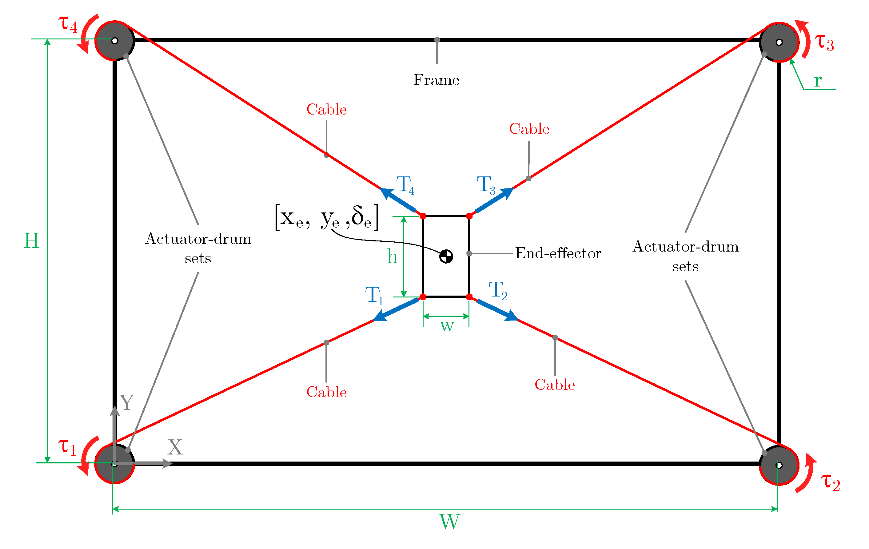
• H and W are the height and width of the frame, respectively.
• h and w are the height and width of the end-effector, respectively.
• $T_i$ for $i=1,\cdots ,4$ the tension of the cables.
• ${\tau }_i$ for $i=1,\cdots ,4$ the torques exerted by each motor.
• r the effective radius of the drums.
• $[x_e,y_e,{\delta }_e]$ the coordinates of the end-effector.

Assuming that no sagging cables are allowed (e.g., [28], the static workspace of the robot can be determined by imposing end-effector poses within the frame and checking if the force/torque equilibrium can be achieved for these poses. The main parameters affecting the workspace are the dimensional parameters of the robot (W, H, w, h, and r), the end-effector mass matrix, $\mathbf{M}$, and the allowable tension limit values: $T_{min}$ and $T_{max}$ [5]. The minimum tension value, $T_{min}$, must be set to avoid sagging cables and low stiffness values. The maximum tension value, $T_{max}$, is determined by the maximum holding torque of the motors and by the breaking strength of the cables [29].

Figure 3 shows the static workspace of the robot scheme of Figure 2 with the parameters of the prototype presented in the experimental results section: $W=2.224$ m, $H=1.112$ m, $w=0.281$ m, $h=0.287$ mm, $m=2$ kg and no rotation of the end-effector $\delta =0^{\circ }$. Figure 3 illustrates that for a minimum tension value, $T_{min}=10$ N, the static workspace is the 70.73% of the frame area. The static workspace is reduced when the allowed minimum tension increases and for $T_{min}=50$ N only the 41.56% of the frame area is accessible to the end-effector.

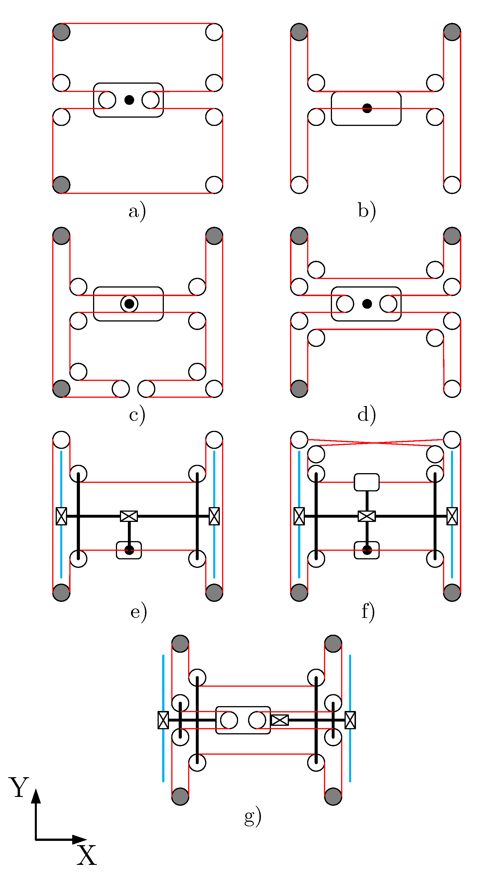
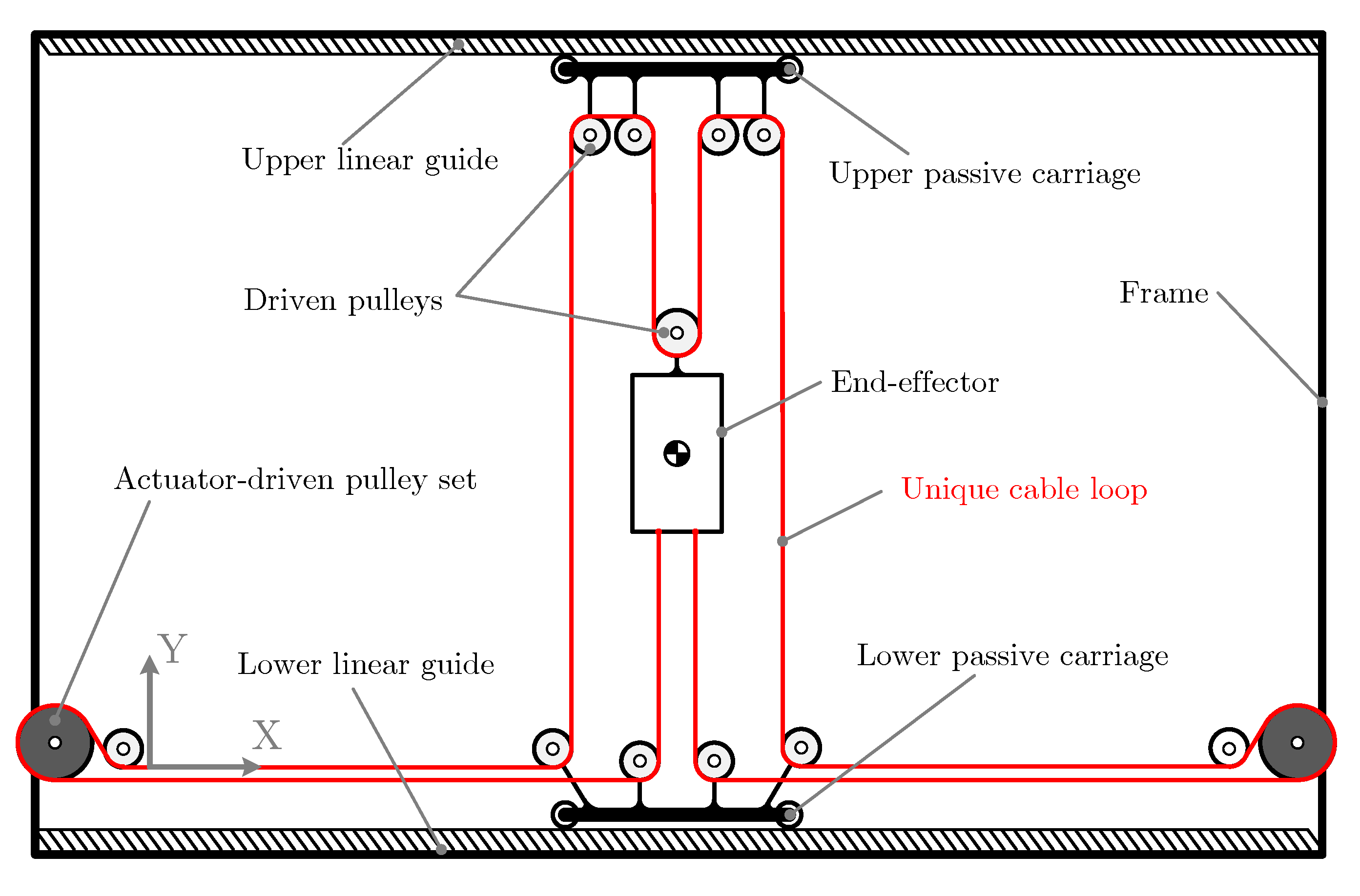
2.2. Novel Single Cable Loop CDPR

As mentioned in Section 1, some of the main drawbacks of CDPR are: (a) the limited workspace inside of the frame [5]; (b) the lack of the robot dexterity when the end-effector is positioned close to the boundaries of the feasible workspace [30].

For solving these two problems, this paper proposes the single cable loop cable-driven parallel robot (sCDPR) scheme shown in Figure 4. The proposal suggests incorporating two sets of passive carriages with linear guides, one in the and one in the lower part of the frame. Through a set of driven pulleys a single cable loop can be designed and its length will remain constant for any pose of the end-effector (assuming negligible in this first step the length variation of the cable due to its elasticity). Two actuators, placed at the lower corners of the frame, provide the movement capability of the end-effector through driven pulleys.

2.3. Nomenclature

Figure 5 shows the sCDPR proposal in an arbitrary pose to present the nomenclature for the modelling of the robot.

The green-coloured dimensional parameters include: W and H, representing the width and height of the frame, w and h, representing the width and height of the end-effector, a representing the distance between the centre of mass of the end-effector and the centre of the driven pulley located at the top of the end-effector, b representing the distance between the centre and the bottom of the end-effector, $w_{uc}$ and $w_{lc}$ representing the widths of the and lower passive carriages, representing the radius of the driver pulleys, and r representing the radius of the driven pulleys attached to the actuators.

The angles of the cables, in red, are α, β and γ which represent the angles with regards to Y axis of the lower inner, inner, and outer paths of the cable loop, respectively.

Being T the pretension of the cable loop, the instant tension of each path of the cable loop has been noted as T, T − ΔT and T + ΔT, and depends on the actuation of the motors attached to the driven pulleys.

The generalised coordinates to develop the model are: q₁, the horizontal coordinate of the end-effector, q₂ the angle with regards to Y axis of the end-effector, q₃ the horizontal coordinate of the lower carriage, and q₄ the horizontal coordinate of the carriage.

Finally, the input torque of both actuators have been noted as τ₁ and τ₂.

2.4. Workspace Gain

With this novel proposal, assuming that after a movement both carriages are almost aligned to the end-effector in the horizontal axis (see the pose of Figure 4 as example), the equilibrium of forces/torque is guaranteed, and the end-effector is therefore able to reach almost all the frame area. In particular, the feasible workspace at static conditions is defined by all end-effector coordinates $[x,y]$ that satisfy:

$$\begin{array}{ccc}\frac{w_{lc}}{2}\hfill & \le x\le & \hfill W-\frac{w_{lc}}{2}\\ b\hfill & \le y\le & \hfill H-a\end{array}$$

(1)

The proposed system, which uses a single closed loop of cable, has a workspace that is solely determined by the geometry of the frame and the end-effector (see expression (1)). Figure 6 illustrates the static workspace of the sCDPR proposal using the same parameters as the results obtained for the conventional scheme. (see Figure 3).

3. Mathematical Model

This section presents the mathematical foundations of the new CDPR design, comprising the kinematic, static, and dynamic models.

3.1. Kinematic Model

In the novel design, the kinematic model is much simpler than that of a conventional CDPR. Owning to the fact that there are only two actuators and one single cable loop, the kinematic model must only take into account the variation of end-effector pose, $\Delta x_e$, $\Delta y_e$, with regards to the angle that the actuators roll up or out the cable, $\Delta {\alpha }_1$, $\Delta {\alpha }_2$. In this sense, the forward kinematic transform yields:

$$[\Delta x_e,\Delta y_e]={\varphi }_{FK}(\Delta {\alpha }_1,\Delta {\alpha }_2),$$

(2)

being ${\varphi }_{FK}=[\frac{r(\Delta {\alpha }_1+\Delta {\alpha }_2)}{2},\frac{r(\Delta {\alpha }_1-\Delta {\alpha }_2)}{2}]$.

The inverse kinematic transform, on the other hand, can be written as:

$$[\Delta {\alpha }_1,\Delta {\alpha }_2]={\varphi }_{IK}(\Delta x_e,\Delta y_e),$$

(3)

being ${\varphi }_{IK}=[\frac{(\Delta x_e-\Delta y_e)}{r},\frac{(\Delta x_e+\Delta y_e)}{r}]$. It is remarkable how both kinematics only depend on the variation of end-effector position, $\Delta x_e,\Delta y_e$, or angular position of the actuators, $\Delta {\alpha }_1,\Delta {\alpha }_2$, and the effective radius of the actuator pulleys, r. The kinematics of the robot are not affected by the tension or pretension of the cables, as shown. However, it does impact the end-effector’s positioning accuracy. This concern is discussed in the Dynamic Model section (Section 3.2), where the effect of pretension on the model is demonstrated.

As the proposal here is based on the use of end-less cables, according to the scheme in Figure 4, the force that the upper cables exert on the end-effector is the same as that exerted by the lower cables, and, therefore, the vertical equilibrium can be statically ensured.

Finally, it is important to mention that a notable advantage of the novel proposal is its kinetostatic simplicity (see (2) and (3)).

3.2. Dynamic Model

The dynamic model has been developed under the assumption that angles $\alpha$, $\beta$ and $\gamma$ (see Figure 5) are small enough to obtain a linear equivalent model. In this way, angles of cables can be originally written as (see Appendix A):

$$\begin{array}{ccc}\alpha & =& {tan}^{-1}\left(\frac{q_3-q_1-asin\left(q_2\right)}{y-acos\left(q_2\right)}\right)\hfill \\ \beta & =& {tan}^{-1}\left(\frac{q_1-q_4-bsin\left(q_2\right)}{H-y-bcos\left(q_2\right)}\right)\hfill \\ \gamma & =& {tan}^{-1}\left(\frac{q_3-q_4}{H}\right)\hfill \end{array}$$

(4)

According to Figure 4, the cable angles are the same on both the left and right sides of the end-effector. In this way, the small angle assumption assumes that the end-effector rotation remains small throughout all manoeuvres, and therefore, the angles of both cables are quasi-similar. Of course, it depends on the cable pretension T and on the end-effector/carriages dimensions.

The dynamics equations of the actuators and carriages have been obtained by writing their Newtonian balances due to their simplicity. For the pose detailed in Figure 5 the torque equilibrium of the motors yields:

$$\begin{array}{c}{\tau }_1+r(T-\Delta T)-rT=0\\ {\tau }_2-r(T+\Delta T)+rT=0\end{array}$$

(5)

Thus, the instantaneous increase in cable loop tension can be expressed as:

$$\Delta T=\frac{{\tau }_1+{\tau }_2}{2R}$$

(6)

The assumption that $\Delta T$ remains constant along the entire single cable route is a strong simplification, and the effective tension actually depends on the length of the cable segment [25]. However, as this model is developed for control purposes, the differences in the dynamics resulting from this assumption can be accounted for by the future dynamic control law for end-effector positioning.

The horizontal equilibrium of the lower carriage force is:

$$-m_3\ddot{q_3}+\frac{1}{R}({\tau }_1+{\tau }_2)-2T\left[sin\left(\gamma \right)+sin\left(\alpha \right)\right]-2T\mu \left[cos\left(\gamma \right)\frac{\dot{q_3}}{|\dot{q_3}|}+cos\left(\alpha \right)\frac{\dot{q_3}}{|\dot{q_3}|}\right]=0$$

(7)

and the horizontal equilibrium of the carriage is:

$$-m_4\ddot{q_4}+2T\left[sin\left(\gamma \right)+sin\left(\beta \right)\right]-2T\mu \left[cos\left(\gamma \right)\frac{\dot{q_4}}{|\dot{q_4}|}+cos\left(\beta \right)\frac{\dot{q_4}}{|\dot{q_4}|}\right]=0$$

(8)

In Equations (7) and (8) $\mu$ is the coefficient of friction of the carriages. The viscous friction has not been considered because of the use of ball-bearing guide carriages.

For obtaining the dynamic behaviour of the end-effector Lagrange formulation has been applied, being the Lagrangian, L:

$$L=\frac{1}{2}{m}_e{\left({\dot{q}}_1\right)}^2+\frac{1}{2}{I}_e{\left({\dot{q}}_2\right)}^2$$

(9)

the equations that describe the dynamics of the end-effector are:

$$\begin{array}{ccc}\hfill \frac{d}{dt}\left(\frac{\partial L}{\partial {\dot{q}}_1}\right)+\frac{\partial L}{\partial q_1}& =& Q_1\hfill \\ \hfill \frac{d}{dt}\left(\frac{\partial L}{\partial {\dot{q}}_2}\right)+\frac{\partial L}{\partial q_2}& =& Q_2\hfill \end{array}$$

(10)

where $Q_1$ is the generalised horizontal force and $Q_2$ the generalised torque. Assuming that:

$$d{W}_t=Q_{1}d{q}_1+Q_{2}d{q}_2$$

(11)

being $W_t$ the total work exerted by $Q_1$ and $Q_2$. If $d{W}_t$ is determined $Q_1$ and $Q_2$ can be therefore obtained. Assuming the end-effector scheme of Figure 7 $d{W}_t$ can be determined with by computing the work exerted at points A and B as:

$$d{W}_t=d{W}_A+d{W}_B$$

(12)

being $d{W}_A={\mathbf{F}}_{A}d{\mathbf{r}}_A$ and $d{W}_B={\mathbf{F}}_{B}d{\mathbf{r}}_B$. The A and B differential position arrays can be written as:

$$\begin{array}{cccc}d{\mathbf{r}}_A& =& [d{q}_1+acos\left(q_2\right)d{q}_2,\hfill & \hfill asin\left(q_2\right)d{q}_2]\\ d{\mathbf{r}}_B& =& [d{q}_1+bcos\left(q_2\right)d{q}_2,\hfill & \hfill -bsin\left(q_2\right)d{q}_2]\end{array}$$

(13)

and the Forces applied at A and B points as:

$$\begin{array}{ccccc}{\mathbf{F}}_A& =\hfill & [& \hfill 2Tsin\left(\alpha \right),& \hfill -2Tcos\left(\alpha \right)]\\ {\mathbf{F}}_B& =\hfill & [& \hfill -2Tsin\left(\beta \right),& \hfill 2Tcos\left(\beta \right)]\end{array}$$

(14)

The differential of the total work can be easily obtaining by substituting (13) and (14) in (12):

$$\begin{array}{ccc}\hfill d{W}_t& =& 2T[sin\left(\alpha \right)+d{q}_1+asin\left(\alpha \right)cos\left(q_2\right)d{q}_2-acos\left(\alpha \right)sin\left(q_2\right)d{q}_2]+\hfill \\ \hfill & & 2T[-sin\left(\beta \right)d{q}_1+bsin\left(\beta \right)cos\left(q_2\right)d{q}_2-bcos\left(\beta \right)sin\left(q_2\right)d{q}_2]\hfill \end{array}$$

(15)

Identifying (11) with (15), $Q_1$ and $Q_2$ can be finally determined:

$$\begin{array}{c}{Q}_1=2T(sin\left(\alpha \right)-sin\left(\beta \right))\\ Q_2=2T(asin(\alpha -q_2)+bsin(\beta -q_2))\end{array}$$

(16)

By assuming small values of $q_2$ and that the horizontal distance between both carriages is much smaller than the vertical distance, i.e., $|q_3-q_1|<<Y$, $|q_4-q_1|<<H-Y$ and $|q_3-q_4|<<H$, angles in (4) can be assumed to be:

$$\begin{array}{ccc}\alpha & \approx & \frac{q_3-q_1-asin\left(q_2\right)}{y-acos\left(q_2\right)}\\ \beta & \approx & \frac{q_1-q_4-bsin\left(q_2\right)}{H-y-bcos\left(q_2\right)}\\ \gamma & \approx & \frac{q_3-q_4}{H}\end{array}$$

(17)

In this way, developing expressions (10) a linear and time invariant (LTI) dynamic model is finally achieved and expressed as:

$$\mathbf{M}\ddot{\mathbf{q}}\left(t\right)+\mathbf{K}\mathbf{q}\left(t\right)=\mathbf{w}$$

(18)

being $\mathbf{M}$, the mass/inertia matrix:

$$\mathbf{M}=\left(\begin{array}{cccc}{m}_e& 0& 0& 0\\ 0& I_e& 0& 0\\ 0& 0& m_3& 0\\ 0& 0& 0& m_4\end{array}\right)$$

(19)

$\mathbf{K}$ the stiffness matrix:

$$\mathbf{K}=\left(\begin{array}{cccc}2T\left(\frac{1}{z_2}+\frac{1}{z_1}\right)& 2T\left(\frac{a}{z_2}-\frac{b}{z_1}\right)& -\frac{2T}{z_2}& -\frac{2T}{z_1}\\ 2T\left(\frac{1}{z_2}-\frac{1}{z_1}\right)& 2T\left(\frac{a^2}{z_2}+a+\frac{b^2}{z_1}+b\right)& -\frac{2Ta}{z_2}& \frac{2Tb}{z_1}\\ -\frac{2T}{z_2}& -\frac{2Ta}{z_2}& 2T\left(\frac{1}{H}+\frac{1}{z_2}\right)& -\frac{2T}{H}\\ -\frac{2T}{z_1}& \frac{2Tb}{z_1}& -\frac{2T}{H}& 2T\left(\frac{1}{H}+\frac{1}{z_1}\right)\end{array}\right)$$

(20)

with $z_1=H-Y-b$, $z_2=Y-a$ and $\mathbf{w}$ the external force array:

$$\mathbf{w}=\left(\begin{array}{c}0\\ 0\\ \frac{1}{R}({\tau }_1+{\tau }_2)-4T\mu \frac{\dot{q_3}}{|\dot{q_e}|}\\ -4T\mu \frac{\dot{q_4}}{|\dot{q_4}|}\end{array}\right)$$

(21)

The dynamic model (18) is valid as long as the small cable angle assumption is fulfilled. The accuracy of the proposed LTI model in describing the dynamics of the sCDPR will be demonstrated through simulation and experimental results. In addition, model (18) is intentionally simplified by not considering external forces such as gravity. That is because the influence of gravity on the dynamic model is minimal. This is due to the design of the proposal, which utilises a significantly larger pretension value compared with the force exerted by gravity on the end-effector. Furthermore, the pretension applies four times to the end-effector, with two upper cables and two lower cables.

From a control scheme perspective, the linearity of model (18) implies that the influence of gravity action merely alters the system’s equilibrium point without affecting the control law.

4. Experimental Platform Description

4.1. Robot Description

The experimental platform has been designed to be mainly built by laser cutting and 3D printed parts. Figure 8 shows the design and the final prototype, including the main functional elements.

The frame and end-effector are made of 4 mm steel plates cut by laser. The pulleys have been printed with micro carbon fibre filled nylon and the cable is a 2 mm of diameter steel cable. The actuators are two DC motors, MaxonMotor RE40, with a 26:1 gearbox. They also included 256 ppr (pulses per revolution) encoders to acquire their angular position. The motors are commanded by two servoamplifiers, ESCON 70/10 which receive the control signal from the control device: a NI MyRio 1900 real-time controller. This configuration ensures a sampling frequency of 1 KHz.

Table 1. Parameters of the prototype.

Frame
Width, W (mm)	2224
Height, H (mm)	1112
End-effector
Width, w (mm)	287
Height, h (mm)	281
Mass, $m_e$ (kg)	2.1
Rotational Inertia, $I_e$ (kg · m ${}^2$)	2.5198 · ${10}^{-2}$
Cable
Diameter, d (mm)	2
Young’s module, E (GPa)	2.0912
Passive Carriages
Width, $w_3=w_4$ (mm)	287
Mass, $m_3=m_4$ (kg)	1.2
Motor/Pulley sets
Rotational Inertia, J (kg · m ${}^2$)	$1.2734·{10}^{-2}$
Viscous friction coefficient, b (Nms)	0.2
Effective radius, r (mm)	7.3

summarises the main parameters of the robot, where J and b are, respectively, the rotational inertia and the viscous friction coefficient of the motor/gearbox/driver pulley sets.

4.2. Computer Vision System

In front of the robot, a vision system is placed to track some points of interest during the robot’s manoeuvres. Four markers have been attached to the frame, four to the end-effector, and one at each passive carriage.

The camera has 8 Megapixels with a 3264 × 2448 resolution and a Sony IMX179 sensor. The focal distance and brightness can be manually adjusted. After the camera calibration, the 30 fps images are undistorted, and the equivalence between image coordinates and world coordinates is obtained. The different points of interest are obtained by simple colour segmentation, and the position of the end-effector and passive carriages can therefore be obtained after the experiments in an offline way. Owing to the camera resolution (3264 × 2448 px) and the robot size (2224 × 1112 mm), after removing the unused image region and after the camera calibration procedure, the maximum estimated reprojection error is about 0.26 px which corresponds in world coordinates to 0.19 mm. This is the expected maximum error committed by the vision system for the position estimations [31].

Figure 9 represents, as an example, a region of interest of the original image, the marker pose detection by segmentation and the end-effector position estimation (Supplementary Video).

5. Model Identification and Validation

5.1. Parameters Identification

The objective of this section is to validate the dynamic model developed in Section 3.2. Dimensional parameters (see Table 1) can be directly measured, but the coefficient of friction, $\mu$, shall be identified.

For this purpose, some experiments have been carried out. For a given cable loop pretension value ($T=350$ N), the voltages that control the servoamplifiers have been increased in 0.1 V steps in both motors, observing the first voltage value when carriages (and end-effector) start moving. By repeating the experiment 30 times, the average value of voltage is $V_f=0.68$ V, which corresponds to a motor torque of ${\tau }_f=0.3284$ Nm.

These experiments are open-loop experiments and both motor are excited with the same voltage signals, $V_1=V_2=V$. The equivalence between the reference voltage signal and the current reference signal, $I_1^{*}=I_2^{*}=I^{*}$, can be configured in the servoamplifier to use all the DAQ resolution. In this sense, a $V^{*}=\pm 10$ V reference voltage signal corresponds to a $I^{*}=\pm 6$ A reference current signal (nominal current of the DC motors). Therefore, the servoamplifier closes the current control loop taking as reference this current reference signal. The exerted torque of the motor is assumed to be $\tau =K_e{I}^{*}$, being $K_e$ the torque constant of the motor provided by the motor supplier (Maxon Motor) $K_e=30.2$ mNm/A.

On the other hand, the dynamic model (18) has been implemented in Matlab^®/Simulink^® and both motors have been excited with ${\tau }_f=0.3268$ Nm. Changing the value of $\mu$, the one that minimises the error between the experimental and simulated results has been selected, $\mu =0.1723$.

For illustrative purposes, Figure 10 compares the first 10 experimental results and the simulated one after identifying $\mu$ value. The horizontal position of the carriage, $q_4$, initially placed at $q_4\left(0\right)=0.2$ m, is represented when $V_f$ is applied in both motors.

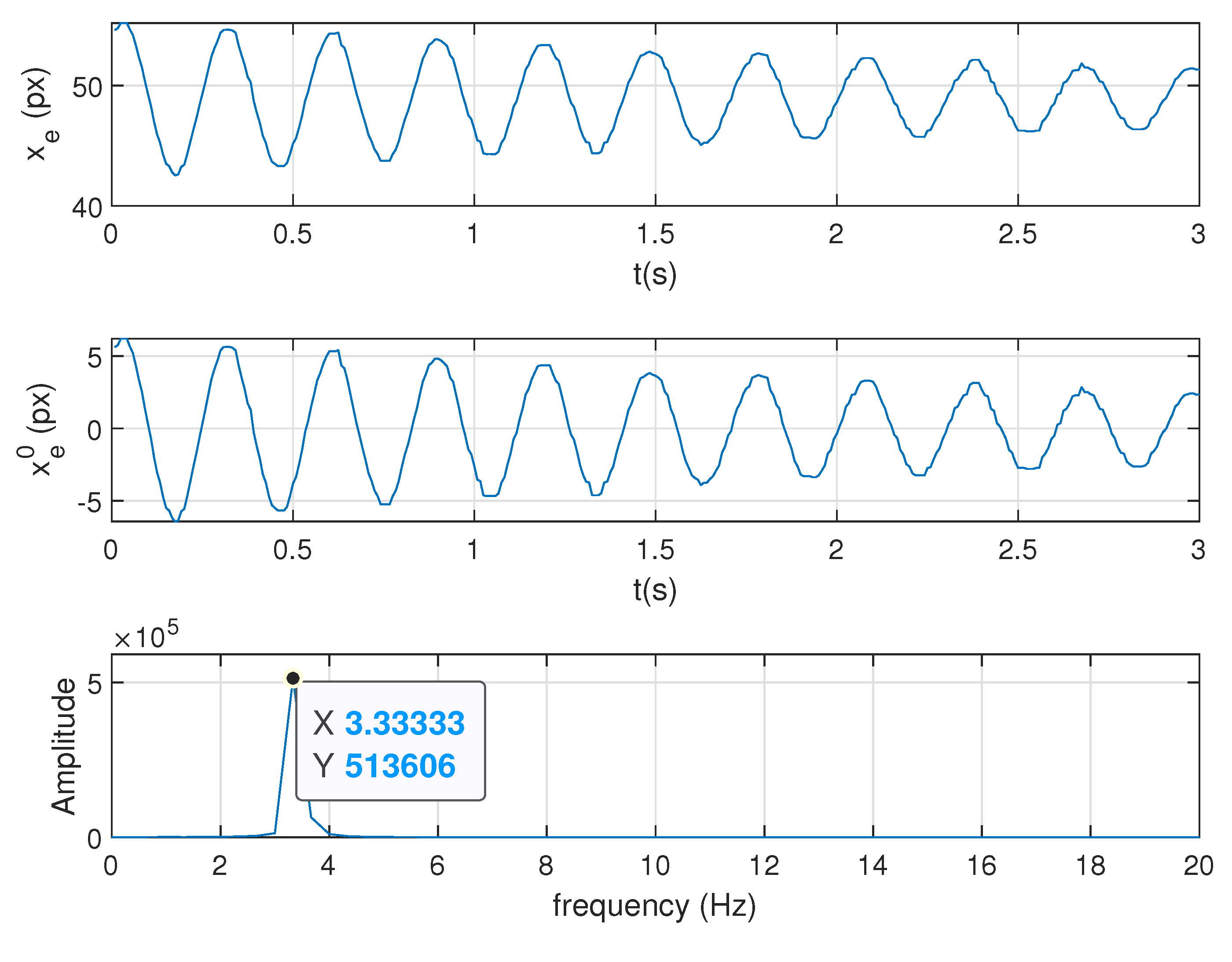
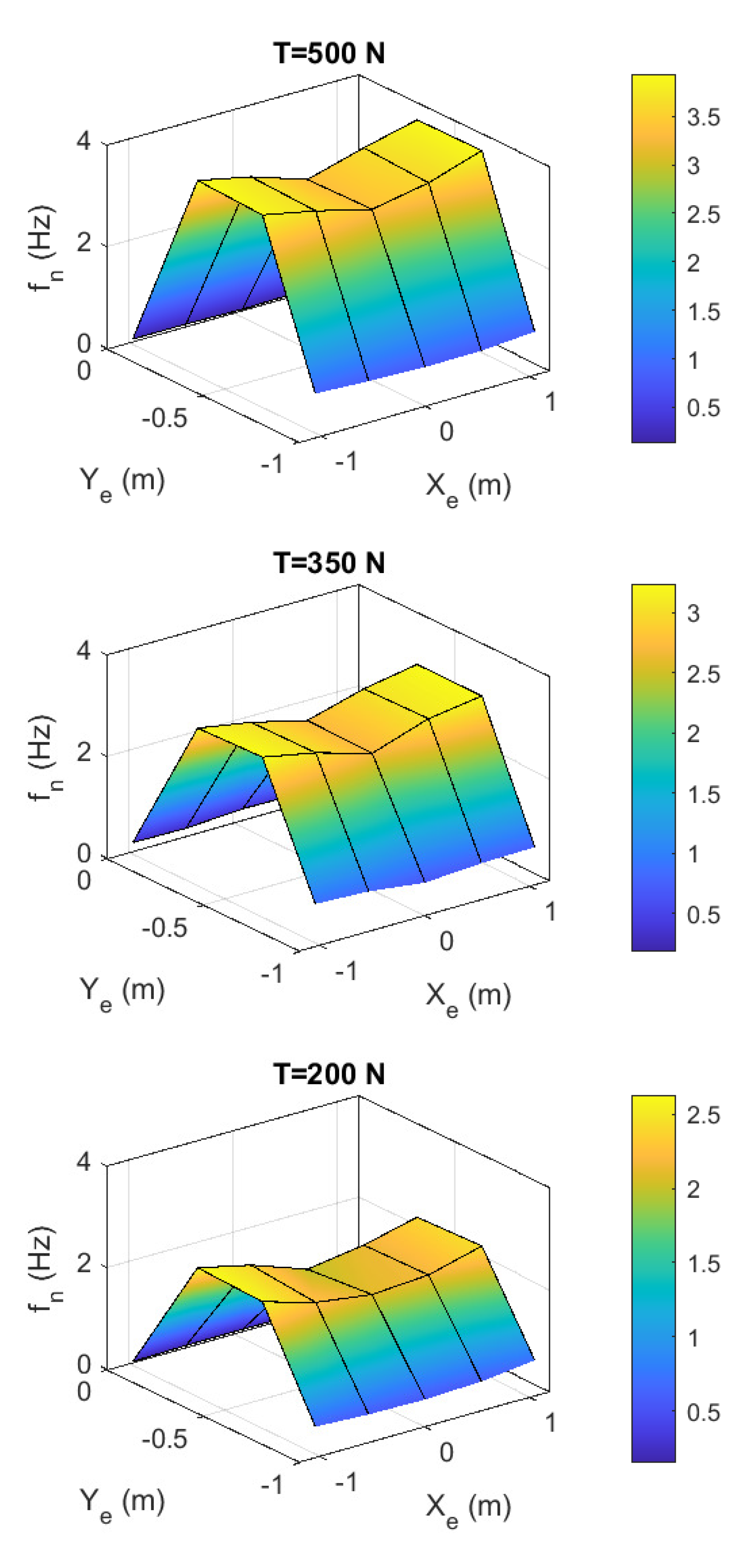
5.2. Frequency Characterisation

This section aims to determine the natural frequency of the robot, which will be utilised in upcoming control strategies to counteract any end-effector vibration during robot manoeuvres. The cable loop pretension value, T, has a notorious influence on this natural frequency. In this way, this frequency has been determined for three values of cable pretension: a low value of 200 N, a medium value of 350 N, and a high value of 500 N.

The procedure to obtain the natural frequency is based on the pseudoimpulse response of the system. For a given end-effector position, an horizontal external force is applied to it; the vision system described in Section 4.2 registers the end-effector pose; its horizontal displacement is therefore acquired, $x_e$; its mean value, $x_e^0$, is removed; and FFT is applied to determine the maximum frequency peak of the frequency spectrum by peak picking. Note that a clear single peak appears in the frequency spectrum. Figure 11 illustrates this procedure.

By repeating the aforementioned procedure for different positions (4 positions on the vertical axis and 5 positions on the horizontal axis), Figure 12 illustrates the natural frequency of the end-effector, denoted as $f_n$ in Hz.

Note that natural frequency is low when the end-effector is placed near the top or bottom of the frame, and it grows up when the vertical position is near the centre of the frame, where it reaches its maximum value. For higher values of cable loop pretension, the natural frequency is about 3.9 Hz, and for lower values of pretension, it is about 2.4 Hz.

The frequency characterization obtained can be utilised in designing a control strategy aimed at mitigating any undesired vibration of the end-effector during its manoeuvres.

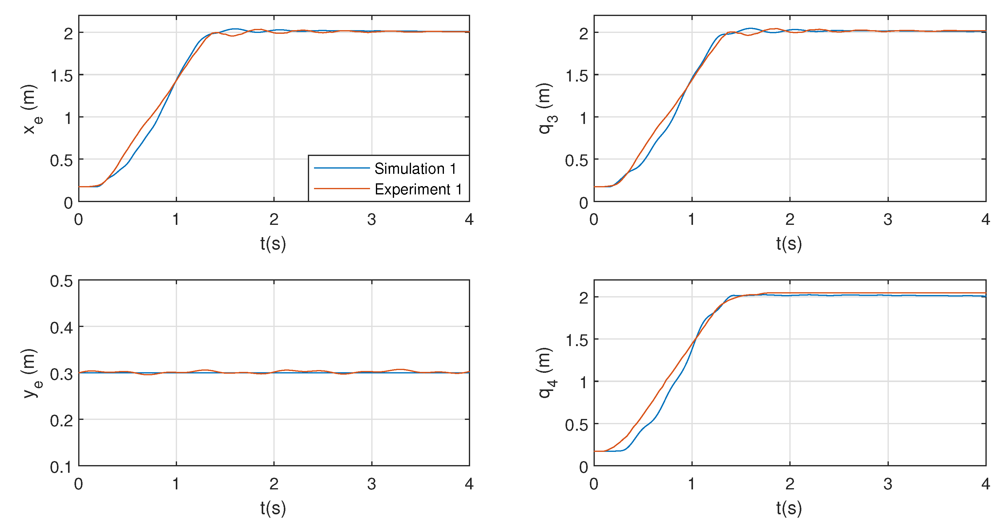
5.3. Model Validation

Simulated and experimental results are compared in this section for validation purposes. The experiments consist of placing the end-effector in an initial pose and applying a 1-second torque step to both motors. The experiments carried out are summarised in

Table 2. Summary of open-loop experiments for validation.

Experiment	End-Effector Position	Input Torques
	$[{\mathit{x}}_{\mathit{e}},{\mathit{y}}_{\mathit{e}}]$ m	$[{\mathit{\tau }}_1,{\mathit{\tau }}_2]$ Nm
1	$[0.173,0.300]$	$[4.85,4.85]$
2	$[1.830,0.300]$	$[-4.78,-4.78]$
3	$[0.550,0.234]$	$[1.87,-1.87]$
4	$[0.550,0.921]$	$[-1.82,1.82]$

. These experiments are executed in open-loop, and the values of the torques have therefore been selected to avoid the collision of the end-effector/carriages with the frame while providing large movements of the end-effector.

For all experiments, the end-effector position and the carriage positions are compared.

For illustrative purposes, Figure 13 shows the simulated and experimental results of Experiment 1 in Table 2. The input torques of the four experiments are represented in Figure 14.

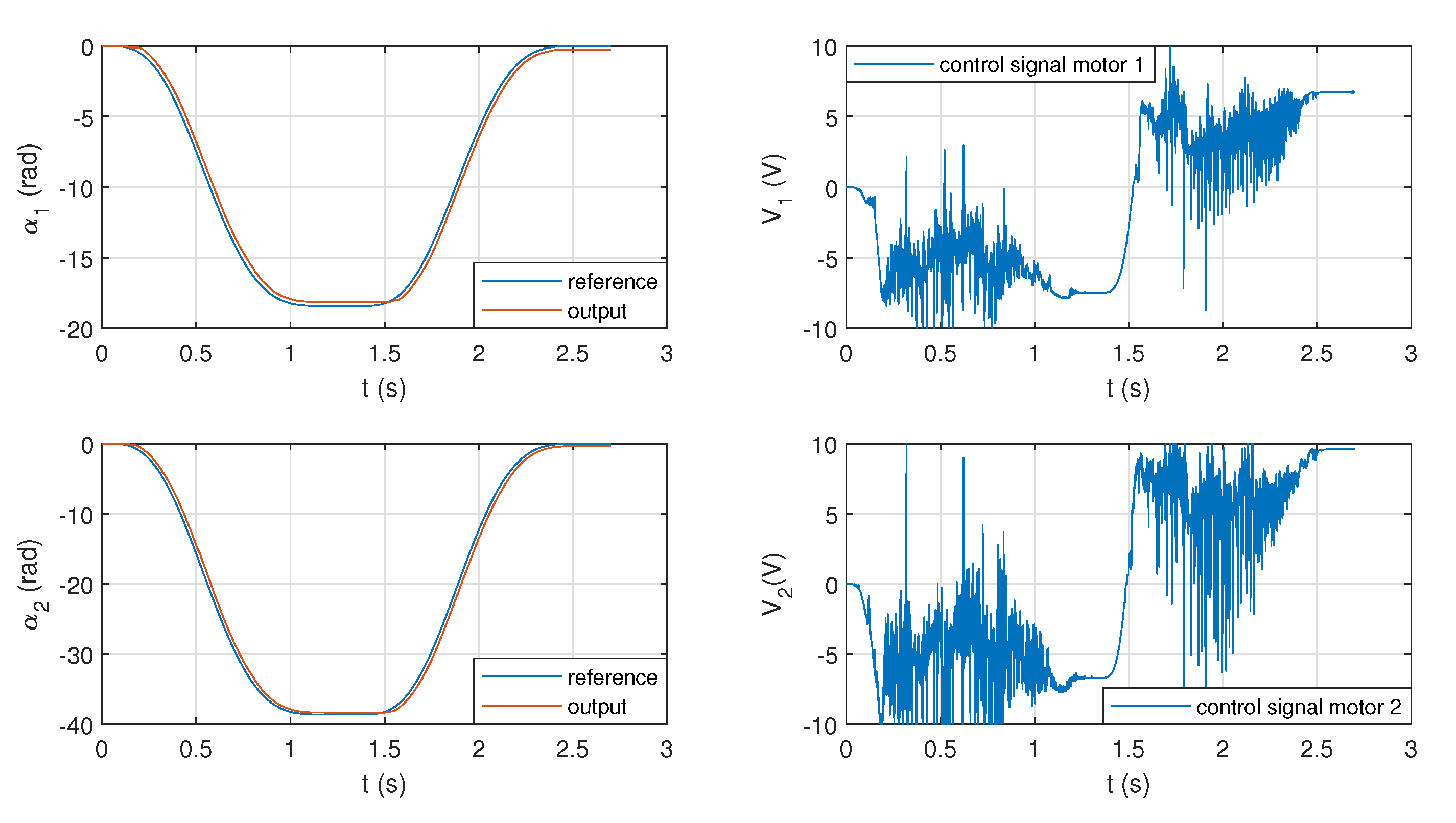
6. Kinematic Control

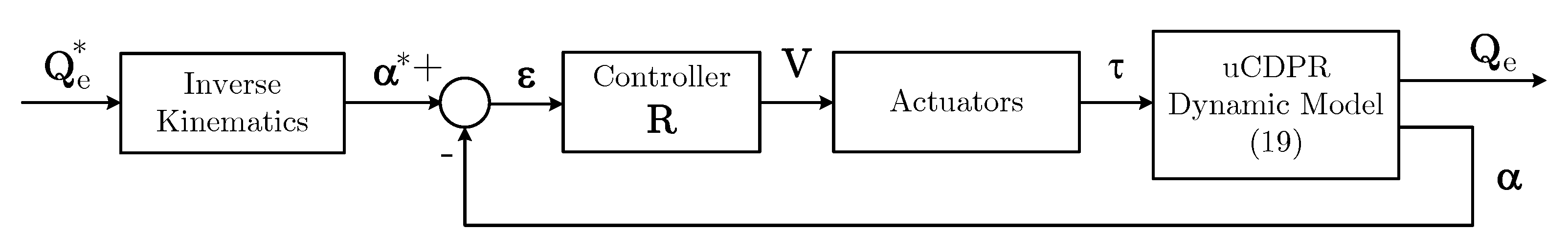
This section is devoted to showing the controllability of the system by means of a simple kinematic control.

6.1. Control Scheme

To illustrate the workspace gain of the proposal and the controllability of the system, the kinematic control shown in Figure 15 is experimentally implemented. This control scheme assumes that the dynamics of the actuators are decoupled from the sCDPR, i.e., kinematic control is applied as a first approach (e.g., [32]).

In Figure 15 ${\mathbf{Q}}_e^{*}={[x_e^{*},y_e^{*}]}^T$ is the end-effector position reference, ${\alpha }^{*}={[{\alpha }_1^{*},{\alpha }_2^{*}]}^T$ is the joint coordinates reference, $\epsilon ={[{\alpha }_1^{*}-{\alpha }_1,{\alpha }_2^{*}-{\alpha }_2]}^T$ the error signal, $\mathbf{V}={[V_1,V_2]}^T$ are the voltage control signal, $\tau ={[{\tau }_1,{\tau }_2]}^T$ the input torque, ${\mathbf{Q}}_e={[x_e,y_e]}^T$ the end-effector pose and $\alpha ={[{\alpha }_1,{\alpha }_2]}^T$ the actual joint coordinates.

In this way, as control scheme is based in joint coordinates space, controller block, $\mathbf{R}$ in Figure 15 is:

$$\mathbf{R}=\left[\begin{array}{cc}{R}_1& 0\\ 0& R_2\end{array}\right]$$

(22)

where $R_1=R_2=R$ due to mechanical symmetry in the robot design.

To illustrate the controllability of the system a linear PD controller is designed for each actuator set. Its control law can be written as:

$$V_i\left(t\right)=K_p{\epsilon }_i\left(t\right)+K_d\frac{d{\epsilon }_i\left(t\right)}{dt}$$

(23)

for actuator $i=1,2$.

The prototype is actuated by means of two DC motor/gearbox/driver pulley sets, which allow the following transfer functions to be identified for the motors:

$$G\left(s\right)=\frac{\alpha \left(s\right)}{V\left(s\right)}=\frac{1/J}{s(s+b/J)}=\frac{2169}{s(s+16.68)}$$

(24)

The identification of the transfer function of the DC motor has follow the well-known procedure based on its speed step response. More details can be seen at [33].

Given the frequency requirements of a gain crossover frequency of ${\omega }_c=40$ rad/s and a phase margin of ${\phi }_m={60}^{\circ }$ (see [34,35]), the resulting controller is:

$$R\left(s\right)=0.6352+0.0125s$$

(25)

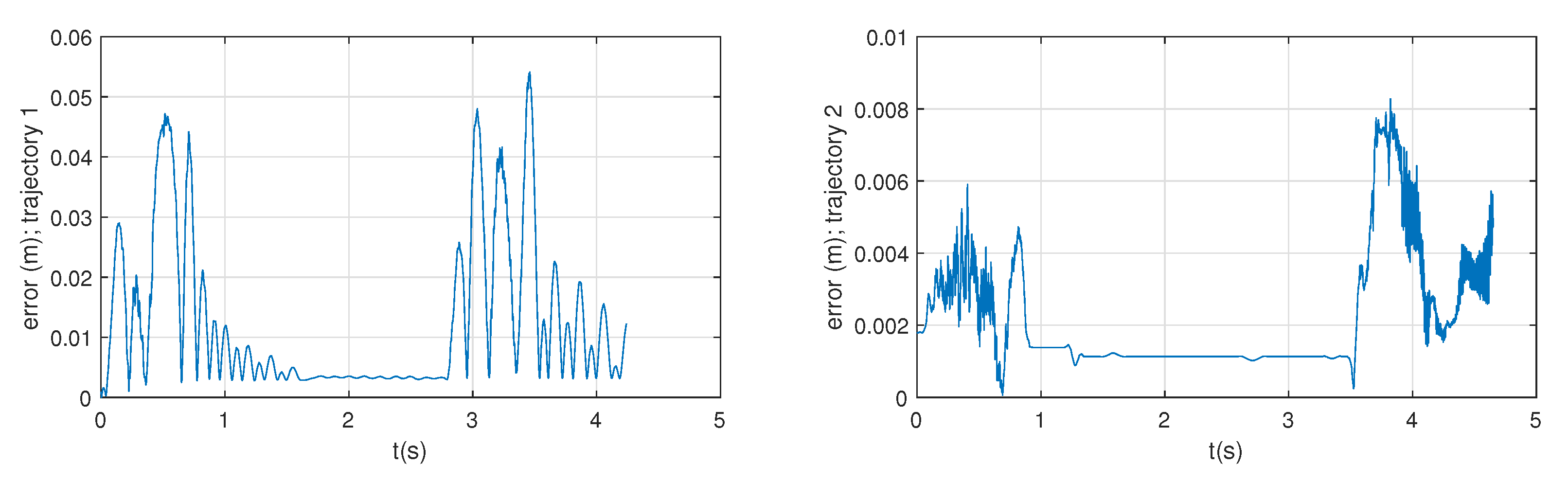
6.2. Position Control Results

Two simple manoeuvres have been experimentally tested: one horizontal and one vertical. Since the actuators model (24) is of second order, 4th order Bezier trajectories were implemented to ensure smooth end-effector trajectories. Both trajectories start at the initial pose of the end-effector, execute a manoeuvre to an intermediate pose, and return to the initial pose.

Table 3. Kinematic control trajectories.

Trajectory	Initial Pose	Intermediate Pose	Final Pose	Trajectory Time
	$[{\mathbf{x}}_{\mathbf{e}},{\mathbf{y}}_{\mathbf{e}}]$m			${\mathbf{t}}_{\mathbf{s}}$(s)
Horizontal	$[0.3,0.55]$	$[1.9,0.55]$	$[0.3,0.55]$	4
Vertical	$[0.55,0.20]$	$[0.55,0.9]$	$[0.55,0.20]$	4.5
Diagonal	$[2.08,0.92]$	$[0.01,0.19]$	$[2.08,0.92]$	2.5

summarises the initial and final end-effector poses and the trajectory times of both controlled manoeuvres.

Figure 16 and Figure 17 represent the reference tracking of the horizontal and vertical trajectories of Table 3. Note that the end-effector suffers some vibration during the manoeuvres in coherence with Section 5.2. The objective of this paper is to present the advantages of the novel sCDPR scheme and its dynamic model. The control approach presented here will be treated in further works in order to improve the accuracy of the robot by compensating for the undesirable vibration during its movement.

Figure 18 represents the Euclidean error, ${\epsilon }_e$, committed during the trajectories:

$${\epsilon }_e\left(t\right)=\sqrt{{(x_e^{*}\left(t\right)-x_e\left(t\right))}^2+{(y_e^{*}\left(t\right)-y_e\left(t\right))}^2}$$

(26)

Note that, although a simple kinematic control has been implemented, for horizontal manoeuvres the maximum error appears during the acceleration and deceleration phases, at about 50 mm, and for vertical manoeuvres about 8 mm.

Finally, Figure 19 represents the trajectory tracking of a diagonal movement. This trajectory is faster than the previous ones. Figure 20 shows the joint control and the control signal of both motors. Note that in this last case, the control signal is near the saturation limit of $[-10,10]$ V.

For the trajectory tracking experiments in Table 3, the end-effector angle has been measured with the vision system. The maximum absolute value of the end-effector angle was $|{\delta }_e|=3.2^{\circ }$ (see Figure 19).

7. Conclusions

In this paper, a novel design for planar fully-constrained CDPRs of 2 DOFs is proposed. The design is a mechanical modification of the one presented in ref. [19], where a single cable loop is used instead of four different cables.

The innovative CDPR consists of two passive carriages that move freely along linear guides attached to the robot frame and a single cable loop driven by two actuators. The end-effector’s pose is altered by a set of driven pulleys while keeping the cable length constant.

The primary objective of the new design is to expand the robot’s feasible workspace compared with conventional designs. In addition, the stiffness of the robot remains invariant for a given pretension of the cable loop.

After presenting the novel sCDPR scheme, the kinetostatic problem is introduced. One of the advantages of this new design is the simplicity of both forward and inverse kinematic transforms. The single cable loop reduces the kinematics to expressions where the variation of pose of the end-effector is directly related to the variation of cable roll in or out by the motors, which are much simpler than the kinematic formulations of the previous CDPR models in [19].

The dynamic model of the system has also been developed, bringing a linear and time-invariant model that allows for direct application of linear techniques. The dynamic model has been developed under the assumption that end-effector and passive carriages are pseudo-aligned and cable angles are small. Experimental results have been carried out to validate the dynamic model developed.

Finally, a simple kinematic control has been experimentally applied to illustrate the controllability of the system. The kinematic control has been designed considering only the dynamics of the actuators. Experimental results show an acceptable error for end-effector trajectory tracking.

For removing the residual vibration of the end-effector during horizontal manoeuvres further work will propose more complex control strategy approaches based on the frequency characterisation of the sCDPR.

The work presented here will continue with the design and implementation of a dynamic control to obtain accurate end-effector trajectory tracking. A dynamic control strategy based on the frequency characterisation shown in Section 5.2 and dynamics inversion will be applied as a first step. Owing to the natural creep of steel cables, a tension sensor [36] and an a active linear actuator will be added to the system for maintenance purposes (see Figure 21).

In addition, more complex control strategies will employ the linear actuator to control the end-effector pose during the robot manoeuvres. The presented scheme can be applied to any planar application where CDPR can be applied. In particular, the complete controller system, including the active tensor and the tension sensor, will be applied to a system for automated cleaning of a solar panel array, for an automated storage and retrieval system, and for inspecting the lower size of bridges decks.

References

1. Gouttefarde, M.; Bruckmann, T. Cable-Driven Parallel Robots. In Encyclopedia of Robotics; Springer: Berlin/Heidelberg, Germany, 2022; pp. 1–14. [Google Scholar]
2. Verhoeven, R. Analysis of the Workspace of Tendon Based Stewart Platforms. Ph.D. Thesis, University of Duisburg, Essen, Germany, 2006. [Google Scholar]
3. Tho, T.P.; Thinh, N.T. An Overview of Cable-Driven Parallel Robots: Workspace, Tension Distribution, and Cable Sagging. Math. Probl. Eng. 2022, 2022, 2199748. [Google Scholar] [CrossRef]
4. Zi, B.; Duan, B.; Du, J.; Bao, H. Dynamic modeling and active control of a cable-suspended parallel robot. Mechatronics 2008, 18, 1–12. [Google Scholar] [CrossRef]
5. Pott, A. Cable-Driven Parallel Robots; Springer Science & Business Media: Berlin/Heidelberg, Germany, 2018; Volume 1. [Google Scholar]
6. Qian, S.; Zi, B.; Shang, W.W.; Xu, Q.S. A review on cable-driven parallel robots. Chin. J. Mech. Eng. 2018, 31, 66. [Google Scholar] [CrossRef]
7. Ming, A. Study on multiple degree-of-freedom positioning mechanism using wires (part 1). Int. J. Jpn. Soc. Precis. Eng. 1994, 28, 131–138. [Google Scholar]
8. Lv, W.; Tao, L.; Ji, Z. Sliding mode control of cable-driven redundancy parallel robot with 6 DOF based on cable-length sensor feedback. Math. Probl. Eng. 2017, 2017, 1928673. [Google Scholar] [CrossRef]
9. Pott, A. On the limitations on the lower and upper tensions for cable-driven parallel robots. In Advances in Robot Kinematics; Springer: Berlin/Heidelberg, Germany, 2014; pp. 243–251. [Google Scholar]
10. Gagliardini, L.; Caro, S.; Gouttefarde, M.; Girin, A. Discrete reconfiguration planning for cable-driven parallel robots. Mech. Mach. Theory 2016, 100, 313–337. [Google Scholar] [CrossRef]
11. Youssef, K.; Otis, M.J.D. Reconfigurable fully constrained cable driven parallel mechanism for avoiding interference between cables. Mech. Mach. Theory 2020, 148, 103781. [Google Scholar] [CrossRef]
12. An, H.; Yuan, H.; Tang, K.; Xu, W.; Wang, X. A Novel Cable-Driven Parallel Robot With Movable Anchor Points Capable for Obstacle Environments. IEEE/ASME Trans. Mechatron. 2022, 27, 5472–5483. [Google Scholar] [CrossRef]
13. Tan, H.; Nurahmi, L.; Pramujati, B.; Caro, S. On the reconfiguration of cable-driven parallel robots with multiple mobile cranes. In Proceedings of the 2020 5th International Conference on Robotics and Automation Engineering (ICRAE), Singapore, 20–22 November 2020; pp. 126–130. [Google Scholar]
14. Barbazza, L.; Oscari, F.; Minto, S.; Rosati, G. Trajectory planning of a suspended cable driven parallel robot with reconfigurable end effector. Robot.-Comput.-Integr. Manuf. 2017, 48, 1–11. [Google Scholar] [CrossRef]
15. Rodriguez-Barroso, A.; Saltaren, R.; Portilla, G.A.; Cely, J.S.; Carpio, M. Cable-driven parallel robot with reconfigurable end effector controlled with a compliant actuator. Sensors 2018, 18, 2765. [Google Scholar] [CrossRef] [PubMed]
16. Wang, R.; Li, Y. Analysis and multi-objective optimal design of a planar differentially driven cable parallel robot. Robotica 2021, 39, 2193–2209. [Google Scholar] [CrossRef]
17. Duan, Q.; Vashista, V.; Agrawal, S.K. Effect on wrench-feasible workspace of cable-driven parallel robots by adding springs. Mech. Mach. Theory 2015, 86, 201–210. [Google Scholar] [CrossRef]
18. Castillo-Garcia, F.J.; Rubio-Gómez, G.; Juárez, S.; Rodríguez-Rosa, D.; Bravo, E.; Ottaviano, E.; Gonzalez-Rodriguez, A. Addition of passive-carriage for increasing workspace of cable robots: Automated inspection of surfaces of civil infrastructures. Smart Struct. Syst. Int. J. 2021, 27, 387–396. [Google Scholar]
19. Martin-Parra, A.; Juarez-Perez, S.; Gonzalez-Rodriguez, A.; Gonzalez-Rodriguez, A.G.; Lopez-Diaz, A.I.; Rubio-Gomez, G. A novel design for fully constrained planar Cable-Driven Parallel Robots to increase their wrench-feasible workspace. Mech. Mach. Theory 2023, 180, 105159. [Google Scholar] [CrossRef]
20. Li, J.; Wang, K.; Wang, Y.; Wang, C. Motion Planning for a Cable-Driven Lower Limb Rehabilitation Robot with Movable Distal Anchor Points. J. Bionic Eng. 2023, 1–12. [Google Scholar] [CrossRef]
21. Behzadipour, S. Kinematics and Dynamics of a Self-Stressed Cartesian Cable-Driven Mechanism. J. Mech. Des. 2009, 131, 061005. [Google Scholar] [CrossRef]
22. Laliberte, T.; Gosselin, C.M.; Gao, D. Closed-loop transmission routings for cartesian scara-type manipulators. In Proceedings of the International Design Engineering Technical Conferences and Computers and Information in Engineering Conference, Montreal, QC, Canada, 15–18 August 2010; Volume 44106, pp. 281–290. [Google Scholar]
23. Gosselin, C.; Laliberté, T.; Mayer-St-Onge, B.; Foucault, S.; Lecours, A.; Duchaine, V.; Paradis, N.; Gao, D.; Menassa, R. A friendly beast of burden: A human-assistive robot for handling large payloads. IEEE Robot. Autom. Mag. 2013, 20, 139–147. [Google Scholar] [CrossRef]
24. Borboni, A.; Ceretti, E.; Copeta, A.; Moscatelli, D.; Faglia, R.; Attanasio, A. High precision machine based on a differential mechanism. In Engineering Systems Design and Analysis; American Society of Mechanical Engineers: New York, NY, USA, 2014; Volume 45844, p. V002T16A001. [Google Scholar]
25. Idà, E.; Nanetti, F.; Mottola, G. An Alternative Parallel Mechanism for Horizontal Positioning of a Nozzle in an FDM 3D Printer. Machines 2022, 10, 542. [Google Scholar] [CrossRef]
26. Barrette, G.; Gosselin, C.M.M. Determination of the dynamic workspace of cable-driven planar parallel mechanisms. J. Mech. Des. 2005, 127, 242–248. [Google Scholar] [CrossRef]
27. Williams Ii, R.L.; Gallina, P. Translational planar cable-direct-driven robots. J. Intell. Robot. Syst. 2003, 37, 69–96. [Google Scholar] [CrossRef]
28. Ottaviano, E.; Arena, A.; Gattulli, V. Geometrically exact three-dimensional modeling of cable-driven parallel manipulators for end-effector positioning. Mech. Mach. Theory 2021, 155, 104102. [Google Scholar] [CrossRef]
29. Yuan, H.; Courteille, E.; Deblaise, D. Static and dynamic stiffness analyses of cable-driven parallel robots with non-negligible cable mass and elasticity. Mech. Mach. Theory 2015, 85, 64–81. [Google Scholar] [CrossRef]
30. Abdolshah, S.; Zanotto, D.; Rosati, G.; Agrawal, S.K. Optimizing stiffness and dexterity of planar adaptive cable-driven parallel robots. J. Mech. Robot. 2017, 9, 031004. [Google Scholar] [CrossRef]
31. Fetić, A.; Jurić, D.; Osmanković, D. The procedure of a camera calibration using Camera Calibration Toolbox for MATLAB. In Proceedings of the 35th International Convention MIPRO, Opatija, Croatia, 21–25 May 2012; pp. 1752–1757. [Google Scholar]
32. Tang, J.; Zhang, Y.; Huang, F.; Li, J.; Chen, Z.; Song, W.; Zhu, S.; Gu, J. Design and kinematic control of the cable-driven hyper-redundant manipulator for potential underwater applications. Appl. Sci. 2019, 9, 1142. [Google Scholar] [CrossRef]
33. Wu, W. DC motor identification using speed step responses. In Proceedings of the 2010 American Control Conference, Baltimore, MD, USA, 30 June–2 July 2010; pp. 1937–1941. [Google Scholar]
34. Ogata, K. Modern Control Engineering; Prentice Hall: Upper Saddle River, NJ, USA, 2010; Volume 5. [Google Scholar]
35. Feliu-Batlle, V.; Castillo-García, F.J. On the robust control of stable minimum phase plants with large uncertainty in a time constant. A fractional-order control approach. Automatica 2014, 50, 218–224. [Google Scholar] [CrossRef]
36. Rubio-Gómez, G.; Juárez-Pérez, S.; Gonzalez-Rodríguez, A.; Rodríguez-Rosa, D.; Corral-Gómez, L.; López-Díaz, A.I.; Payo, I.; Castillo-García, F.J. New sensor device to accurately measure cable tension in cable-driven parallel robots. Sensors 2021, 21, 3604. [Google Scholar] [CrossRef] [PubMed]
Figure 1. End-less cable schemes. (a,b) 2 motors; 2 degrees-of-freedom; (c,d) 3 motors; 2 degrees-of-freedom; (e,f) 2 motors; 2 degrees-of-freedom; rigid link; (g) 4 motors; 2 degrees-of-freedom; rigid link.
Actuators 12 00200 g001
Figure 2. Conventional planar CDPR.
Actuators 12 00200 g002
Figure 3. Workspace of the conventional planar CDPR.
Actuators 12 00200 g003
Figure 4. Single cable loop planar CDPR proposal: sCDPR.
Actuators 12 00200 g004
Figure 5. Nomenclature of sCDPR.
Actuators 12 00200 g005
Figure 6. Workspace of the sCDPR.
Actuators 12 00200 g006
Figure 7. End-effector scheme.
Actuators 12 00200 g007
Figure 8. Design and Prototype of the proposed sCDPR.
Actuators 12 00200 g008
Figure 9. Vision system for pose estimation.
Actuators 12 00200 g009
Figure 10. Open loop results: experiments vs. simulation ( μ parameter identification).
Actuators 12 00200 g010
Figure 11. Procedure for natural frequency determination.
Actuators 12 00200 g011
Figure 12. Natural frequency into the robot workspace.
Actuators 12 00200 g012
Figure 13. Identification results: experiment 1.
Actuators 12 00200 g013
Figure 14. Identification results: applied torques.
Actuators 12 00200 g014
Figure 15. Kinematic control for sCDPR.
Actuators 12 00200 g015
Figure 16. Trajectory tracking: horizontal manoeuvre.
Actuators 12 00200 g016
Figure 17. Trajectory tracking: vertical manoeuvre.
Actuators 12 00200 g017
Figure 18. Trajectory tracking error.
Actuators 12 00200 g018
Figure 19. Trajectory tracking: diagonal manoeuvre.
Actuators 12 00200 g019
Figure 20. Joint control and control signal: diagonal manoeuvre.
Actuators 12 00200 g020
Figure 21. Modified scheme for industrial applications.
Actuators 12 00200 g021