
Multi-Head Attention Network with Adaptive Feature Selection for RUL Predictions of Gradually Degrading Equipment
Abstract
:1. Introduction
2. Methodology
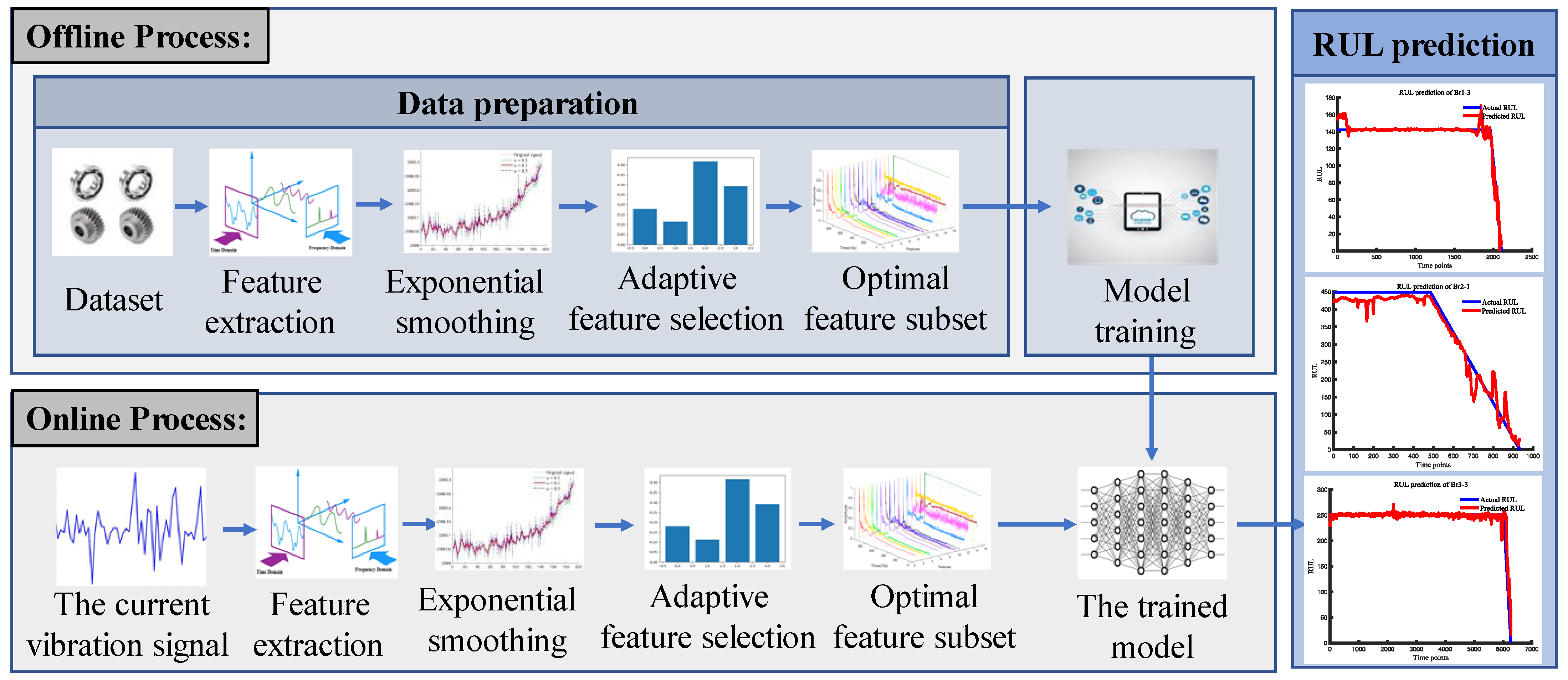
2.1. Data Preprocessing
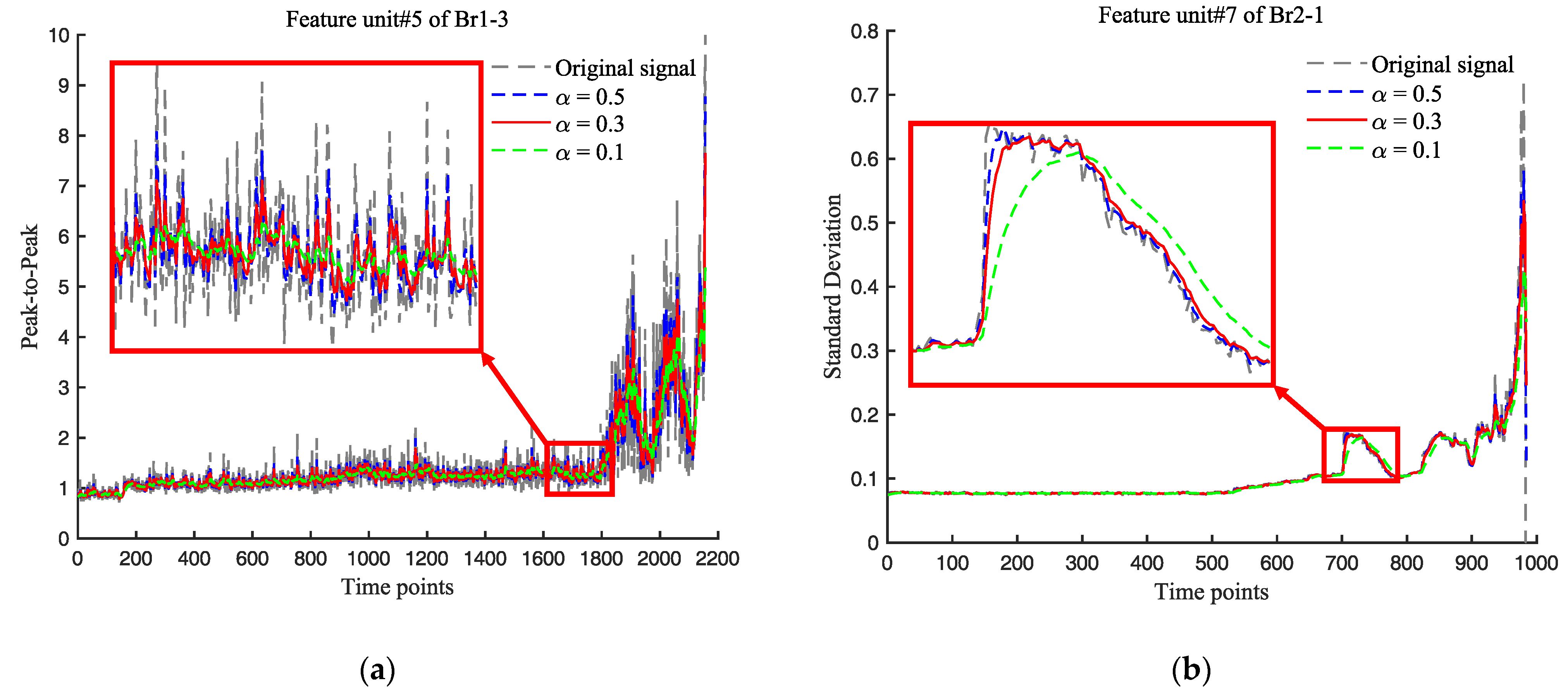
2.1.1. Exponential Smoothing
2.1.2. Adaptive Feature Selection
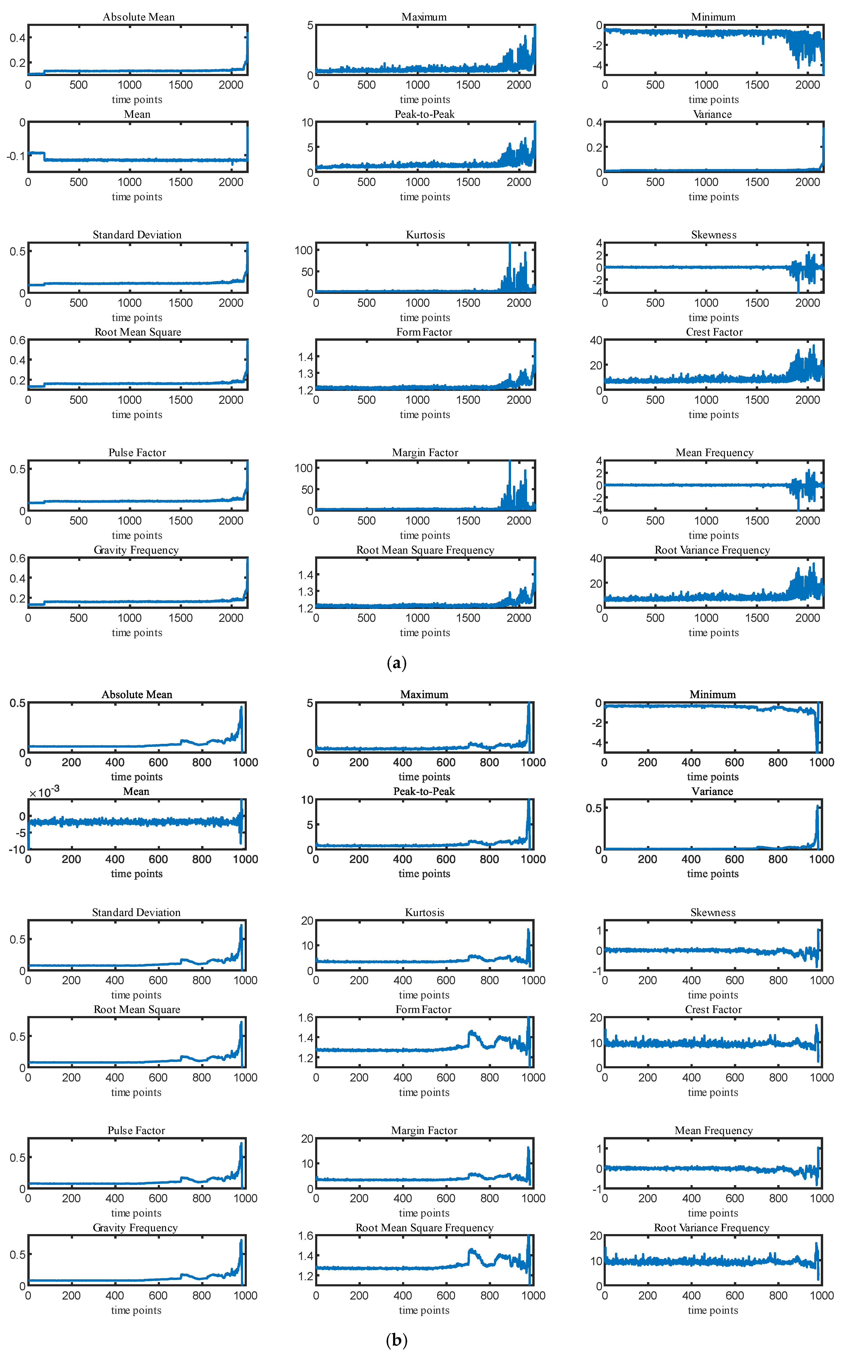
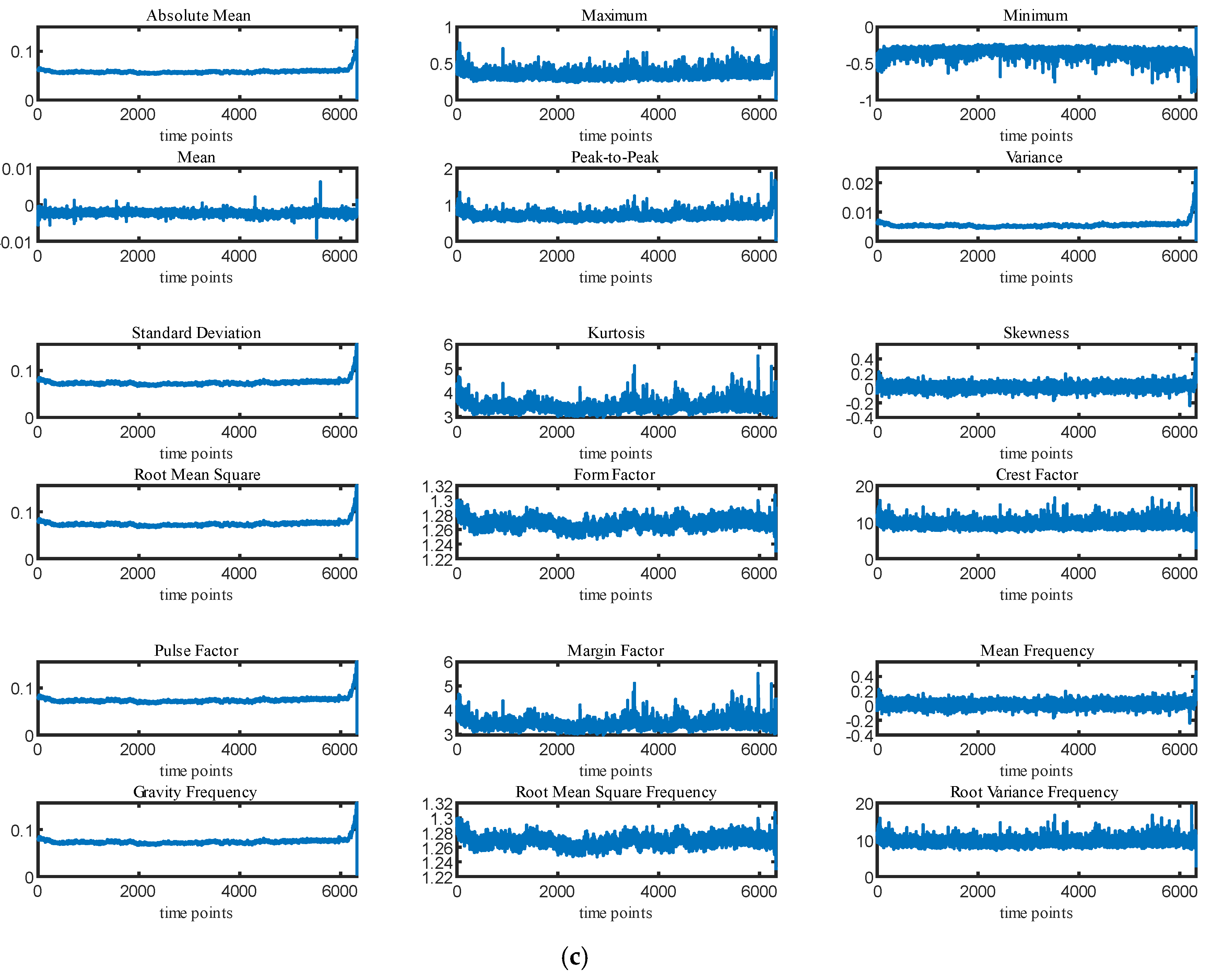
- (I) Feature evaluation indices
- There exists a correlation between the features and the time series of the RUL; features change with the degradation of the equipment.
- Features should be monotonical owing to degradation being an irreversible process.
- Features should have good anti-interference properties against random noise.
- (II) Feature selection
2.1.3. RUL Target Function
2.2. Prediction Model Construction
2.2.1. Basic Theory
- (I) Temporal Convolutional Network
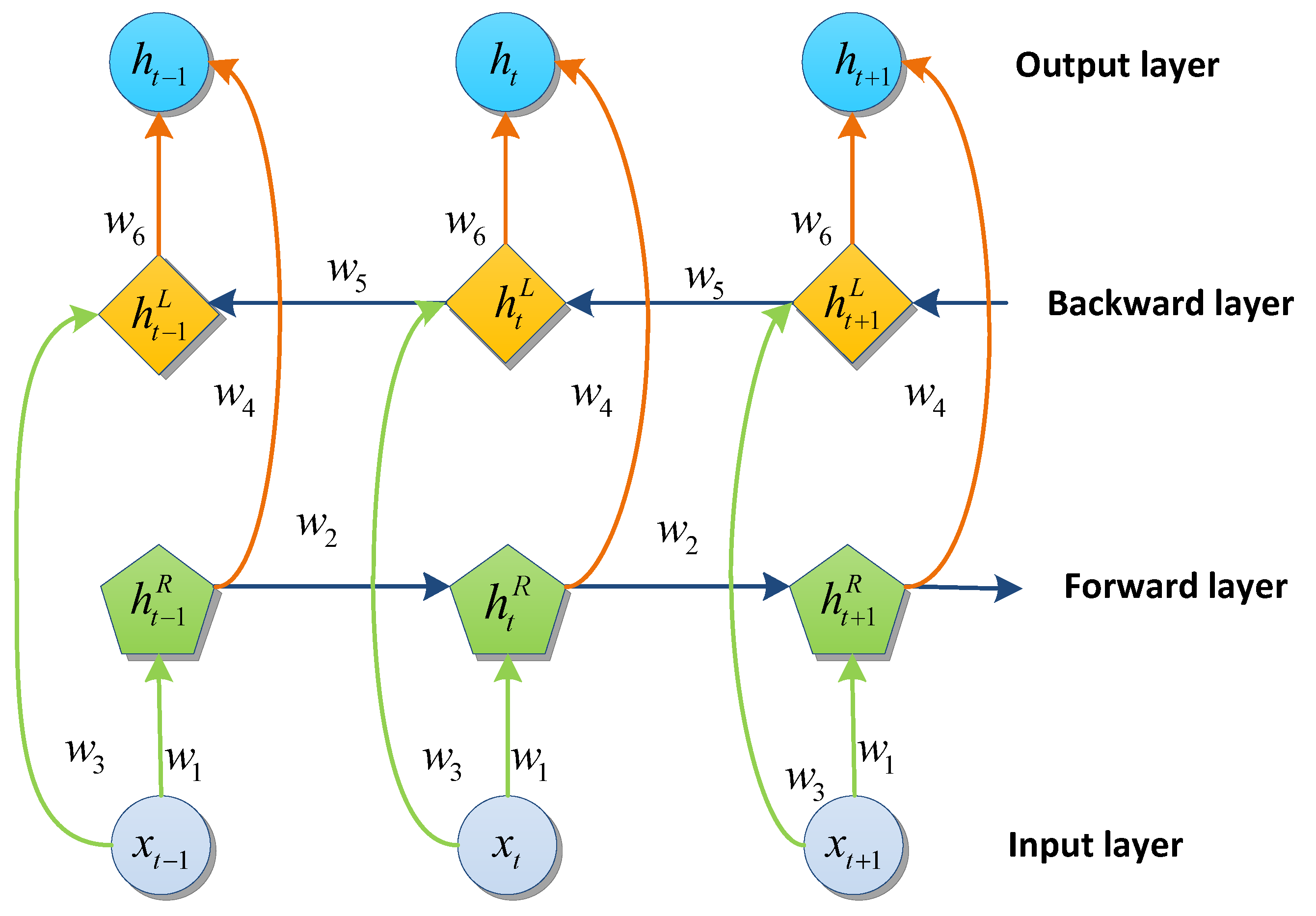
- (II) Bidirectional Long Short-Term Memory
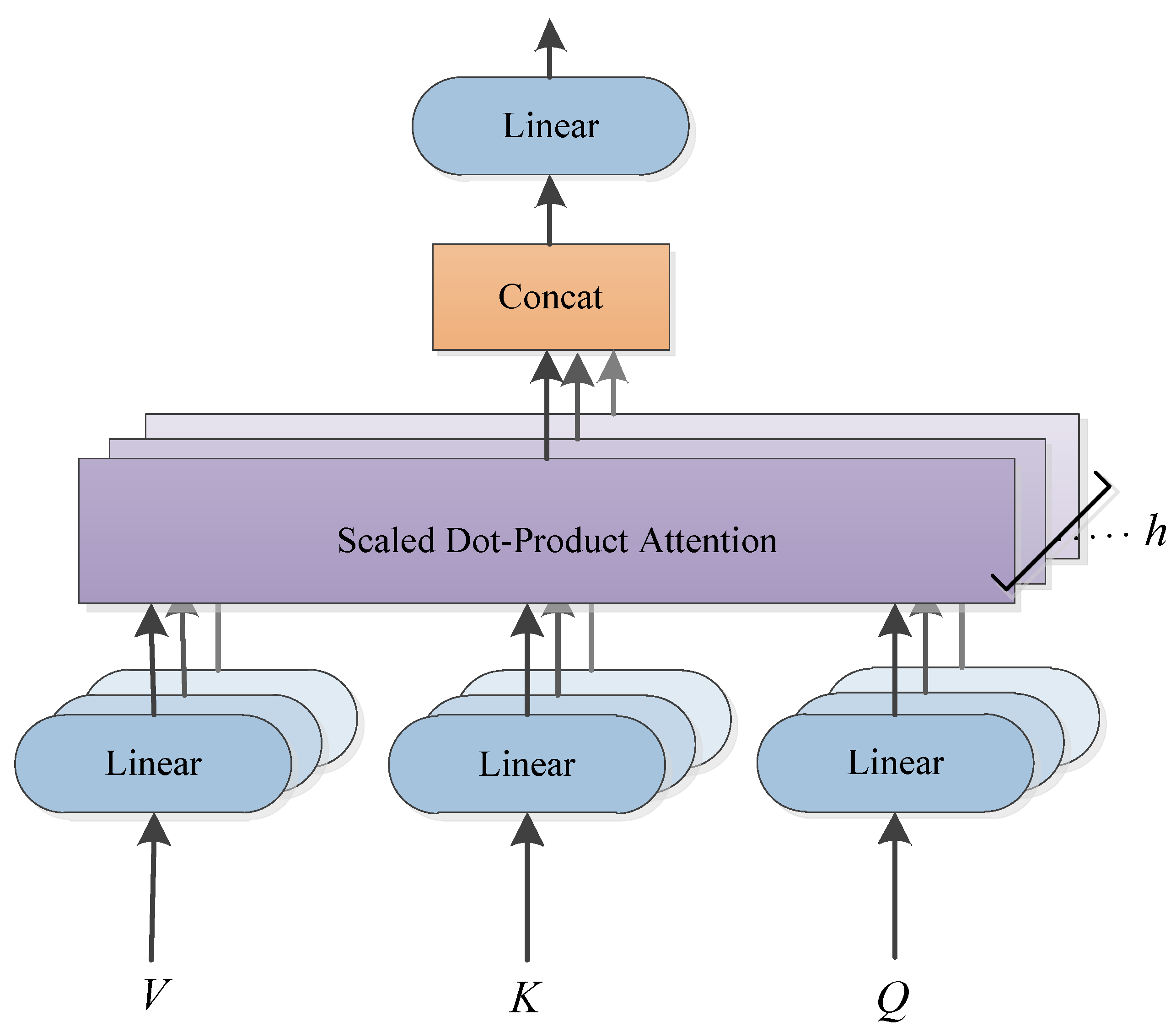
- (III) Multi-head Attention
2.2.2. Metrics
- RMSE: It is a commonly used metric for evaluating prediction models in various fields, including machine learning, statistics, and engineering. It measures the differences between predicted values and actual values by computing the square root of the average squared difference between them. This metric provides a way to quantify the magnitude of the errors in the predictions and can be used to compare the performance of different prediction models.
- MAPE: It is another commonly used evaluation metric for predicting RUL. MAPE measures the percentage difference between predicted values and actual values, which makes it useful for assessing the accuracy of predictions when the scale of the data varies widely.
- SCORE: Early prediction is often more important and effective than later prediction for gradually degrading equipment, such as aircraft engines, bearings, etc., which experience gradual deterioration within their operational life cycle, and their failures typically develop gradually, causing progressive damage to the equipment over a period of time. By setting a penalty for later predictions compared to early predictions, the score function can better capture the preference for early predictions. This is particularly useful for capturing the early warning signs of equipment degradation and preventing catastrophic failures.
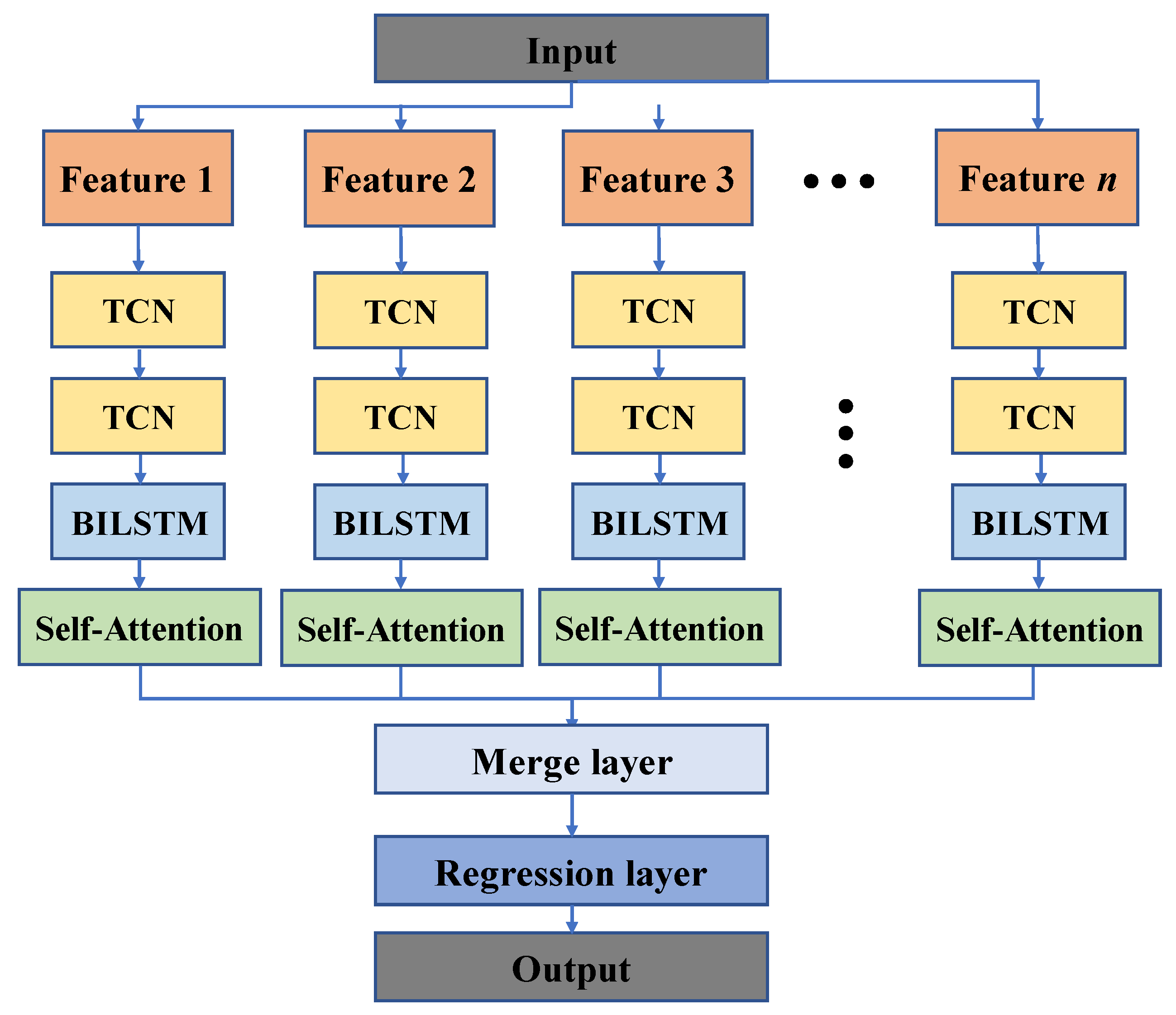
2.2.3. Proposed Model
3. Case Studies
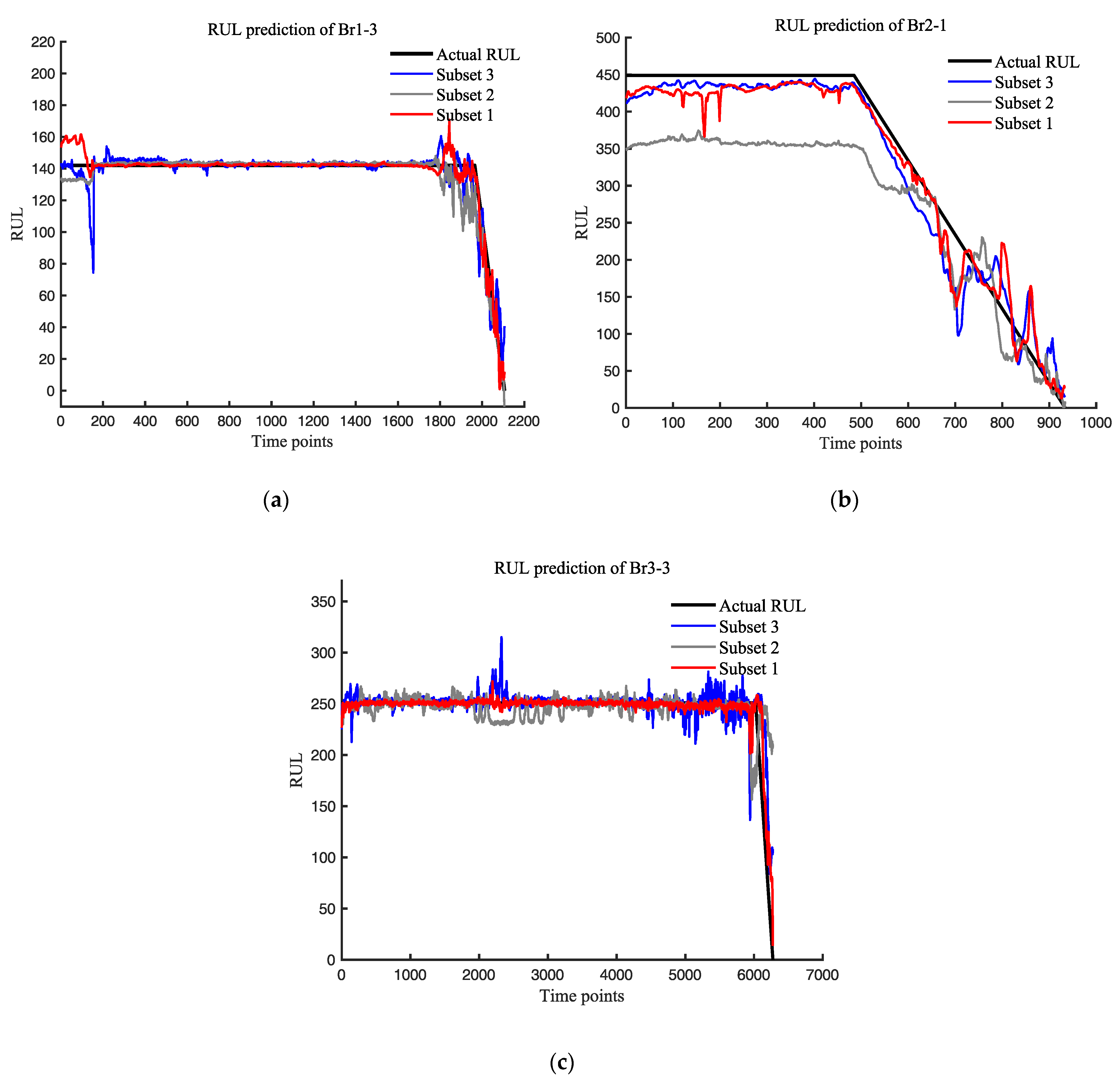
3.1. Case Study1: Intelligent Maintenance System (IMS) Bearing Dataset
3.1.1. Dataset Description
3.1.2. Data Preparation
3.1.3. Optimal Feature Subset
3.1.4. Discussion and Comparison
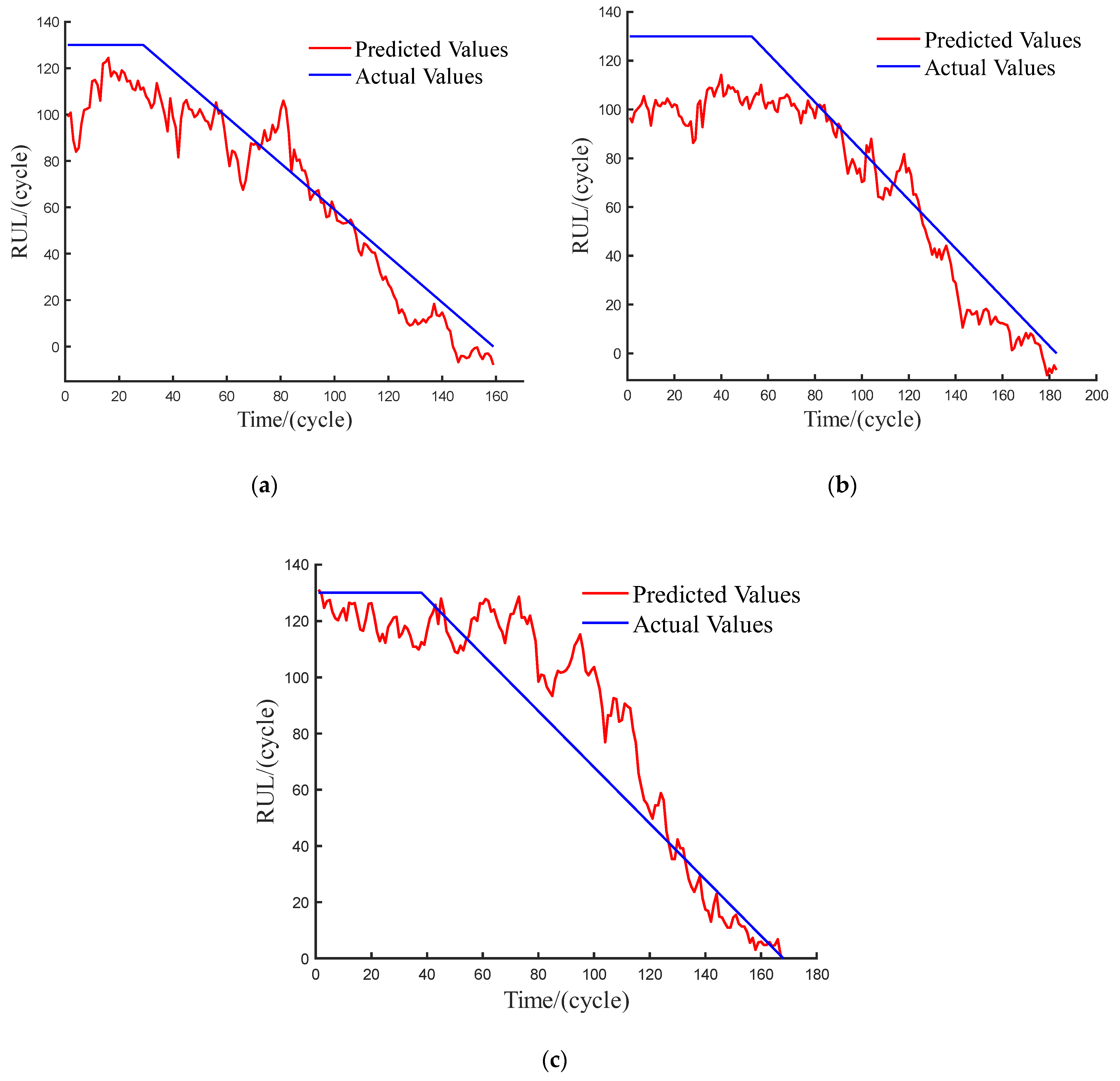
3.2. Case Study2: C-MAPSS Aeroengines Dataset
3.2.1. Dataset Description
3.2.2. Data Preparation
3.2.3. Optimal Feature Subset
3.2.4. Discussion and Comparison
4. Conclusions
Author Contributions
Funding
Data Availability Statement
Conflicts of Interest
References
- Lu, Y.; Li, Q.; Liang, S.Y. Physics-based intelligent prognosis for rolling bearing with fault feature extraction. Int. J. Adv. Manuf. Technol. 2018, 97, 611–620. [Google Scholar] [CrossRef]
- Zhao, H.; Liu, H.; Jin, Y.; Dang, X.; Deng, W. Feature Extraction for Data-Driven Remaining Useful Life Prediction of Rolling Bearings. IEEE Trans. Instrum. Meas. 2021, 70, 3511910. [Google Scholar] [CrossRef]
- Gao, T.; Li, Y.; Huang, X.; Wang, C. Data-Driven Method for Predicting Remaining Useful Life of Bearing Based on Bayesian Theory. Sensors 2021, 21, 182. [Google Scholar] [CrossRef] [PubMed]
- Que, Z.; Jin, X.; Xu, Z. Remaining Useful Life Prediction for Bearings Based on a Gated Recurrent Unit. IEEE Trans. Instrum. Meas. 2021, 70, 3511411. [Google Scholar] [CrossRef]
- Kai, G.; Celaya, J.; Sankararaman, S.; Roychoudhury, I.; Saxena, A. Prognostics: The Science of Making Predictions; CreateSpace Independent Publishing Platform: Scotts Valley, CA, USA, 2017. [Google Scholar]
- Shen, F.; Yan, R. A New Intermediate-Domain SVM-Based Transfer Model for Rolling Bearing RUL Prediction. IEEE/ASME Trans. Mechatron. 2022, 27, 1357–1369. [Google Scholar] [CrossRef]
- Wang, F.; Liu, X.; Liu, C.; Li, H.; Han, Q. Remaining Useful Life Prediction Method of Rolling Bearings Based on Pchip-EEMD-GM(1,1) Model. Shock Vib. 2018, 2018, 3013684. [Google Scholar] [CrossRef]
- Zhu, J.; Chen, N.; Shen, C. A new data-driven transferable remaining useful life prediction approach for bearing under different working conditions. Mech. Syst. Signal Process. 2020, 139, 106602. [Google Scholar] [CrossRef]
- Guo, L.; Li, N.; Jia, F.; Lei, Y.; Lin, J. A recurrent neural network based health indicator for remaining useful life prediction of bearings. Neurocomputing 2017, 240, 98–109. [Google Scholar] [CrossRef]
- Mi, J.; Liu, L.; Zhuang, Y.; Bai, L.; Li, Y.-F. A Synthetic Feature Processing Method for Remaining Useful Life Prediction of Rolling Bearings. IEEE Trans. Reliab. 2022, 72, 125–136. [Google Scholar] [CrossRef]
- Saufi, M.S.R.M.; Hassan, K.A. Remaining useful life prediction using an integrated Laplacian-LSTM network on machinery components. Appl. Soft Comput. 2021, 112, 107817. [Google Scholar] [CrossRef]
- Behera, S.; Misra, R.; Sillitti, A. Multiscale deep bidirectional gated recurrent neural networks based prognostic method for complex non-linear degradation systems. Inf. Sci. 2021, 554, 120–144. [Google Scholar] [CrossRef]
- Zhang, Y.; Xin, Y.; Liu, Z.-W.; Chi, M.; Ma, G. Health status assessment and remaining useful life prediction of aero-engine based on BiGRU and MMoE. Reliab. Eng. Syst. Saf. 2022, 220, 108263. [Google Scholar] [CrossRef]
- Xiang, S.; Qin, Y.; Luo, J.; Pu, H.Y.; Tang, B.P. Multicellular LSTM-based deep learning model for aero-engine remaining useful life prediction. Reliab. Eng. Syst. Saf. 2021, 216, 107927. [Google Scholar] [CrossRef]
- Zhang, N.; Wu, L.; Wang, Z.; Guan, Y. Bearing Remaining Useful Life Prediction Based on Naive Bayes and Weibull Distributions. Entropy 2018, 20, 944. [Google Scholar] [CrossRef] [PubMed] [Green Version]
- Zhang, B.; Zhang, L.; Xu, J. Degradation Feature Selection for Remaining Useful Life Prediction of Rolling Element Bearings. Qual. Reliab. Eng. Int. 2016, 32, 547–554. [Google Scholar] [CrossRef]
- Pan, M.; Hu, P.; Gao, R.; Liang, K. Multistep prediction of remaining useful life of proton exchange membrane fuel cell based on temporal convolutional network. Int. J. Green Energy 2022, 20, 408–422. [Google Scholar] [CrossRef]
- Ding, H.; Yang, L.; Cheng, Z.; Yang, Z. A remaining useful life prediction method for bearing based on deep neural networks. Measurement 2020, 172, 108878. [Google Scholar] [CrossRef]
- Niu, T.; Zhang, L.; Zhang, B.; Yang, B.; Wei, S. An Improved Prediction Model Combining Inverse Exponential Smoothing and Markov Chain. Math. Probl. Eng. 2020, 2020, 6210616. [Google Scholar] [CrossRef]
- Lv, M.; Liu, S.; Su, X.; Chen, C. Early degradation detection of rolling bearing based on adaptive variational mode decomposition and envelope harmonic to noise ratio. J. Vib. Shock 2021, 40, 271–280. [Google Scholar] [CrossRef]
- Cheng, Y.; Wu, J.; Zhu, H.; Or, S.W.; Shao, X. Remaining Useful Life Prognosis Based on Ensemble Long Short-Term Memory Neural Network. IEEE Trans. Instrum. Meas. 2021, 70, 3503912. [Google Scholar] [CrossRef]
- Wu, J.Y.; Min, W.; Chen, Z.; Li, X.L.; Yan, R. Degradation-Aware Remaining Useful Life Prediction With LSTM Autoencoder. IEEE Trans. Instrum. Meas. 2021, 70, 3511810. [Google Scholar] [CrossRef]
- Thakkar, U.; Chaoui, H. Remaining Useful Life Prediction of an Aircraft Turbofan Engine Using Deep Layer Recurrent Neural Networks. Actuators 2022, 11, 67. [Google Scholar] [CrossRef]
- Liao, Y.; Zhang, L.; Liu, C. Uncertainty prediction of remaining useful life using long short-term memory network based on bootstrap method. In Proceedings of the 2018 IEEE International Conference on Prognostics and Health Management (ICPHM), Seattle, WA, USA, 11–13 June 2018; pp. 1–8. [Google Scholar]
- Zhang, C.; Lim, P.; Qin, A.K.; Tan, K.C. Multiobjective Deep Belief Networks Ensemble for Remaining Useful Life Estimation in Prognostics. IEEE Trans. Neural Netw. Learn. Syst. 2017, 28, 2306–2318. [Google Scholar] [CrossRef] [PubMed]
- Shuai, Z.; Ristovski, K.; Farahat, A.; Gupta, C. Long Short-Term Memory Network for Remaining Useful Life estimation. In Proceedings of the 2017 IEEE International Conference on Prognostics and Health Management (ICPHM), Dallas, TX, USA, 19–21 June 2017. [Google Scholar]
- Sateesh Babu, G.; Zhao, P.; Li, X.-L. Deep Convolutional Neural Network Based Regression Approach for Estimation of Remaining Useful Life. In Proceedings of the Database Systems for Advanced Applications, Cham, Switzerland, 25 March 2016; pp. 214–228. [Google Scholar]
- Gu, Y.; Wylie, B.K.; Boyte, S.P.; Picotte, J.; Howard, D.M.; Smith, K.; Nelson, K.J. An Optimal Sample Data Usage Strategy to Minimize Overfitting and Underfitting Effects in Regression Tree Models Based on Remotely-Sensed Data. Remote Sens. 2016, 8, 943. [Google Scholar] [CrossRef] [Green Version]


| Type | Definition |
|---|---|
| Input Layer | The input layer |
| TCN | filters = 32, kernel size = 3 |
| Batch Norm | Batch normalization |
| TCN | filters = 32, kernel size = 3 |
| Batch Norm | Batch normalization |
| Bidirectional(LSTM) | Units = 32 |
| Batch Norm | Batch normalization |
| SeqSelfAttention | Self-attentional layer |
| MaxPooling1D | The pooling layer |
| Flatten | Returns a 1D array |
| Concatenate | Merge the channels |
| Dense | Dense to 50 |
| Dense | Dense to 1 |
| Test Number | File Number | Fault Bearing | Symbol | Fault Bearing |
|---|---|---|---|---|
| Test 1 | 2156 | Bearing 3 | Br1-3 | inner race |
| Test 2 | 984 | Bearing 1 | Br2-1 | outer race |
| Test 3 | 6324 | Bearing 3 | Br3-3 | outer race |
| Bearings | α | RMSE | SCORE | MAPE |
|---|---|---|---|---|
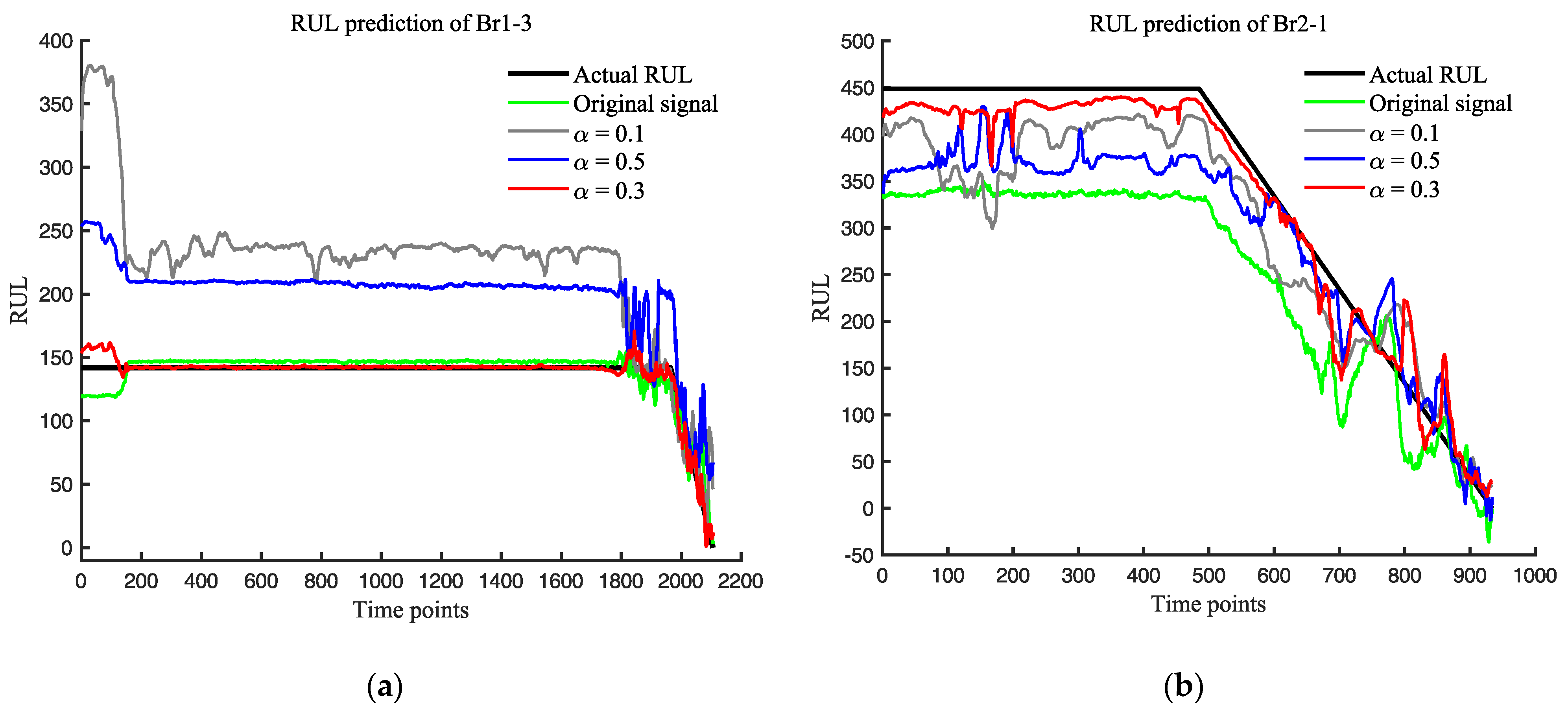
| Br1-3 | 0 | 9.30 | 3.55 × 10³ | 0.07 |
| 0.1 | 99.85 | 1.42 × 10¹² | 0.74 | |
| 0.3 | 5.28 | 9.34 × 10² | 0.03 | |
| 0.5 | 66.28 | 8.45 × 10⁶ | 0.56 | |
| Br2-1 | 0 | 99.13 | 4.34 × 10⁶ | 0.36 |
| 0.1 | 56.41 | 1.27 × 10⁶ | 0.23 | |
| 0.3 | 26.18 | 1.22 × 10⁵ | 0.15 | |
| 0.5 | 62.36 | 3.46 × 10⁵ | 0.19 | |
| Br3-3 | 0 | 25.61 | 8.01 × 10⁹ | 0.17 |
| 0.1 | 14.41 | 2.40 × 10⁵ | 0.04 | |
| 0.3 | 10.83 | 1.23 × 10⁵ | 0.05 | |
| 0.5 | 11.45 | 1.65 × 10⁵ | 0.05 |
| Bearings | Corr | Mon | Rob |
|---|---|---|---|
| Br1-3 | 8.46 | 39.34 | 8.28 |
| Br2-1 | 5.33 | 13.11 | 9.31 |
| Br3-3 | 5.17 | 29.93 | 10.16 |
| Feature Subsets | Features |
|---|---|
| Subset 1 | 1,10,4,15,6,7,5,8,2,3,9 |
| Subset 2 | 1–18 |
| Subset 3 | 1,10,7,15,16,18,6,3,17,5,14 |
| Bearings | Subset | RMSE | SCORE | MAPE |
|---|---|---|---|---|
| Br1-3 | 1 | 5.28 | 9.34 × 10² | 0.03 |
| 2 | 7.13 | 1.33 × 10³ | 0.04 | |
| 3 | 8.25 | 2.63 × 10³ | 0.07 | |
| Br2-1 | 1 | 26.18 | 1.22 × 10⁵ | 0.15 |
| 2 | 74.07 | 6.44 × 10⁵ | 0.21 | |
| 3 | 31.11 | 1.74 × 10⁴ | 0.19 | |
| Br3-3 | 1 | 10.83 | 1.23 × 10⁵ | 0.05 |
| 2 | 27.55 | 1.34 × 10¹⁰ | 0.19 | |
| 3 | 17.85 | 3.38 × 10⁶ | 0.10 |
| Bearings | Model | RMSE | SCORE | MAPE |
|---|---|---|---|---|
| Br1-3 | TCN | 17.51 | 1.17 × 10⁵ | 0.11 |
| CNN | 21.06 | 6.61 × 10⁵ | 0.07 | |
| LSTM | 20.06 | 9.68 × 10⁴ | 0.12 | |
| BILSTM | 30.05 | 3.03 × 10⁶ | 0.23 | |
| BIGRU | 34.24 | 4.06 × 10⁷ | 0.26 | |
| CNN-LSTM | 18.47 | 2.54 × 10⁴ | 0.19 | |
| TCN-BIGRU | 28.27 | 7.41 × 10⁶ | 0.11 | |
| TCN-BILSTM | 16.93 | 5.12 × 10⁴ | 0.08 | |
| Proposed model | 5.28 | 9.34 × 10² | 0.03 | |
| Br2-1 | TCN | 45.63 | 5.24 × 10⁶ | 0.42 |
| CNN | 28.48 | 1.07 × 10⁵ | 0.25 | |
| LSTM | 52.98 | 1.28 × 10⁹ | 0.22 | |
| BILSTM | 61.66 | 1.98 × 10⁸ | 0.36 | |
| BIGRU | 40.48 | 1.91 × 10⁶ | 0.22 | |
| CNN-LSTM | 44.93 | 9.44 × 10⁶ | 0.34 | |
| TCN-BIGRU | 36.31 | 3.53 × 10⁵ | 0.14 | |
| TCN-BILSTM | 29.62 | 4.16 × 10⁵ | 0.12 | |
| Proposed model | 26.18 | 1.22 × 10⁵ | 0.15 | |
| Br3-3 | TCN | 20.59 | 5.81 × 10⁹ | 0.19 |
| CNN | 16.06 | 2.51 × 10⁸ | 0.13 | |
| LSTM | 11.64 | 8.09 × 10⁴ | 0.04 | |
| BILSTM | 13.24 | 1.56 × 10⁴ | 0.08 | |
| BIGRU | 29.75 | 1.18 × 10¹³ | 0.22 | |
| CNN-LSTM | 12.49 | 2.48 × 10⁵ | 0.06 | |
| TCN-BIGRU | 12.06 | 1.00 × 10⁵ | 0.07 | |
| TCN-BILSTM | 11.66 | 1.28 × 10⁵ | 0.07 | |
| Proposed model | 10.83 | 1.23 × 10⁵ | 0.05 |
| Dataset | FD001 | |
|---|---|---|
| Training Set | Testing Set | |
| Engines | 100 | 100 |
| Sensor measurements | 21 | 21 |
| Operation conditions | H = 0 kft Ma = 0 TRA = 100° | |
| Fault modes | Fault of high-pressure compressor | |
| No. | Symbol | Description | Units |
|---|---|---|---|
| 1 | T2 | Total temperature at fan inlet | (°) |
| 2 | T24 | Total temperature at LPC outlet | (°) |
| 3 | T30 | Total temperature at HPC outlet | (°) |
| 4 | T50 | Total temperature at LPT outlet | (°) |
| 5 | P2 | Pressure at fan inlet | Pa |
| 6 | P15 | Total pressure in bypass-duct | Pa |
| 7 | P30 | Total pressure at HPC outlet | Pa |
| 8 | Nf | Physical fan speed | r/min |
| 9 | Nc | Physical core speed | r/min |
| 10 | epr | Engine pressure ratio (P50/P2) | - |
| 11 | Ps30 | Static pressure at HPC outlet | Pa |
| 12 | Phi | Ratio of fuel flow to Ps30 | pps/psi |
| 13 | NRf | Corrected fan speed | r/min |
| 14 | NRc | Corrected core speed | r/min |
| 15 | BPR | Bypass ratio | - |
| 16 | FarB | Burner fuel–air ratio | - |
| 17 | htBleed | Bleed enthalpy | - |
| 18 | Nf_dmd | Demanded fan speed | r/min |
| 19 | PCNfR_dmd | Demanded corrected fan speed | r/min |
| 20 | W31 | HPT coolant bleed | lbm/s |
| 21 | W32 | LPT coolant bleed | lbm/s |
| Feature Subsets | Features |
|---|---|
| Subset 1 | 2,3,4,7,8,9,11,12,13,15,20,21 |
| Subset 2 | 4,7,8,9,11,12,13,14,15,17,20,21 |
| Subset 3 | 1–21 |
| Subset | RMSE | SCORE |
|---|---|---|
| 1 | 13.99 | 313 |
| 2 | 15.42 | 411 |
| 3 | 17.85 | 969 |
Disclaimer/Publisher’s Note: The statements, opinions and data contained in all publications are solely those of the individual author(s) and contributor(s) and not of MDPI and/or the editor(s). MDPI and/or the editor(s) disclaim responsibility for any injury to people or property resulting from any ideas, methods, instructions or products referred to in the content. |
© 2023 by the authors. Licensee MDPI, Basel, Switzerland. This article is an open access article distributed under the terms and conditions of the Creative Commons Attribution (CC BY) license (https://creativecommons.org/licenses/by/4.0/).
Share and Cite
Nie, L.; Xu, S.; Zhang, L. Multi-Head Attention Network with Adaptive Feature Selection for RUL Predictions of Gradually Degrading Equipment. Actuators 2023, 12, 158. https://doi.org/10.3390/act12040158
Nie L, Xu S, Zhang L. Multi-Head Attention Network with Adaptive Feature Selection for RUL Predictions of Gradually Degrading Equipment. Actuators. 2023; 12(4):158. https://doi.org/10.3390/act12040158
Chicago/Turabian StyleNie, Lei, Shiyi Xu, and Lvfan Zhang. 2023. "Multi-Head Attention Network with Adaptive Feature Selection for RUL Predictions of Gradually Degrading Equipment" Actuators 12, no. 4: 158. https://doi.org/10.3390/act12040158