
Improved Craig–Bampton Method Implemented into Durability Analysis of Flexible Multibody Systems
Abstract
:1. Introduction
2. Small Deformation Theory of Floating Frame of Reference Formulation
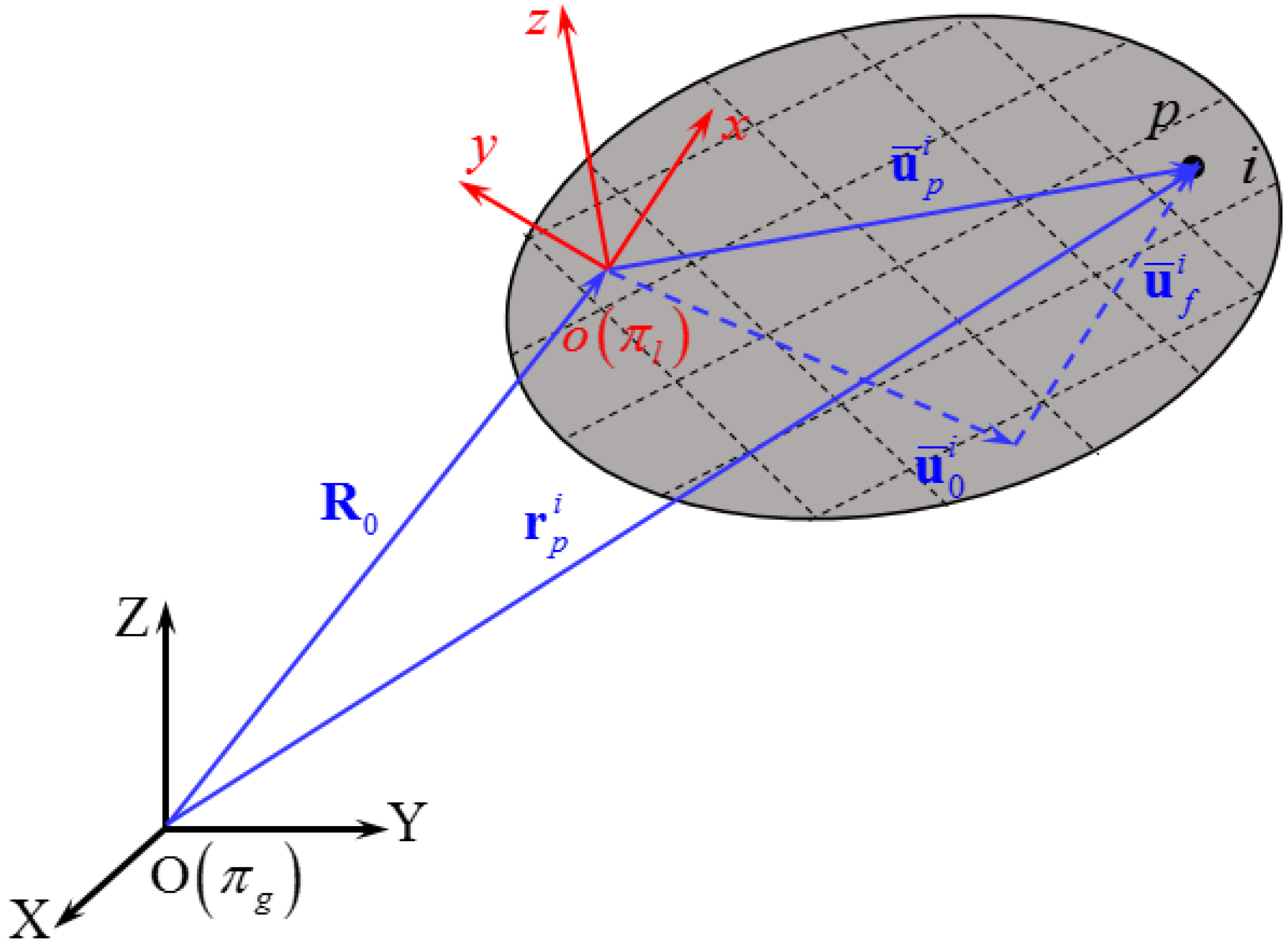
2.1. Position Equation of an Arbitrary Point on the Flexible Body
2.2. Equation of Motion of the Flexible Multibody System
3. Orthogonal Craig–Bampton Modal Transformation Matrix
3.1. Component Mode Synthesis (Normal Mode Approach)
3.2. Craig–Bampton Modal Transformation Matrix
3.2.1. Static Correction Modes
3.2.2. Fixed Interface Modes
3.2.3. Original CB Modal Transformation Matrix
3.2.4. Orthogonal CB Modal Transformation Matrix
4. Applied Limitation of the Free-Free Modes
5. Improved Craig–Bampton Modal Transformation Matrix
5.1. Imposing the Reference Conditions on the Original CB Matrix
5.2. Imposing Reference Conditions Prior to Forming the Craig–Bampton Matrix
6. Conclusions
- (1)
- The CB method only generates the free-free modes; however, the free-free modes can lead to the wrong solution in some scenarios, as was demonstrated in this paper by a simple planar beam example. If the CB method is to be used for many applications, reference conditions must be imposed to improve the CB method. In this paper, two different methods are proposed to improve the CB method. The first method is to directly impose the reference condition on the unit matrix of the original CB matrix. The second method is to impose the reference conditions on the shape functions to calculate the new mass and stiffness matrices; subsequently, the improved CB matrix can be derived from the new mass and stiffness matrices. Although these two different methods are adopted to improve the CB matrix to make it suitable for all applications, the simulation results from both methods in the durability analysis are the same.
- (2)
- The CB method is not only used to derive the free-free modes but can be suited for deriving the simply-supported modes (or other modes, such as pinned-pinned, fixed-fixed, fixed-free, etc.) only if the appropriate reference conditions are imposed on the original CB matrix or on the shape functions prior to forming the improved CB matrix. Otherwise, the wrong solution will be obtained in some special cases, and it may be difficult to determine the reasons that lead to the wrong solution. Hence, the reference condition concept should be paid more attention to prior to implementing the static or dynamic analysis of the flexible multibody systems. The application area of the CB method is thus expanded from only free-free modes to any other mode.
- (3)
- Although the normal mode approach is a more direct method to obtain the normal modes compared to the improved CB method, the improved CB method has a much clearer physical meaning compared to the normal mode approach. The topology structure and constraint information of the flexible multibody system can be directly obtained from the CB modal transformation matrix, which is better than the generalized normal mode approach. In addition, it is very convenient to impose the reference conditions on the original CB modal transformation matrix or shape functions; hence, the structure of the improved CB method is beneficial for programming code during the durability analysis of the flexible multibody system so as to improve computational efficiency.
Author Contributions
Funding
Conflicts of Interest
References
- Masson, G.; Brik, B.A.; Cogan, S.; Bouhaddi, N. Component mode synthesis (CMS) based on an enriched ritz approach for efficient structural optimization. J. Sound Vib. 2006, 296, 845–860. [Google Scholar] [CrossRef]
- Hu, H.; Lin, Y.; Hu, Y. Synthesis, structures and applications of single component core-shell structured TiO2: A review. Chem. Eng. J. 2019, 375, 122029. [Google Scholar] [CrossRef]
- Corradi, G.; Sinou, J.; Besset, S. Performances of the double modal synthesis for the prediction of the transient self-sustained vibration and squeal noise. Appl. Acoust. 2021, 175, 107807. [Google Scholar] [CrossRef]
- Yotov, V.V.; Remedia, M.; Aglietti, G.; Richardson, G. Improved Craig–Bampton stochastic method for spacecraft vibroacoustic analysis. Acta Astronaut. 2021, 178, 556–570. [Google Scholar] [CrossRef]
- Tian, W.; Gu, Y.; Liu, H.; Wang, X.; Yang, Z.; Li, Y.; Li, P. Nonlinear aeroservoelastic analysis of a supersonic aircraft with control fin free-play by component mode synthesis technique. J. Sound Vib. 2021, 493, 115835. [Google Scholar] [CrossRef]
- Kim, J.; Kim, J.; Lee, P. Improving the accuracy of the dual Craig-Bampton method. Comput. Struct. 2017, 191, 22–32. [Google Scholar] [CrossRef]
- Yuan, J.; Salles, L.; El Haddad, F.; Wong, C. An adaptive component mode synthesis method for dynamic analysis of jointed structure with contact friction interfaces. Comput. Struct. 2020, 229, 106177. [Google Scholar] [CrossRef]
- Cui, J.; Zheng, G. An iterative state-space component modal synthesis approach for damped systems. Mech. Syst. Signal Process. 2020, 142, 106558. [Google Scholar] [CrossRef]
- Bai, B.; Li, H.; Zhang, W.; Cui, Y. Application of extremum response surface method-based improved substructure component modal synthesis in mistuned turbine bladed disk. J. Sound Vib. 2020, 472, 115210. [Google Scholar] [CrossRef]
- Nowakowski, C.; Fehr, J.; Fischer, M.; Eberhard, P. Model order reduction in elastic multibody systems using the floating frame of reference formulation. IFAC Proc. 2012, 45, 40–48. [Google Scholar] [CrossRef]
- Canavin, J.; Likins, P. Floating Reference Frames for Flexible Spacecraft. J. Spacecr. Rocket. 1977, 14, 724–732. [Google Scholar] [CrossRef]
- García-Vallejo, D.; Sugiyama, H.; Shabana, A. Finite element analysis of the geometric stiffening effect. Part 1: A correction in the floating frame of reference formulation. Proc. Inst. Mech. Eng. Part K J. Multi-Body Dyn. 2005, 219, 187–202. [Google Scholar] [CrossRef]
- Shabana, A.; Wang, G. Durability analysis and implementation of the floating frame of reference formulation. Proc. Inst. Mech. Eng. Part K J. Multi-Body Dyn. 2018, 232, 295–313. [Google Scholar] [CrossRef]
- Krattiger, D.; Wu, L.; Zacharczuk, M.; Buck, M.; Kuether, R.; Allen, M.; Tiso, P.; Brake, M. Interface reduction for Hurty/Craig-Bampton substructured models: Review and improvements. Mech. Syst. Signal Process. 2019, 114, 579–603. [Google Scholar] [CrossRef]
- Wang, T.; He, J.; Hou, S.; Deng, X.; Xi, C.; He, H. Complex component mode synthesis method using hybrid coordinates for generally damped systems with local nonlinearities. J. Sound Vib. 2020, 476, 115299. [Google Scholar] [CrossRef]
- Jezequel, L.; Seito, H. Component modal synthesis methods based on hybrid models, Part I: Theory of hybrid models and modal truncation methods. J. Appl. Mech. Trans. ASME 1994, 61, 100–108. [Google Scholar] [CrossRef]
- Miraglia, G.; Petrovic, M.; Abbiati, G.; Mojsilovic, N.; Stojadinovic, B. A model-order reduction framework for hybrid simulation based on component-mode synthesis. Earthq. Eng. Struct. Dyn. 2020, 49, 737–753. [Google Scholar] [CrossRef]
- Spanos, J.T.; Tsuha, W.S. Selection of deformation modes for flexible multibody simulation. J. Guid. 1991, 14, 278–286. [Google Scholar] [CrossRef]
- Hurty, W. Dynamic Analysis of Structural Systems Using Component Modes. AIAA J. 1965, 3, 678–685. [Google Scholar] [CrossRef]
- Gladwell, G. Branch mode analysis of vibrating systems. J. Sound Vib. 1964, 1, 41–59. [Google Scholar] [CrossRef]
- Rubin, S. Improved Component-Mode Representation for Structural Dynamic Analysis. AIAA J. 1975, 13, 995–1006. [Google Scholar] [CrossRef]
- Shabana, A.; Wang, G.; Kulkarni, S. Further investigation on the coupling between the reference and elastic displacements in flexible body dynamics. J. Sound Vib. 2018, 427, 159–177. [Google Scholar] [CrossRef]
- Kuran, B.; Özgüven, H. A modal superposition method for non-linear structures. J. Sound Vib. 1996, 189, 315–339. [Google Scholar] [CrossRef]
- Craig, R. Substructure Methods in Vibration. J. Vib. Acoust. 1995, 117, 207–213. [Google Scholar] [CrossRef]
- JLim, H.; Hwang, D.; Kim, K.; Lee, G.; Kim, J. A coupled dynamic loads analysis of satellites with an enhanced Craig–Bampton approach. Aerosp. Sci. Technol. 2017, 69, 114–122. [Google Scholar] [CrossRef]
- Hinke, L.; Dohnal, F.; Mace, B.; Waters, T.; Ferguson, N. Component mode synthesis as a framework for uncertainty analysis. J. Sound Vib. 2009, 324, 161–178. [Google Scholar] [CrossRef]
- O’Shea, J.; Jayakumar, P.; Mechergui, D.; Shabana, A.; Wang, L. Reference Conditions and Substructuring Techniques in Flexible Multibody System Dynamics. J. Comput. Nonlinear Dyn. 2018, 13, 041007. [Google Scholar] [CrossRef]
- Qiu, J.; Williams, F.; Qiu, R. A new exact substructure method using mixed modes. J. Sound Vib. 2003, 266, 737–757. [Google Scholar] [CrossRef]
- Craig, R.R., Jr.; Bampton, M.C. Coupling of Substructures for Dynamic Analyses. AIAA J. 1968, 6, 1313–1319. [Google Scholar] [CrossRef]
- Junge, M.; Brunner, D.; Becker, J.; Gaul, L. Interface-reduction for the Craig–Bampton and Rubin method applied to FE–BE coupling with a large fluid–structure interface. Int. J. Numer. Methods Eng. 2009, 77, 1731–1752. [Google Scholar]
- Craig, R.R., Jr. Substructure Methods in Vibration. Trans. ASME Spec. 50th Anniv. Des. Issue 1995, 117, 207–213. [Google Scholar]
- Boo, S.-H.; Kim, J.-H.; Lee, P.-S. Towards improving the enhanced Craig-Bampton method. Comput. Struct. 2018, 196, 63–75. [Google Scholar] [CrossRef]
- Gruber, F.; Tim, B.; Rixen, D. Dual Craig-Bampton Method with Reduction of Interface Coordinates. In Proceedings of the IMAC, A Conference and Exposition on Structural Dynamics, Garden Grove, CA, USA, 29 March 2017; Springer International Publishing: Berlin/Heidelberg, Germany, 2017; pp. 1–19. [Google Scholar]
- Kim, J.; Lee, P. An enhanced Craig-Bampton method. Int. J. Numer. Methods Eng. 2015, 103, 79–93. [Google Scholar]
- Rixen, D. A dual Craig-Bampton method for dynamic substructuring. J. Comput. Appl. Math. 2004, 168, 383–391. [Google Scholar] [CrossRef]
- Kim, J.; Lee, K.; Lee, P. Estimating relative eigenvalue errors in the Craig-Bampton method. Comput. Struct. 2014, 139, 54–64. [Google Scholar] [CrossRef]
- Kuether, R.; Allen, M. Craig-Bampton Substructuring for Geometrically Nonlinear Subcomponents. In Dynamics of Coupled Structures; Springer International Publishing: Berlin/Heidelberg, Germany, 2014; Volume 1, pp. 167–178. [Google Scholar]
- Kim, J.; Boo, S.-H.; Lee, P. Performance of the enhanced Craig-Bampton method. In Structural Engineering And Mechanics; Wiley: Hoboken, NJ, USA, 2015; pp. 1–7. [Google Scholar]
- Carassale, L.; Maurici, M. Interface Reduction in Craig-Bampton Component Mode Synthesis by Orthogonal Polynomial Series. In Proceedings of the Turbomachinery Technical Conference & Exposition, Charlotte, NC, USA, 26–30 June 2017; pp. 1–11. [Google Scholar]
- Cammarata, A.; Pappalardo, C. On the use of component mode synthesis methods for the model reduction of flexible multibody systems within the floating frame of reference formulation. Mech. Syst. Signal Process. 2020, 142, 106745. [Google Scholar] [CrossRef]
- Fang, M.; Wang, J.; Liu, H. An adaptive numerical scheme based on the Craig–Bampton method for the dynamic analysis of tall buildings. Struct. Des. Tall Spec Build. 2017, 7, e1410. [Google Scholar] [CrossRef]
- Wang, G.; Wang, L. Coupling relationship of the non-ideal parallel mechanism using modified Craig-Bampton method. Mech. Syst. Signal Process. 2020, 141, 106471. [Google Scholar] [CrossRef]
- Rahnejat, H. Multi-body dynamics: Historical evolution and application. Proc. Inst. Mech. Eng. Part C J. Mech. Eng. Sci. 2000, 214, 149–173. [Google Scholar] [CrossRef]
- Shabana, A. Flexible Multibody Dynamics: Review of Past and Recent Developments. Multibody Syst. Dyn. 1997, 1, 189–222. [Google Scholar] [CrossRef]
- Shabana, A. Dynamics of Multibody Systems; Cambridge University Press: Cambridge, UK, 2013. [Google Scholar] [CrossRef]
- Omar, M.; Shabana, A. A two-dimensional shear deformable beam for large rotation and deformation problems. J. Sound Vib. 2001, 243, 565–576. [Google Scholar] [CrossRef]
- Boo, S.-H.; Lee, P. A dynamic condensation method using algebraic substructuring. Int. J. Numer. Methods Eng. 2017, 109, 1701–1720. [Google Scholar]
- MSC Software, Adams.Flex. 2009. Available online: http://www.mscsoftware.co.kr/upfile/pro_pdf/ADAMS%20Flex_EE_R9.pdf (accessed on 8 January 2023).
- Boo, S.; Lee, P. An iterative algebraic dynamic condensation method and its performance. Comput. Struct. 2017, 182, 419–429. [Google Scholar] [CrossRef]


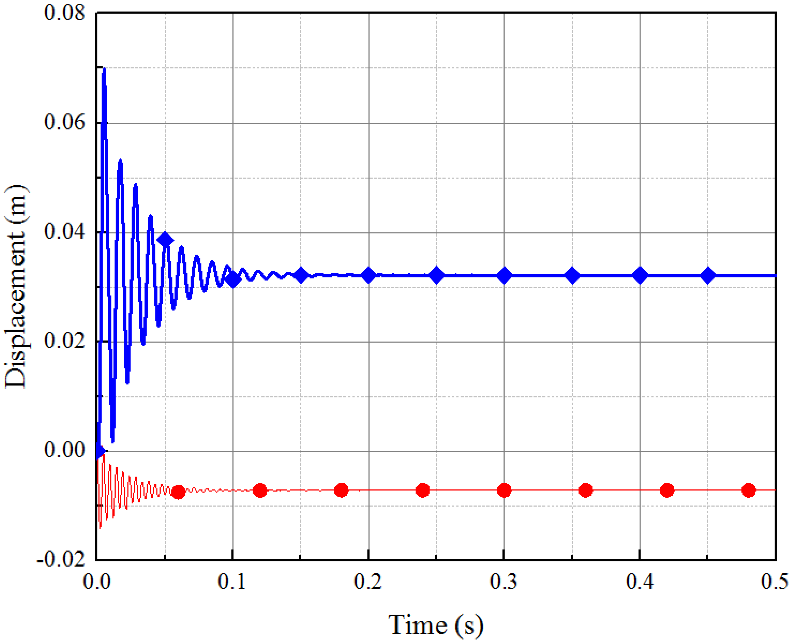
 CB method (free-free modes) and
  ANSYS (simply-supported modes)).
CB method (free-free modes) and ANSYS (simply-supported modes)).
ANSYS (simply-supported modes)).
CB method (free-free modes) and ANSYS (simply-supported modes)).
 CB method (free-free modes) and
  ANSYS (simply-supported modes)).
CB method (free-free modes) and ANSYS (simply-supported modes)).
ANSYS (simply-supported modes)).
CB method (free-free modes) and ANSYS (simply-supported modes)).
 CB method (free-free modes) and
  ANSYS (simply-supported modes)).
CB method (free-free modes) and ANSYS (simply-supported modes)).
ANSYS (simply-supported modes)).
CB method (free-free modes) and ANSYS (simply-supported modes)).
 CB method (free-free modes) and
  ANSYS (simply-supported modes)).
CB method (free-free modes) and ANSYS (simply-supported modes)).
ANSYS (simply-supported modes)).
CB method (free-free modes) and ANSYS (simply-supported modes)).
 CB method (free-free modes) and
  ANSYS (simply-supported modes)).
CB method (free-free modes) and ANSYS (simply-supported modes)).
ANSYS (simply-supported modes)).
CB method (free-free modes) and ANSYS (simply-supported modes)).
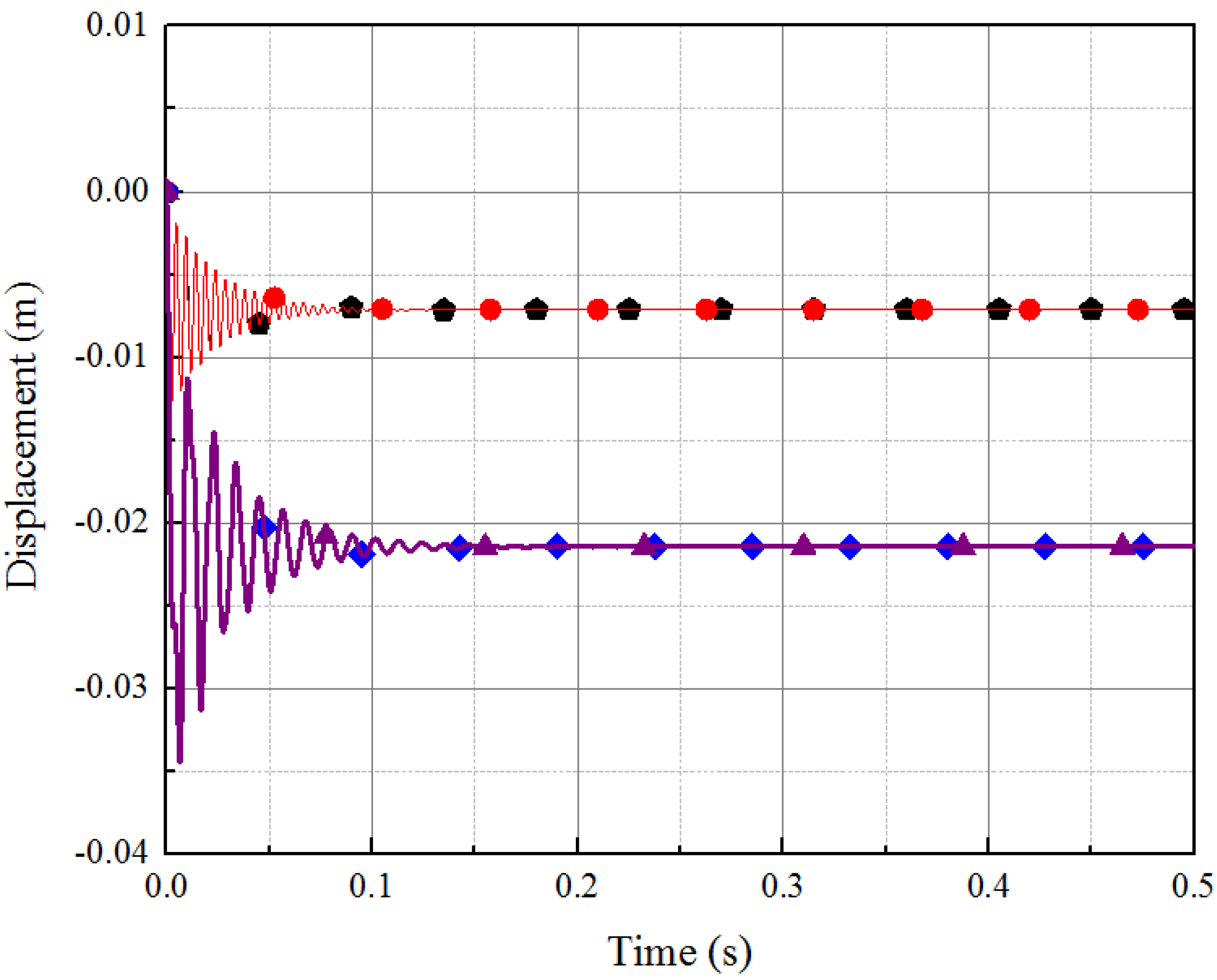
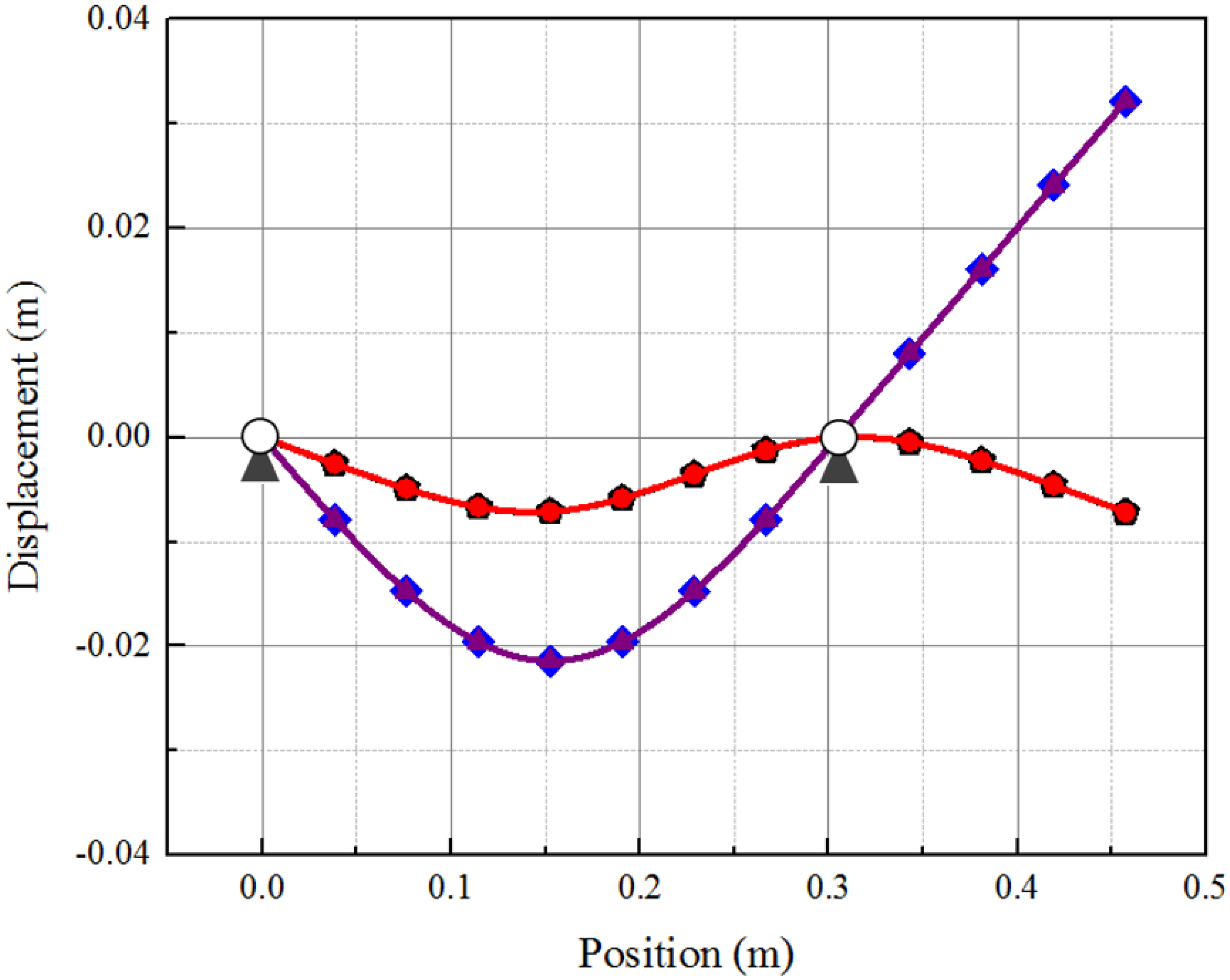
 Normal mode approach (free-free modes),
  CB matrix (free-free modes),
  ANSYS (simply-supported modes), and
  Improved CB matrix (simply-supported modes)).
Normal mode approach (free-free modes), CB matrix (free-free modes), ANSYS (simply-supported modes), and Improved CB matrix (simply-supported modes)).
Improved CB matrix (simply-supported modes)).
Normal mode approach (free-free modes), CB matrix (free-free modes), ANSYS (simply-supported modes), and Improved CB matrix (simply-supported modes)).

| Parameters | Value |
|---|---|
| Length | |
| Mass | |
| Density | |
| Young’s modulus | |
| Cross-section | |
| Second moment of the area | |
| Radius of cross-section | |
| Modal damping coefficient | |
| Number of elements | 12 |
| CB Method | Normal Mode Approach | ANSYS | ||
|---|---|---|---|---|
| Free-Free | Free-Free | Simply-Supported | Free-Free | Simply-Supported |
| 0 | 0 | 61.28 | 0 | 61.27 |
| 0 | 0 | 245.11 | 0 | 245.05 |
| 0 | 0 | 551.62 | 0 | 551.32 |
| 138.91 | 138.91 | 981.19 | 138.86 | 980.25 |
| 382.94 | 382.94 | 1534.85 | 382.69 | 1532.60 |
| 750.97 | 750.97 | 2214.60 | 750.12 | 2209.90 |
| CB Method | Normal Mode Approach | ANSYS | ||
|---|---|---|---|---|
| Free-Free | Free-Free | Simply-Supported | Free-Free | Simply-Supported |
| 0 | 0 | 88.64 | 0 | 88.62 |
| 0 | 0 | 209.40 | 0 | 209.36 |
| 0 | 0 | 606.26 | 0 | 605.88 |
| 138.91 | 138.91 | 1014.15 | 138.86 | 1012.70 |
| 382.94 | 382.94 | 1403.73 | 382.69 | 1401.80 |
| 750.97 | 750.97 | 2318.76 | 750.12 | 2313.40 |
| CB Method | Improved CB | Normal Mode Approach | ANSYS | ||
|---|---|---|---|---|---|
| Free-Free | Simply-Supported (First Method) | Simply-Supported (Second Method) | Free-Free | Simply-Supported | Simply-Supported |
| 0 | 88.67 | 88.67 | 0 | 88.64 | 88.62 |
| 0 | 209.47 | 209.47 | 0 | 209.40 | 209.36 |
| 0 | 606.47 | 606.47 | 0 | 606.26 | 605.88 |
| 138.91 | 1014.51 | 1014.51 | 138.91 | 1014.15 | 1012.70 |
| 382.94 | 1404.22 | 1404.22 | 382.94 | 1403.73 | 1401.80 |
| 750.97 | 2319.56 | 2319.56 | 750.97 | 2318.76 | 2313.40 |
Disclaimer/Publisher’s Note: The statements, opinions and data contained in all publications are solely those of the individual author(s) and contributor(s) and not of MDPI and/or the editor(s). MDPI and/or the editor(s) disclaim responsibility for any injury to people or property resulting from any ideas, methods, instructions or products referred to in the content. |
© 2023 by the authors. Licensee MDPI, Basel, Switzerland. This article is an open access article distributed under the terms and conditions of the Creative Commons Attribution (CC BY) license (https://creativecommons.org/licenses/by/4.0/).
Share and Cite
Wang, G.; Niu, Z.; Feng, Y. Improved Craig–Bampton Method Implemented into Durability Analysis of Flexible Multibody Systems. Actuators 2023, 12, 65. https://doi.org/10.3390/act12020065
Wang G, Niu Z, Feng Y. Improved Craig–Bampton Method Implemented into Durability Analysis of Flexible Multibody Systems. Actuators. 2023; 12(2):65. https://doi.org/10.3390/act12020065
Chicago/Turabian StyleWang, Gengxiang, Zepeng Niu, and Ying Feng. 2023. "Improved Craig–Bampton Method Implemented into Durability Analysis of Flexible Multibody Systems" Actuators 12, no. 2: 65. https://doi.org/10.3390/act12020065