Generalized Proportional Integral Observer and Kalman-Filter-Based Composite Control for DC-DC Buck Converters

Abstract

There are uncertainties and disturbances in the DC-DC buck converters system; in terms of actual working conditions, they are often very complex, exhibiting a polynomial form of time series. Therefore, a single controller and an observer that can only estimate slowly varying disturbances will lose their effectiveness. The generalized proportional integral observer can generally be used to estimate the disturbances in the polynomial form of time series, but it is usually necessary to select a high gain to achieve the fast convergence of the observer, which makes it sensitive to measurement noise. Therefore, before designing the controller that needs to estimate information, it is necessary to design a new structure that combines an observer and a Kalman filter. The filter is used for noise filtering, and the observer is used for the online reconstruction of disturbances. This can solve the above problems. Then, the whole control strategy is designed based on backstepping control. Theoretical analysis and experimental verification can effectively illustrate the feasibility and superiority of this strategy.

1. Introduction

With the rapid development of renewable energy and smart grids, DC-DC buck converters have been widely used due to their low power consumption and high efficiency. DC-DC buck converters transform a fixed DC voltage into a variable DC voltage. On the basis of DC-DC converters, many kinds of power-system-related research can be carried out, such as the control of electric vehicle (EV) systems [1] and distributed generation (DG) systems [2]. At the same time, the systems can accelerate stable and fast responses and can benefit from energy saving.

As is known, in actual working conditions, the converter systems are affected by numerous kinds of disturbances and uncertainties, including voltage fluctuations, circuit parameter perturbations, and load-resistance variations [3,4,5]. It is difficult to achieve the perfect control performance of the DC-DC converter systems due to these factors. The improvement of the control performance of the DC-DC converter system has attracted the concern of many scholars. Considering the disturbances and uncertainties, this is an inevitable path to develop a precise controller with perfect dynamic characteristics and static performance. As we all know, the proportional-integral (PI) control method has been widely used in DC-DC buck converter systems because it is easy to understand and realize. However, it is difficult to achieve the high-precision-control requirements of the DC-DC buck converter systems by using conventional linear control methods. Therefore, with the progress of modern nonlinear control, the effective control method has been applied to buck converter systems, e.g., backstepping control [6], sliding mode control [7,8,9], robust control [10,11], and model predictive control [12].

Due to the existence and inaccurate measurement of the disturbances and uncertainties in the DC-DC buck converter systems, the high gain of the controller is required to achieve the desired control performance. Moreover, it is proven that lumping the disturbances and uncertainties together and then estimating them for feedforward compensation is an effective solution to improve the control performance of the DC-DC buck converter. Several effective approaches have been developed to observe disturbances and uncertainties in the DC-DC buck converter system. It is well known that many common approaches have been proposed to estimate disturbances and uncertainties in the DC-DC buck converter systems, including disturbance observer (DOB) [13,14], nonlinear disturbance observer (NDOB) [15], and extended state observer (ESO) [7,16]. ESO is also considered to be an effective method to estimate both matched and mismatched disturbances. This method regards the lumped disturbance as a new system state, and the disturbance of the system can be observed by a simple calculation [17]. These observers described above can only estimate the slow time-varying disturbances; advanced results are difficult for them to achieve in estimating the disturbances with time-series polynomial forms. In reality, the disturbances and uncertainties in the DC-DC buck converter systems are more difficult to analyze. Additionally, their form is generally a time-varying polynomial. Worse still, in the actual system, the presence of noise also needs to be considered. For such observers, a higher observer gain will make the observer more sensitive to noise, thus reducing the control performance and even causing the instability of the DC-DC buck converter systems. Therefore, the observer design is very meaningful if it can solve the problem of expanding the application range to observe different forms of disturbance and reduce the observer’s sensitivity to noise. In this way, the feedback controller can be designed on this basis to achieve accurate control of the system, which is the motivation of this paper.

In terms of expanding the application scope of the observers, the generalized proportional integral observer (GPIO) could not only provide an accurate estimation of slow time-varying disturbances but also of the disturbances with time-series polynomial forms [18]. Its design idea is similar to ESO. Because of its advantages, this method has been successfully applied to the DC-DC buck converter systems [19].

In terms of solving the problem of observer gain selection in noisy systems, when these observers mentioned above are designed to estimate disturbances and uncertainties, high observer gain is needed to achieve fast convergence of the estimation to ensure the rapidity of the estimation. On the other hand, once the gain of the observer is too high, the observer will be very sensitive to the measurement noise and even allow the high-frequency component of the noise passing through the observer, so that the estimator can further amplify the noise and make the final result more seriously affected. Therefore, we need to find a tradeoff between the speed/accuracy of state reconstruction and the sensitivity of measurement noise in practical application conditions.

There are probably two main ideas to solve the above problems. In the first method, the tradeoff is simply recognized and the corresponding observer tuning technique is designed to force the tradeoff [20]. Another way to deal with the tradeoff is to modify the design of observer. Regarding the second way of thinking, many experts and scholars are concerned about it and have also conducted relevant research; they have mainly proposed nonlinear gains [17,21], and adaptive techniques [22], as a solution. It is worth mentioning that one can combine the observer with a Kalman filter (KF) to optimize the gain of the observer [23,24]. Although the architecture of the above method may be applicable to some practical application scenarios, it cannot ensure a fast response and steady filtering performance of the observer at the same time. Moreover, unlike [23,24], a new combination of observer with KF is proposed [25], where the KF is used as a filtering prediction, and its processing is used to measure the necessary signals in the noise to be used in the observer. All of the methods mentioned above have been applied in ESO and have achieved certain results.

As a kind of observer, GPIO also needs to achieve a trade off between speed and accuracy. However, there are few studies on how to obtain the parameters of GPIO such that the estimation error is reduced little as possible if the output is contaminated by noise. This paper is inspired by the special combination of ESO with KF [25] and extends it to the combination of GPIO and KF. Once there are disturbances and uncertainties in the system, the Kalman filter cannot achieve satisfactory results. Based on this, the lumped disturbances in the mathematical model used to design the Kalman filter are obtained from the real-time observation results of the GPIO. In order to further improve the estimation effect of GPIO, the state estimation from KF is used to replace the measurement signal commonly used in GPIO. Through the design of the above methods, the impact of noise on the estimates of lumped disturbance and the unmeasurable state variables will be reduced, which is of great benefit to the improvement of the control performance of the system.

This paper proposes a backstepping control method based on the generalized proportional integral observer and the Kalman filter (BSC + GPIO + KF), which are used to regulate the output voltage in DC-DC buck power converter systems with both interference and noise. First, the composite structure of GPIO and KF is used to estimate the interference using reasonable observer gain. Then, on this basis, the disturbance estimation of the observer is introduced and compensated. Using the backstepping control strategy, a composite controller is further designed.

Several important contributions of this article are stated as follows:

(1)

As far as the author is concerned, this is the first opportunity to combine GPIO and KF, and solve the problem of time polynomial interference in a noisy system and successfully apply it to the system.

(2)

The stability of the designed controller and observer is analyzed and proven.

The rest of the article is further organized in the following order. The establishment, description, and analysis of the system model and the proposal of problems are described in Section 2. GPIO with KF and control-strategy design are constructed in the later section. The stability analysis for GPIO + KF and the control system is also presented in this section. In Section 4, many experimental examples have proven the effectiveness of the proposed method and its superiority over similar methods. The research conclusions are summarized in Section 5.

2. Modeling, Analysis, and Processing of Model

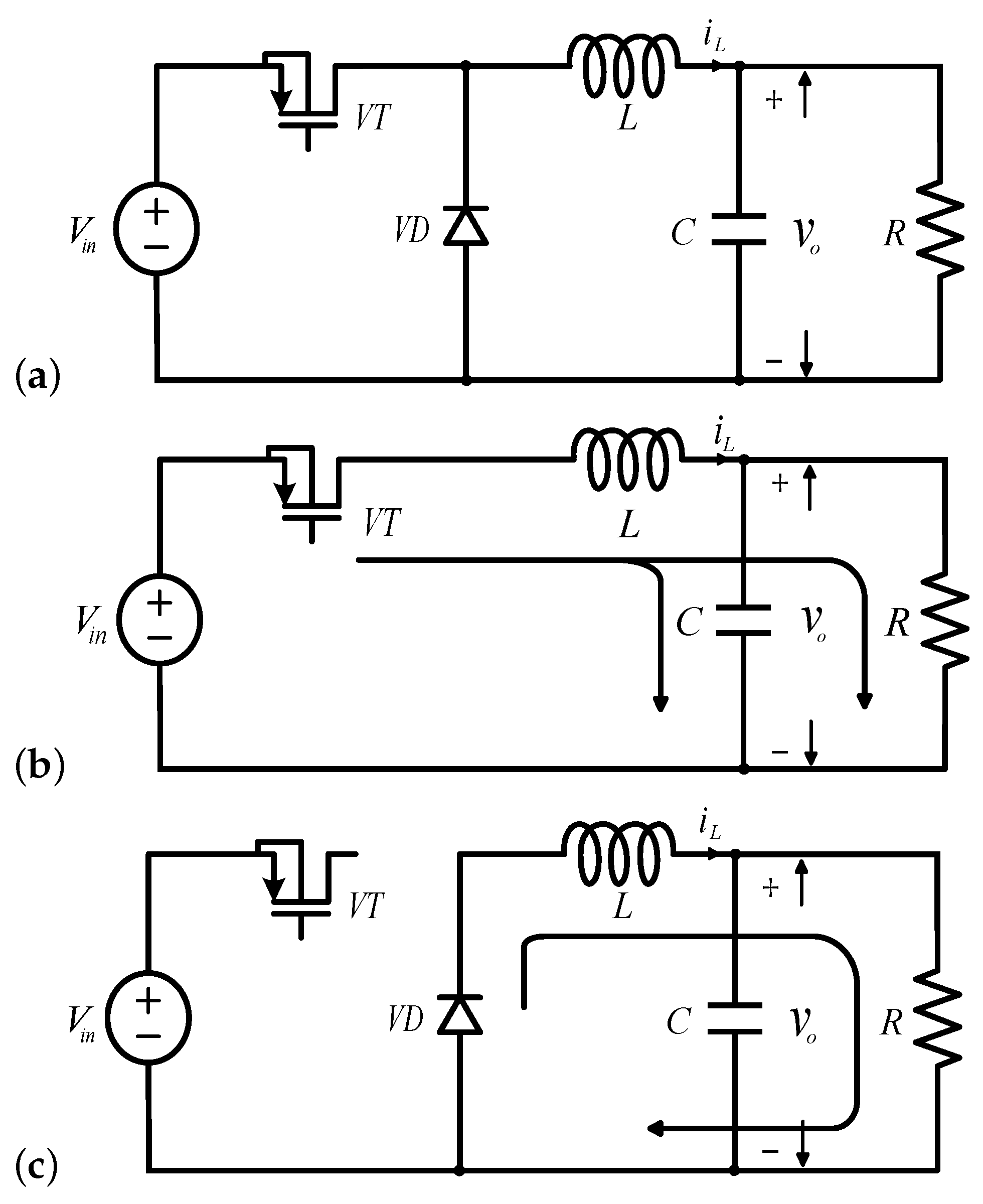
2.1. Modeling of DC-DC Buck Converter System

Generally, the DC-DC buck converter system consists of a switch tube, a rectifier diode, a low-pass filter network composed of inductance and capacitor, and a load resistance. The function of the switch tube is equivalent to a switch that is turned on and off under the control of the driving signal. A DC-DC buck converter circuit is shown in Figure 1, and the actual meanings of the parameters in the figure are as follows: DC voltage supply source $V_{in}$, PWM-driven switch device $VT$, diode $VD$, capacitor C, filter inductor L, and load resistance R.

Through the Kirchhoff voltage and current equation, the system model of on case and off case can be obtained, and the average model can be further obtained:

$$\left\{\begin{array}{c}{\dot{v}}_o=\frac{i_L}{C}-\frac{v_o}{RC},\hfill \\ {\dot{i}}_L=\frac{V_{in}\mu }{L}-\frac{v_o}{L},\hfill \end{array}\right.$$

(1)

where $v_o$ and $i_L$ are the values of the capacitor output voltage and inductor current, respectively. The duty ratio $\mu \in [0,1]$ represents a control signal that is compared with a triangular wave to generate a drive signal. As we all know, the converter system inevitably has uncertainties and disturbances. Taking these factors into full consideration, defining $x_1=v_0$ and $x_2=i_L$, the model in (1) can be presented in the following form: equation

$$\left\{\begin{array}{c}{\dot{x}}_1=-\frac{x_1}{C_0{R}_0}+\frac{x_2}{C_0}+d_1,\hfill \\ {\dot{x}}_2=-\frac{x_1}{L_0}+\frac{V_{in0}\mu }{L_0}+d_2.\hfill \end{array}\right.$$

(2)

where $C_0$, $R_0$, $L_0$, and $V_{i{n}_0}$ denote the nominal values of capacitance, resistance, inductance, and input voltage, respectively. The disturbances are expressed as $d_1=(\frac{1}{C}-\frac{1}{C_0})i_L+(\frac{1}{R_0{C}_0}-\frac{1}{RC})v_o$ and $d_2=(\frac{1}{L_0}-\frac{1}{L})v_o+(\frac{V_{in}}{L}-\frac{V_{i{n}_0}}{L_0})\mu$.

2.2. Analysis of Mathematical Model

The purpose of this section is to analyze the specific composition and source of disturbances $d_1$ and $d_2$ in system (2).

It is worth noting that disturbances and uncertainties are imposed on the DC-DC system through two different channels, thus affecting various performance indicators of the system. Here, the disturbance $d_2$ is on the same channel as the control input $\mu$, while the disturbance $d_1$ acts on the system through voltage and is on a different channel to the control input $\mu$, which is called a mismatched disturbance. When matched and mismatched disturbances exist at the same time, it is not a simple task to make the output voltage accurately track the desired trajectory, which also puts forward higher requirements for the design of observers and controllers.

2.3. Discretized Model

The following discretized model of the system (2) can be obtained as

$$\left\{\begin{array}{c}{x}_1\left(k\right)=x_1\left(k-1\right)+h\left[-\frac{1}{C_0{R}_0}{x}_1\left(k-1\right)+\frac{1}{C_0}{x}_2\left(k-1\right)+d_1\left(k-1\right)\right],\hfill \\ x_2\left(k\right)=x_2\left(k-1\right)+h\left[-\frac{1}{L_0}{x}_1\left(k-1\right)+\frac{V_{in0}}{L_0}\mu \left(k-1\right)+d_2\left(k-1\right)\right],\hfill \end{array}\right.$$

(3)

where h is the sampling period, and its value is $0.001$ s.

Combine system (3) and consider the following class of systems:

$$\left\{\begin{array}{c}{x}_k=F{x}_{k-1}+G_u{\mu }_{k-1}+G_d{d}_{k-1},\hfill \\ y_k=H{x}_k+v_k,\hfill \end{array}\right.$$

(4)

where $y_k$ is the measurement output and $v_k$ is the measurement noise,

$$F=\left[\begin{array}{cc}1-\frac{h}{C_0{R}_0}& \frac{h}{C_0}\\ -\frac{h}{L_0}& 1\end{array}\right],G_u=\left[\begin{array}{c}0\\ \frac{V_{in0}h}{L_0}\end{array}\right],G_d=\left[\begin{array}{cc}h& 0\\ 0& h\end{array}\right],H=\left[\begin{array}{cc}1& 0\\ 0& 1\end{array}\right].$$

(5)

To begin with, the following assumption is given:

Assumption 1.

$R_k$ is the measurement variance of noise, which can be obtained by the following equation:

$$E\left\{v_i{v}_j^T\right\}=\left\{\begin{array}{c}0,i\ne j,\hfill \\ R_k,i=j.\hfill \end{array}\right.$$

(6)

3. Design of the New Control Strategy (BSC + GPIO + KF) for DC-DC Buck Converter Systems

3.1. Proposed Disturbance Observer (GPIO + KF) Design

In order to improve the anti-disturbance performance of the system, a new observer is designed. The following is the design process of new method.

Assumption 2.

The n+1 derivative of $d_1$ tends to zero.

Assumption 3.

The n+1 derivative of $d_2$ tends to zero.

Assumption 4.

Covariance terms of ${\tilde{x}}_{k-1}^{+}$ and ${\tilde{d}}_{k-1}$ can be ignored.

Remark 1.

Because of the above assumptions, the Kalman filter gain becomes a suboptimal solution.

According to system (4), the prior estimation formula is as follows:

$${\widehat{x}}_k^{-}=F{\widehat{x}}_{k-1}^{+}+G_u{\mu }_{k-1}+G_d{\widehat{d}}_{k-1},$$

(7)

where ${\widehat{x}}_k^{-}$ is the prior estimation and ${\widehat{d}}_{k-1}$ is the disturbance estimation.

Similarly, the posterior estimation formula is as follows:

$${\widehat{x}}_k^{+}={\widehat{x}}_k^{-}+K_k\left(y_k-H{\widehat{x}}_k^{-}\right),$$

(8)

where ${\widehat{x}}_k^{+}$ is the posterior estimation and $K_k$ is the Kalman Filter gain.

Design of generalized proportional integral observer of $d_1$:

$$\left\{\begin{array}{c}{z}_1\left(k\right)=z_1\left(k-1\right)+h\left[-\frac{1}{C_0{R}_0}{z}_1\left(k-1\right)+\frac{1}{C_0}{\widehat{x}}_2^{+}\left(k-1\right)+z_2\left(k-1\right)\right]\hfill \\ +h{a}_1\left[{\widehat{x}}_1^{+}\left(k-1\right)-z_1\left(k-1\right)\right],\hfill \\ z_2\left(k\right)=z_2\left(k-1\right)+h{z}_3\left(k-1\right)+h{a}_2\left[{\widehat{x}}_1^{+}\left(k-1\right)-z_1\left(k-1\right)\right],\hfill \\ \dots ,\hfill \\ z_{n+1}\left(k\right)=z_{n+1}\left(k-1\right)+h{a}_{n+1}\left[{\widehat{x}}_1^{+}\left(k-1\right)-z_1\left(k-1\right)\right].\hfill \end{array}\right.$$

(9)

Design of generalized proportional integral observer of $d_2$:

$$\left\{\begin{array}{c}{\xi }_1\left(k\right)={\xi }_1\left(k-1\right)+h\left[-\frac{1}{L_0}{\widehat{x}}_1^{+}\left(k-1\right)+\frac{V_{in0}}{L_0}\mu \left(k-1\right)+{\xi }_2\left(k-1\right)\right]\hfill \\ +h{b}_1\left[{\widehat{x}}_2^{+}\left(k-1\right)-{\xi }_1\left(k-1\right)\right],\hfill \\ {\xi }_2\left(k\right)={\xi }_2\left(k-1\right)+h{\xi }_3\left(k-1\right)+h{b}_2\left[{\widehat{x}}_2^{+}\left(k-1\right)-{\xi }_1\left(k-1\right)\right],\hfill \\ \dots ,\hfill \\ {\xi }_{n+1}\left(k\right)={\xi }_{n+1}\left(k-1\right)+h{b}_{n+1}\left[{\widehat{x}}_2^{+}\left(k-1\right)-{\xi }_1\left(k-1\right)\right].\hfill \end{array}\right.$$

(10)

The following contents will introduce solution of the Kalman Filter gain.

The prior estimation error is solved as follows:

$$\begin{array}{c}{x}_k-{\widehat{x}}_k^{-}=F{x}_{k-1}+G_u{\mu }_{k-1}+G_d{d}_{k-1}-F{\widehat{x}}_{k-1}^{+}-G_u{\mu }_{k-1}-G_d{\widehat{d}}_{k-1}\hfill \\ =F\left(x_{k-1}-{\widehat{x}}_{k-1}^{+}\right)+G_d\left(d_{k-1}-{\widehat{d}}_{k-1}\right).\hfill \end{array}$$

(11)

After calculating the prior estimation error, calculate the covariance matrix of the prior estimation:

$$\begin{array}{c}{P}_k^{-}=E\left\{\left(x_k-{\widehat{x}}_k^{-}\right){\left(x_k-{\widehat{x}}_k^{-}\right)}^T\right\}\hfill \\ =E\left\{F{\tilde{x}}_{k-1}^{+}\tilde{x}{{}_{k-1}^{+}}^T{F}^T\right\}-E\left\{F{\tilde{x}}_{k-1}^{+}{\tilde{d}}_{k-1}^T{G}_d^T\right\}-E\left\{G_d{\tilde{d}}_{k-1}\tilde{x}{{}_{k-1}^{+}}^T{F}^T\right\}+E\left\{G_d{\tilde{d}}_{k-1}{\tilde{d}}_{k-1}^T{G}_d^T\right\}\hfill \\ =E\left\{F{\tilde{x}}_{k-1}^{+}\tilde{x}{{}_{k-1}^{+}}^T{F}^T\right\}+E\left\{G_d{\tilde{d}}_{k-1}{\tilde{d}}_{k-1}^T{G}_d^T\right\}\hfill \\ =F{P}_{k-1}^{+}{F}^T+G_d{Q}_d{G}_d^T,\hfill \end{array}$$

(12)

where $Q_d$ is the disturbance estimation error covariance. Obviously, we can obtain the following initial values:

$$P_0^{-}=E\left\{{\tilde{x}}_0^{-}\tilde{x}{{}_0^{-}}^T\right\}.$$

(13)

The posteriori estimation error is solved as follows:

$$\begin{array}{c}{x}_k-{\widehat{x}}_k^{+}=x_k-{\widehat{x}}_k^{-}-K_k\left(H{x}_k+v_k-H{\widehat{x}}_k^{-}\right)\hfill \\ =\left(I-K_{k}H\right)\left(x_k-{\widehat{x}}_k^{-}\right)-K_k{v}_k.\hfill \end{array}$$

(14)

After calculating the posteriori estimation error, calculate the covariance matrix of the posteriori estimation:

$$\begin{array}{c}{P}_k^{+}=E\left\{\left(x_k-{\widehat{x}}_k^{+}\right){\left(x_k-{\widehat{x}}_k^{+}\right)}^T\right\}\hfill \\ =E\left\{\left(I-K_{k}H\right){\tilde{x}}_k^{-}\tilde{x}{{}_k^{-}}^T{\left(I-K_{k}H\right)}^T\right\}+E\left\{\left(I-K_{k}H\right){\tilde{x}}_k^{-}{v}_k^T{K}_k^T\right\}\hfill \\ +E\left\{K_k{v}_k\tilde{x}{{}_k^{-}}^T{\left(I-K_{k}H\right)}^T\right\}+E\left\{K_k{v}_k{v}_k^T{K}_k^T\right\}\hfill \\ =\left(I-K_{k}H\right)P_k^{-}{\left(I-K_{k}H\right)}^T+K_k{R}_k{K}_k^T.\hfill \end{array}$$

(15)

In order to determine the gain $K_k$, we minimize the trace of $P_k^{+}$, which is equivalent to minimizing the length of the estimation error vector:

$$J\left(K_k\right)=Tr\left(P_k^{+}\right).$$

(16)

The necessary condition of minimizing $J\left(K_k\right)$ is

$$\frac{\partial J}{\partial K_k}=-2\left(I-K_{k}H\right)P_k^{-}{H}^T+2K_k{R}_k=0$$

(17)

Solving (17) for $K_k$ gives:

$$K_k=P_k^{-}{H}^T{\left(H{P}_k^{-}{H}^T+R_k\right)}^{-1}.$$

(18)

Then, substituting (18) into (15), one obtains

$$\begin{array}{c}{P}_k^{+}=P_k^{-}-K_{k}H{P}_k^{-}-P_k^{-}{H}^T{K}_k^T+K_k\left[H{P}_k^{-}{H}^T+R_k\right]K_k^T\hfill \\ =P_k^{-}-K_{k}H{P}_k^{-}.\hfill \end{array}$$

(19)

3.2. Stability Analysis of the Proposed Disturbance Observer

Definition 1

([26]). Consider a discrete-time nonlinear system (20) of the general form:

$$x\left(k+1\right)=f\left(x\left(k\right),u\left(k\right)\right),$$

(20)

where states $x\left(k\right)$ are in $R^n$, and control values $u\left(k\right)$ in $R^m$, for some n and m, and for each time instant $k\in Z_{+}$. Assume that $f:R^n\times R^m\to R^n$ is continuous and $f\left(0,0\right)=0$. System (26) is (globally) input-to-state stable (ISS) if a $KL$ function $\beta :R_{\ge 0}\times R_{\ge 0}\to R_{\ge 0}$ and a K function γ exist such that, for each input $u\in l_{\infty }^m$ and each $\zeta \in R^n$, for every $k\in Z_{+}\backslash \left\{0\right\}$, it holds that:

$$\left|x\left(k,\zeta ,u\right)\right|\le \beta \left(\left|\zeta \right|,k\right)+\gamma \left(∥u_{\left[k-1\right]}∥\right),$$

(21)

where term $u_{\left[k-1\right]}$ denotes the truncation of u at $k-1$.

Definition 2.

A continuous function $V:R^n\to R_{\ge 0}$ is called an ISS-Lyapunov function for system (1) if the following holds:

(1)

$K_{\infty }$ function ${\alpha }_1$, ${\alpha }_2$ exists such that

$${\alpha }_1\left(\left|\zeta \right|\right)\le V\left(\zeta \right)\le {\alpha }_2\left(\left|\zeta \right|\right),\forall \zeta \in R^n.$$

(22)

(2)

$K_{\infty }$ function ${\alpha }_3$ and a K function σ, for all $\zeta \in R^n$, and for all $u\in R^m$ exist such that:

$$V\left(f\left(\zeta ,u\right)\right)-V\left(\zeta \right)\le -{\alpha }_3\left(\left|\zeta \right|\right)+\sigma \left(\left|u\right|\right).$$

(23)

Lemma 1

([26]). If system (20) admits an ISS-Lyapunov function, then it is ISS.

Theorem 1.

On the basis of the steady-state Kalman filter gain, and when $A_o$ is a Schur matrix, then we can find an ISS Lyapunov function V. According to Lemma 1, the observer is ISS.

Proof of Theorem 1.

The state estimation errors of the DC-DC converter system are defined as

$$e_o\left(k-1\right)=\left[\begin{array}{c}{e}_1\left(k-1\right)\\ e_{x_1}\left(k-1\right)\\ e_{d_1}\left(k-1\right)\\ ⋮\\ e_{d_1^{\left(n-1\right)}}\left(k-1\right)\\ e_2\left(k-1\right)\\ e_{x_2}\left(k-1\right)\\ e_{d_2}\left(k-1\right)\\ ⋮\\ e_{d_2^{\left(n-1\right)}}\left(k-1\right)\end{array}\right]=\left[\begin{array}{c}{x}_1\left(k-1\right)-{\widehat{x}}_1^{+}\left(k-1\right)\\ x_1\left(k-1\right)-z_1\left(k-1\right)\\ d_1\left(k-1\right)-z_2\left(k-1\right)\\ ⋮\\ d_1^{\left(n-1\right)}\left(k-1\right)-z_n\left(k-1\right)\\ x_2\left(k-1\right)-{\widehat{x}}_2^{+}\left(k-1\right)\\ x_2\left(k-1\right)-{\xi }_1\left(k-1\right)\\ d_2\left(k-1\right)-{\xi }_2\left(k-1\right)\\ ⋮\\ d_2^{\left(n-1\right)}\left(k-1\right)-{\xi }_n\left(k-1\right)\end{array}\right].$$

(24)

The observer error dynamics can be expressed as

$$e_o\left(k\right)=A_o{e}_o\left(k-1\right)+\dot{d}\left(k-1\right).$$

(25)

We can obtain the relevant parameters in the above formula:

$$\dot{d}\left(k-1\right)={\left[\begin{array}{cccccccccc}{D}_1& 0& 0& \cdots & d_1^{\left(n\right)}\left(k-1\right)& D_2& 0& 0& \cdots & d_2^{\left(n\right)}\left(k-1\right)\end{array}\right]}^T,$$

(26)

where $D_1=-K_{{11}_s}{v}_1\left(k-1\right)-K_{{12}_s}{v}_2\left(k-1\right)$ and $D_2=-K_{{21}_s}{v}_1\left(k-1\right)-K_{{22}_s}{v}_2\left(k-1\right)$.

$$A_o=\left[\begin{array}{cccccccccc}{B}_1& 0& B_2& \cdots & 0& B_3& 0& -h{K}_{{12}_s}& \cdots & 0\\ h{a}_1& B_4& h& \cdots & 0& \frac{h}{C}& 0& 0& \cdots & 0\\ h{a}_2& -h{a}_2& 1& \ddots & 0& 0& 0& 0& \ddots & 0\\ ⋮& ⋮& ⋮& \ddots & ⋮& ⋮& ⋮& ⋮& \ddots & 0\\ h{a}_{n+1}& -h{a}_{n+1}& 0& \cdots & 1& 0& 0& 0& \cdots & 0\\ B_5& 0& -h{K}_{{21}_s}& \cdots & 0& B_6& 0& B_7& \cdots & 0\\ -\frac{h}{L_0}& 0& 0& \cdots & 0& h{b}_1& 1-h{b}_1& h& \cdots & 0\\ 0& 0& 0& \ddots & 0& h{b}_2& -h{b}_2& 1& \ddots & 0\\ ⋮& ⋮& ⋮& \ddots & ⋮& ⋮& ⋮& ⋮& \ddots & ⋮\\ 0& 0& 0& \cdots & 0& h{b}_{n+1}& -h{b}_{n+1}& 0& \cdots & 1\end{array}\right],$$

(27)

where, $B_1=\left(1-K_{{11}_s}\right)\left(1-\frac{h}{R_0{C}_0}\right)+\frac{h{K}_{{12}_s}}{L}$, $B_2=h\left(1-K_{{11}_s}\right)$, $B_3=\left(1-K_{{11}_s}\right)\frac{h}{C_0}-K_{{12}_s}$, $B_4=1-\frac{h}{R_0{C}_0}-h{a}_1$, $B_5=-K_{{21}_s}\left(1-\frac{h}{R_0{C}_0}\right)-\frac{h}{L}\left(1-K_{{22}_s}\right)$, $B_6=-\frac{h{K}_{{21}_s}}{C_0}+\left(1-K_{{22}_s}\right)$, and $B_7=h\left(1-K_{{22}_s}\right)$.

The gains of the generalized proportional integral observer are appropriately selected by pole placement so that $A_0$ is a Schur matrix. According to Lemma 1, the observer is ISS. This completes the proof. □

3.3. Composite Controller Design and Analysis

The objective of the controller is to make the output voltage track the reference voltage. When the general framework of backstepping control is applied to the design, a two-step design is adopted because the inverter system is a second-order system. In addition, the reference voltage is constant in the system, so its first derivative and second derivative need not be considered in the two-step design.

Theorem 2.

Under Assumptions 2 and 3, if the controller is designed for the buck converter (2) as

$$\mu =\frac{L_0{C}_0}{V_{in0}}\left\{\frac{1}{L_0{C}_0}{x}_1-\frac{1}{C_0}{\widehat{d}}_2+\left(\frac{1}{C_0{R}_0}+k_1-k_2\right)z_2-\left[\left(\frac{1}{C_0{R}_0}+k_1\right)k_1+k_3\right]z_1\left.+{\dot{\widehat{d}}}_1\right\}\right.$$

(28)

where the controller gains $k_1$ and $k_2$ are properly selected such that A in (34) is Hurwitz matrix, then the output voltage $v_0$ tracks the reference voltage $v_r$.

Proof of Theorem 2.

The proof includes two steps.

Step 1: Denote $z_1=x_1-x_{1ref}$, and differentiate $z_1$ with respect to time along (2), which implies:

$${\dot{z}}_1=-\frac{1}{C_0{R}_0}{z}_1+\frac{1}{C_0}{x}_2+d_1.$$

(29)

The virtual control law can be shown as follows:

$$x_2^{*}=C_0\left(\frac{1}{C_0{R}_0}{z}_1-k_1{z}_1-{\widehat{d}}_1\right).$$

(30)

Step 2: Denote $z_2=\frac{1}{C_0}\left(x_2-x_2^{*}\right)$. So, ${\dot{z}}_1$ can be rewritten as follows:

$${\dot{z}}_1=-\frac{1}{C_0{R}_0}{z}_1+\left(z_2+\frac{1}{C_0}{x}_2^{*}\right)+d_1=z_2-k_1{z}_1+e_{d_1},$$

(31)

where ${e_d}_1=d_1-{\widehat{d}}_1$.

Differentiating $z_2$ with respect to time along (2), we have

$${\dot{z}}_2=-\frac{1}{L_0{C}_0}{x}_1+\frac{V_{in0}}{L_0{C}_0}\mu +\frac{1}{C_0}{d}_2-\left(\frac{1}{C_0{R}_0}+k_1\right)\left(z_2-k_1{z}_1+e_{d_1}\right)-{\dot{\widehat{d}}}_1.$$

(32)

The control law is designed as (28). Combining (28) and (31), we can obtain:

$$\begin{array}{cc}\hfill {\dot{z}}_2& =\left\{\frac{1}{L_0{C}_0}{x}_1-\frac{1}{C_0}{\widehat{d}}_2+\left(\frac{1}{C_0{R}_0}+k_1-k_2\right)z_2-\left[\left(\frac{1}{C_0{R}_0}+k_1\right)k_1+k_3\right]z_1\left.+{\dot{\widehat{d}}}_1\right\}\right.\hfill \\ & -\frac{1}{L_0{C}_0}{x}_1+\frac{1}{C_0}{d}_2-\left(\frac{1}{C_0{R}_0}+k_1\right)\left(z_2-k_1{z}_1+e_{d_1}\right)-{\dot{\widehat{d}}}_1.\hfill \end{array}$$

(33)

$${\dot{z}}_2=-z_1-k_2{z}_2-\left(\frac{1}{C_0{R}_0}+k_1\right)e_{d_1}+\frac{1}{C_0}{e}_{d_2},$$

(34)

where $e_{d_2}=d_2-{\widehat{d}}_2$.

Ulteriorly, the system can be expressed as

$$\left\{\begin{array}{c}{\dot{z}}_1=z_2-k_1{z}_1+e_{d_1}\hfill \\ {\dot{z}}_2=-z_1-k_2{z}_2+\frac{1}{C_0}{e}_{d_2}-\left(\frac{1}{C_0{R}_0}+k_1\right)e_{d_1}\hfill \end{array}\right.$$

(35)

The system can be rewritten as follows:

$$\dot{z}=Az+B{e}_d,$$

(36)

where $A=\left[\begin{array}{cc}-k_1& 1\\ -1& -k_2\end{array}\right]$ and $B=\left[\begin{array}{cc}1& 0\\ -\left(\frac{1}{C_0{R}_0}+k_1\right)& \frac{1}{C_0}\end{array}\right]$.

Select the proper parameters to make A a Hurwitz matrix, the system $\dot{z}=Az$ is globally uniformly asymptotically stable. Based on this, it is easy to verity that system (36) is ISS with the input $e_d$. According to Theorem 1, $\underset{t\to \infty }{lim}{e}_d=0$, it follows from Lemma 1 that $\underset{t\to \infty }{lim}z=0$.

This completes the proof. □

Remark 2.

Take the form of the reference signal again and emphasize that the first and second derivatives of the reference signal have no influence on the controller design and stability analysis.

4. Experimental Tests

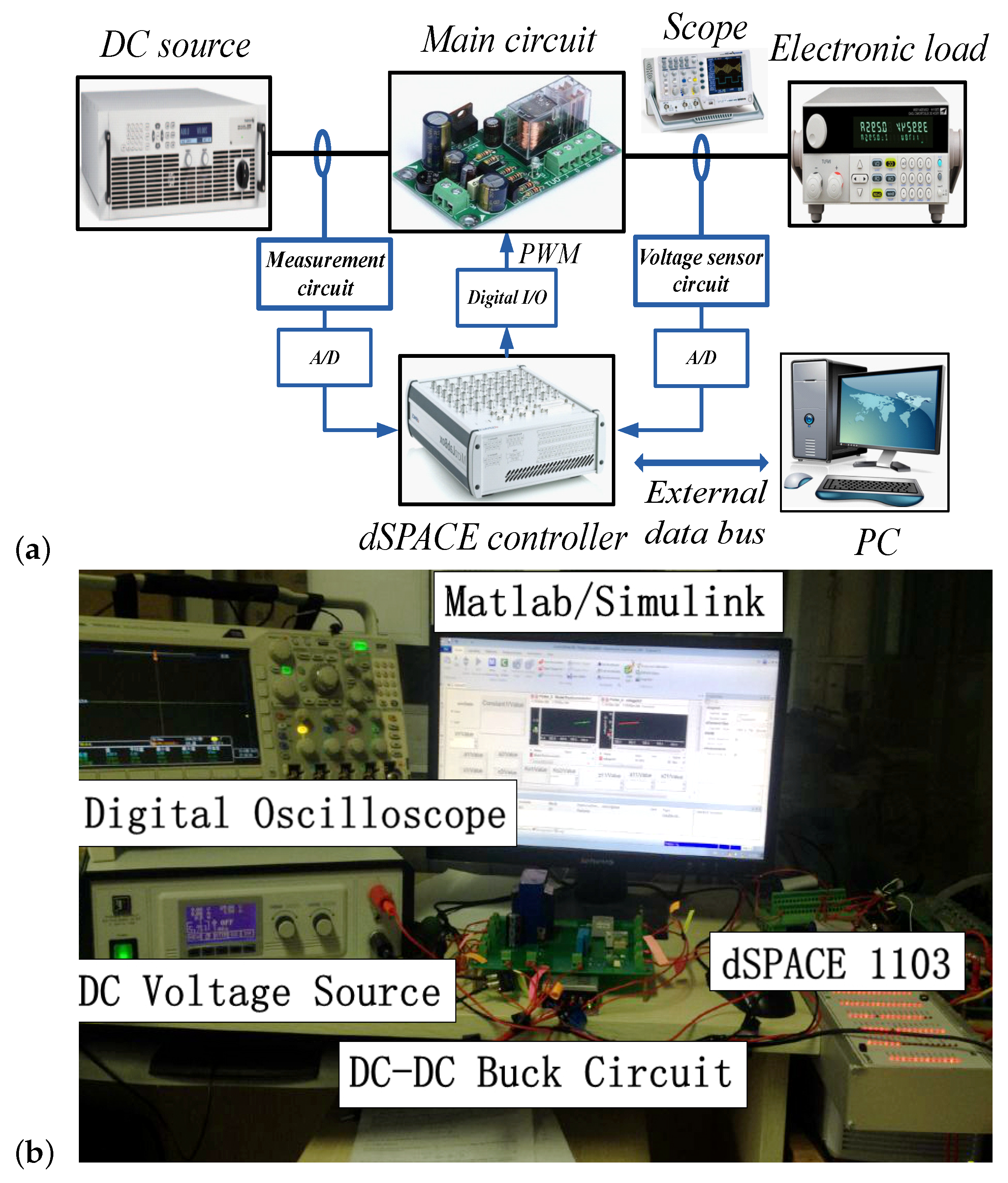
4.1. Experimental Tests Setup

In order to verify the effectiveness of the proposed control method, the experiment was carried out on a self-developed experiment platform. The experiment platform is mainly composed of computer (Host PC), integrated controller (dSPACE1103), a DC-DC buck converter, a DC power supply, a digital oscilloscope, voltage, and current sensors, as shown in Figure 2. The sampling period is $0.001$ s. The measured output voltage is converted by the 16 bit A/D converter of the real-time controller. The output waveforms are recorded by digital oscilloscope and dSPACE 1103.

The reference voltage of the buck converter is 9 V (constant signal). The structural parameters of the DC-DC buck converter are shown in

Table 1. Parameter values of the buck converter circuit.

Description	Parameters	Nominal Values
Input voltage	$V_{i{n}_0}$	20 V
Reference voltage	$v_r$	9 V
Inductance	$L_0$	$1\times {10}^{-2}$ H
Capacitance	$C_0$	$7\times {10}^{-5}$ F
Load resistance	$R_0$	$30\Omega$

.

The controller parameters of BSC and GPIO, ESO + KF, and GPIO + KF are selected and shown in

Table 2. Control parameters for DC–DC buck converter.

Controllers	Observers	Experimental Parameters
BSC	GPIO	$k_1=150$, $k_2=550$, $p=-200$
BSC	ESO + KF	$k_1=150$, $k_2=550$, $p=-300$
BSC	GPIO + KF	$k_1=150$, $k_2=550$, $p=-500$

:

The selection criteria of KF parameters $P_0$, $R_k$, and $Q_d$ and the calculation process of the Kalman gain are consistent with the methods in [25] and will not be repeated here.

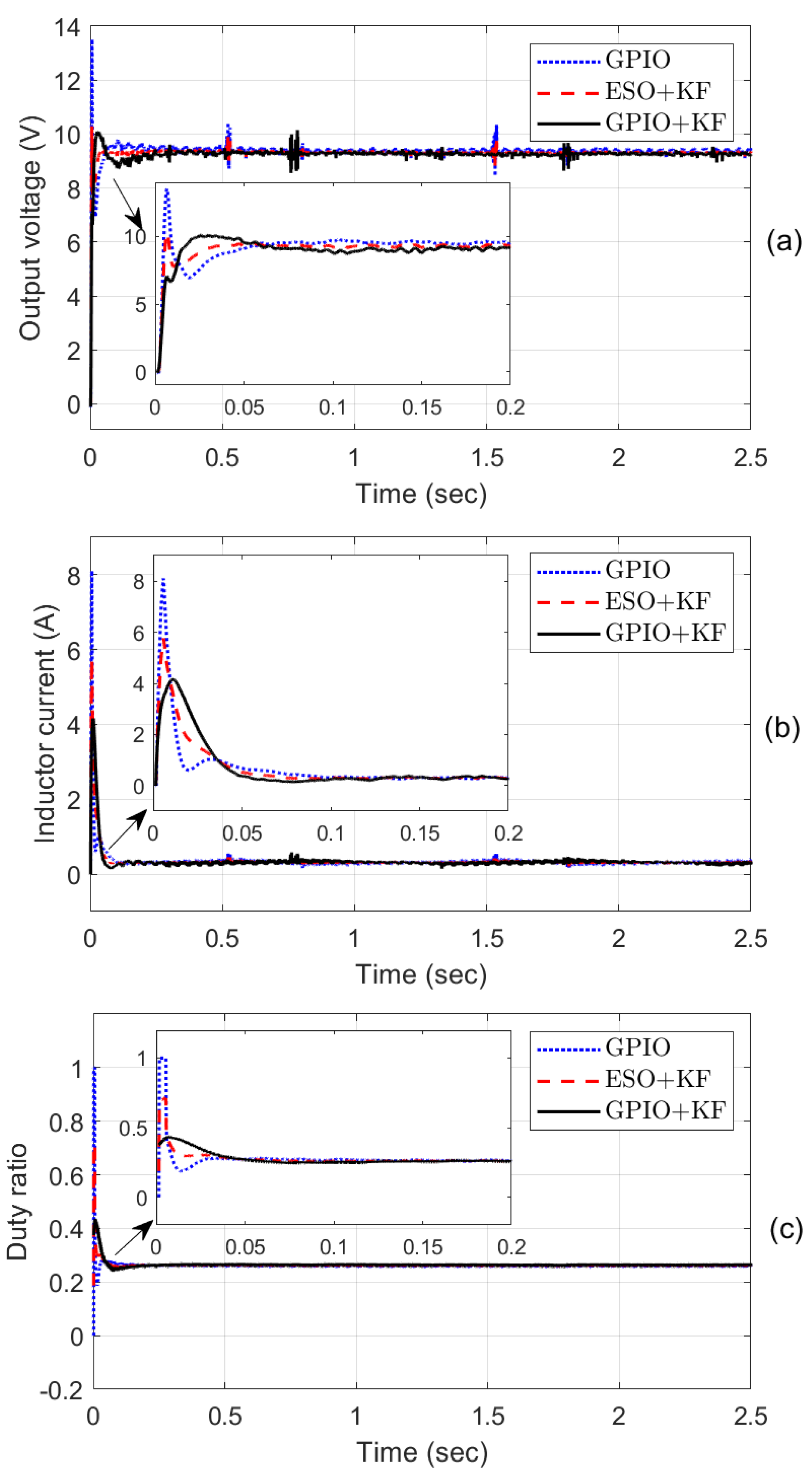
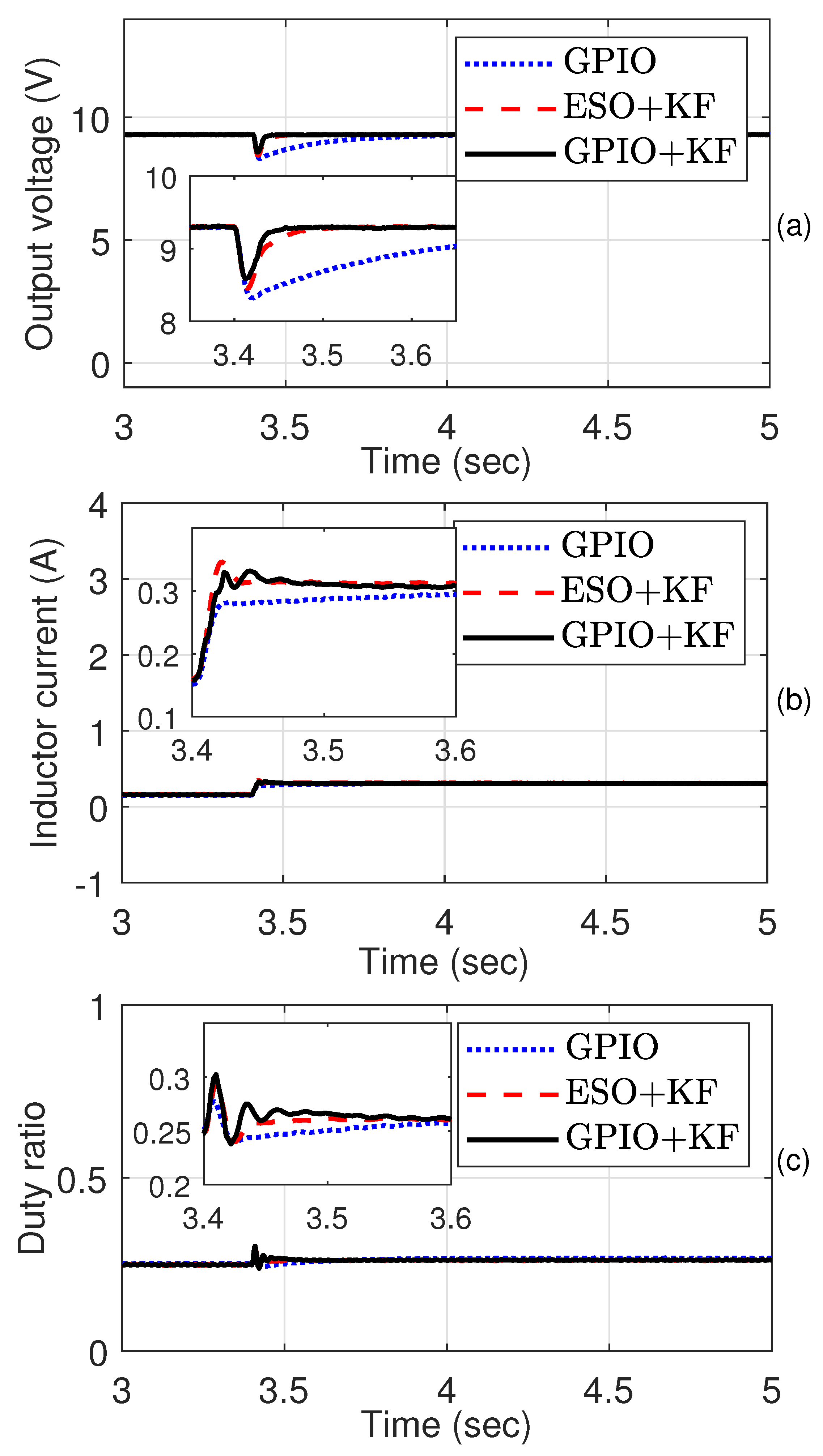
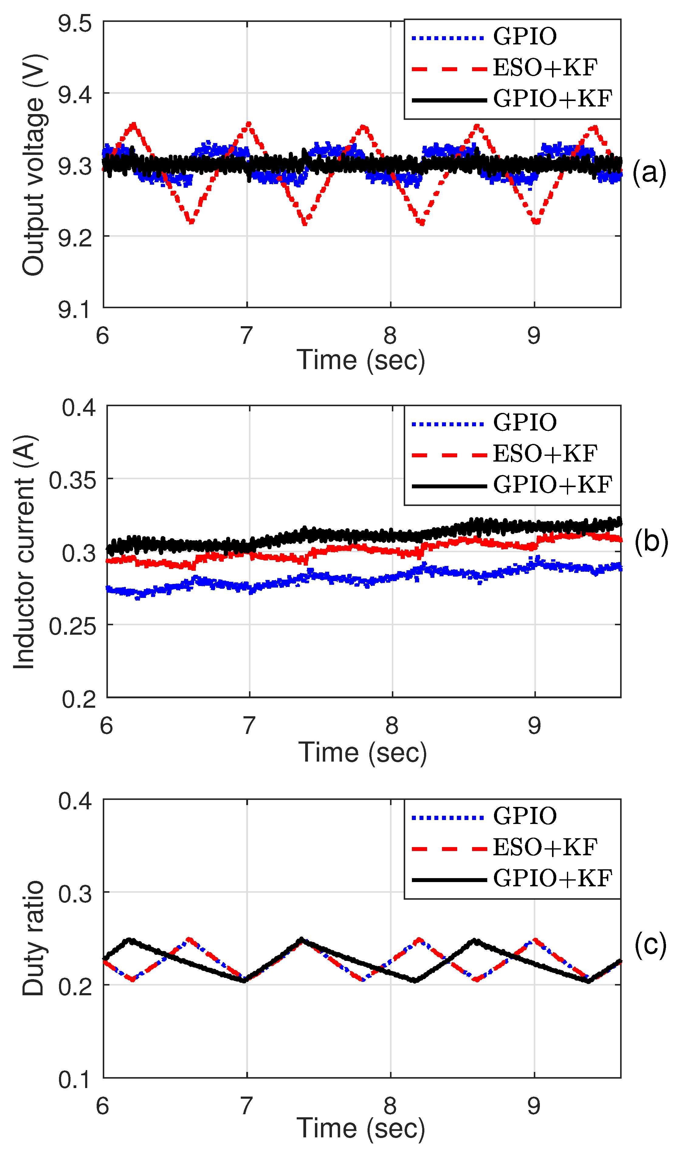
4.2. Experiment Results

Case I. The system is just started:

Figure 3a–c are the waveform curves of the output voltage, inductor current, and duty ratio, respectively, when the system is just started. As shown in Figure 3a, in all three control schemes, the output voltage can track the reference voltage, and the effect is good. At the same time, the three schemes have some overshoot, especially when the observer only uses GPIO. In Figure 3b,c, when the system is just started, the inductor current-response curves and duty-ratio curves of the three control schemes are similar.

Case II. Disturbance is form of step:

At $t=3.4$ s, the sudden change of input voltage is taken as the step disturbance of the system. Specifically, the input voltage is expected to change from its nominal value. Figure 4a–c are the waveform curves of output voltage, inductor current, and duty ratio, respectively, when disturbance is the form of step. As shown in Figure 4a, the proposed method has stronger anti-disturbance ability, but other methods have the same effect on such disturbance, so it can only be said that it has a small advantage. In Figure 4b,c, when disturbance is the form of step, the inductor current response curves and duty ratio curves of the three control schemes are almost the same.

Case III. Disturbance is the polynomial form of time series:

At $t=6$ s, a sawtooth disturbance is added to the nominal value of the input voltage as a polynomial disturbance of the time series. Figure 5a–c are the waveform curves of the output voltage, inductor current, and duty ratio, respectively, when disturbance is is the polynomial form of time series. As shown in Figure 5a,b, it is not difficult to find that the advantages of the proposed method are particularly obvious. Two other controllers cannot remove the effects caused by such disturbance. In general, ESO can only suppress a slowly varying disturbance. Even if the Kalman filter structure is added, it can only reduce its sensitivity to noise, and it cannot adequately observe and compensate for polynomial disturbance. However, GPIO can suppress polynomial disturbance in essence. Even without the Kalman filter structure, GPIO is less sensitive to noise, but it is effective to disturbance itself. Therefore, GPIO is better than ESO + KF.

5. Conclusions

A new control strategy is designed for the DC-DC buck converter system with uncertainties, disturbances, and noise at the same time. This strategy uses the composite form of the Kalman filter and generalized proportional integral observer to estimate the disturbances, which makes a tradeoff between the speed/accuracy of the GPIO to observe states and disturbances and its sensitivity to noise. This strategy introduces disturbance estimation into the design of the virtual control law of the backstepping controk, which further improves the tracking performance and anti-disturbance ability. The theoretical design of the strategy has undergone strict stability analysis, and hardware experiments have also verified its feasibility and effectiveness.

References

1. Ding, S.; Liu, L.; Zheng, W. Sliding mode direct yaw-moment control design for in-wheel electric vehicles. IEEE Trans. Ind. Electron. 2017, 64, 6752–6762. [Google Scholar] [CrossRef]
2. Sun, B.; Gao, Z. A DSP-based active disturbance rejection control design for a 1-kW H-bridge DC-DC power converter. IEEE Trans. Ind. Electron. 2005, 53, 1271–1277. [Google Scholar] [CrossRef] [Green Version]
3. Wang, Z.; Li, S.; Yang, J.; Li, Q. Current sensorless sliding mode control for direct current–alternating current inverter with load variations via a usdo approach. IET Power Electron. 2018, 11, 1389–1398. [Google Scholar] [CrossRef]
4. Guo, T.; Wang, Z.; Wang, X.; Li, S.; Li, Q. A simple control approach for buck converters with current-constrained technique. IEEE Trans. Control. Syst. Technol. 2017, 27, 418–425. [Google Scholar] [CrossRef]
5. Wang, Z.; Li, S.; Wang, J.; Li, Q. Generalized proportional integral observer based backstepping control for DC-DC buck converters with mismatched disturbances. In Proceedings of the IEEE International Conference on Industrial Technology (ICIT), Tehran, Iran, 25–26 January 2016. [Google Scholar]
6. Alvarez-Ramirez, J.; Espinosa-Perez, G.; Noriega-Pineda, D. Currentmode control of DC-DC power converters: A backstepping approach. Int. J. Robust Nonlinear Control. 2003, 13, 421–442. [Google Scholar] [CrossRef]
7. Wang, J.; Li, S.; Yang, J.; Wu, B.; Li, Q. Extended state observer-based sliding mode control for PWM-based DC-DC buck power converter systems with mismatched disturbances. IET Contr. Theory Appl. 2015, 9, 579–586. [Google Scholar] [CrossRef]
8. Hamed, S.; Hamed, M.; Sbita, L. Robust voltage control of a buck DC-DC converter: A sliding mode approach. Energies 2022, 15, 6128. [Google Scholar] [CrossRef]
9. Mobayen, S.; Bayat, F.; Lai, C. Adaptive global sliding mode controller design for perturbed DC-DC buck converters. Energies 2021, 14, 1249. [Google Scholar] [CrossRef]
10. Zhang, C.; Wang, J.; Li, S.; Wu, B.; Qian, C. Robust control for PWM-based DC-DC buck power converters with uncertainty via sampled-data output feedback. IEEE Trans. Power Electron. 2015, 30, 504–515. [Google Scholar] [CrossRef]
11. Lin, P.; Zhang, C.; Wang, P.; Xiao, J. A decentralized composite controller for unified voltage control with global system large-signal stability in DC microgrids. IEEE Trans. Smart Grid 2019, 10, 5075–5091. [Google Scholar] [CrossRef]
12. Yang, Y.; Tan, S.; Hui, S. Adaptive reference model predictive control with improved performance for voltage-source inverters. IEEE Trans. Control Syst. Technol. 2018, 26, 724–731. [Google Scholar] [CrossRef]
13. Yang, J.; Wu, B.; Li, S.; Yu, X. Design and qualitative robustness analysis of an dobc approach for dc-dc buck converters with unmatched circuit parameter perturbations. IEEE Trans. Circuits Syst. I-Regul. Pap. 2016, 63, 551–560. [Google Scholar] [CrossRef]
14. Choi, K.; Dong, S.; Kim, S. Disturbance observer-based offset-free global tracking control for input-constrained LTI systems with DC/DC buck converter applications. Energies 2020, 13, 4079. [Google Scholar] [CrossRef]
15. Ghosh, R.; Narayanan, G. Generalized feedforward control of singlephase PWM rectifiers using disturbance observers. IEEE Trans. Ind. Electron. 2007, 54, 984–993. [Google Scholar] [CrossRef] [Green Version]
16. Lakomy, K.; Madonski, R.; Dai, B. Active disturbance rejection control design with suppression of sensor noise effects in application to DC–DC buck power converter. IEEE Trans. Ind. Electron. 2022, 69, 819–824. [Google Scholar] [CrossRef]
17. Han, J. From PID to active disturbance rejection control. IEEE Trans. Ind. Electron. 2009, 56, 900–906. [Google Scholar] [CrossRef]
18. Lu, J.; Savaghebi, M.; Ghias, A. A reduced-order generalized proportional integral observer-based resonant super-twisting sliding mode control for grid-connected power converters. IEEE Trans. Ind. Electron. 2021, 68, 5897–5908. [Google Scholar] [CrossRef]
19. Sira-Ramirez, C.; Nunez, A.; Visairo, N. Robust sigma-delta generalised proportional integral observer based control of a buck converter with uncertain loads. Int. J. Control 2010, 83, 1631–1640. [Google Scholar] [CrossRef]
20. Gao, Z. Scaling and bandwidth-parameterization based controller tuning. In Proceedings of the American Control Conference (ACC), Denver, CO, USA, 4–6 June 2003. [Google Scholar]
21. Prasov, A.; Khalil, H. A nonlinear high-gain observer for systems with measurement noise in a feedback control framework. IEEE Trans. Autom. Control. 2013, 58, 569–580. [Google Scholar] [CrossRef]
22. Pu, Z.; Yuan, R.; Yi, J.; Tan, X. A class of adaptive extended state observers for nonlinear disturbed systems. IEEE Trans. Ind. Electron. 2015, 62, 5858–5869. [Google Scholar] [CrossRef]
23. Bai, W.; Xue, W.; Huang, Y.; Fang, H. On extended state based kalman filter design for a class of nonlinear time-varying uncertain systems. Sci. China Inf. Sci. 2018, 61, 042201-1–042201-16. [Google Scholar] [CrossRef]
24. Xue, W.; Bai, W.; Yang, S.; Song, K.; Huang, Y.; Xie, H. ADRC with adaptive extended state observer and its application to air-fuel ratio control in gasoline engines. IEEE Trans. Ind. Electron. 2015, 62, 5847–5857. [Google Scholar] [CrossRef]
25. Sun, H.; Madonski, R.; Li, S.; Zhang, Y.; Xue, W. Composite control design for systems with uncertainties and noise using combined extended state observer and kalman filter. IEEE Trans. Ind. Electron. 2022, 69, 4119–4228. [Google Scholar] [CrossRef]
26. Jiang, Z.; Wang, Y. Input-to-state stability for discrete-time nonlinear systems. Automatica 2001, 37, 857–869. [Google Scholar] [CrossRef]
Figure 1. Circuit diagram of buck converter. (a) An average case. (b) A switch ON case. (c) A switch OFF case.
Actuators 12 00020 g001
Figure 2. Experimental test setup. (a) Configuration. (b) Photograph of Hardware.
Actuators 12 00020 g002
Figure 3. Waveform curves when the system is just started. (a) Output voltage. (b) Inductor current. (c) Duty ratio.
Actuators 12 00020 g003
Figure 4. Waveform curves when disturbance is form of step. (a) Output voltage. (b) Inductor current. (c) Duty ratio.
Actuators 12 00020 g004
Figure 5. Waveform curves when disturbance is polynomial form of time series. (a) Output voltage. (b) Inductor current. (c) Duty ratio.
Actuators 12 00020 g005