Real-Time Modeling of Vehicle’s Longitudinal-Vertical Dynamics in ADAS Applications

Abstract

The selection of an appropriate method for modeling vehicle dynamics heavily depends on the application. Due to the absence of human intervention, the demand for an accurate and real-time model of vehicle dynamics for intelligent control increases for autonomous vehicles. This paper develops a multibody vehicle model for longitudinal-vertical dynamics applicable to advanced driver assistance (ADAS) applications. The dynamic properties of the chassis, suspension, and tires are considered and modeled, which results in accurate vehicle dynamics and states. Unlike the vehicle dynamics models built into commercial software packages, such as ADAMS and CarSim, the proposed nonlinear dynamics model poses the equations of motion using a subset of relative coordinates. Therefore, the real-time simulation is conducted to improve riding performance and transportation safety. First, a vehicle system is modeled using a semi-recursive multibody dynamics formulation, and the vehicle kinematics and dynamics are accurately calculated using the system tree-topology. Second, a fork-arm removal technique based on the rod-removal technique is proposed to reduce the number of bodies, relative coordinates, and equations constrained by loop-closure. This increase the computational efficiency even further. Third, the dynamic simulations of the vehicle are performed on bumpy and sloping roads. The accuracy and efficiency of the numerical results are compared to the reference data. The comparative results demonstrate that the proposed vehicle model is effective. This efficient model can be utilized for the intelligent control of vehicle ADAS applications, such as forward collision avoidance, adaptive cruise control, and platooning.

1. Introduction

In recent years, automated driving has been an active research topic. Several advanced driver assistance systems (ADAS) have been studied in terms of ride comfort, handling performance, transportation safety, and efficiency [1,2]. This includes several essential technologies, such as electronic stability control [3], active front steering control [4], autonomous emergency braking [5], forward collision avoidance [6], adaptive cruise control [7], and platooning [8]. These ADAS applications necessitate efficient vehicle models, either for longitudinal, lateral, or vertical dynamics, or for coupling these types due to intelligent control [9,10].

In the near future, it is expected that highly autonomous vehicles that operate without human intervention will be on the road, significantly enhancing transportation safety and efficiency. Acquiring vehicle states and dynamic responses requires precise models to achieve these objectives [11]. Simplified vehicle models that describe the longitudinal, lateral, and vertical dynamics separately are insufficient for vehicle coupling dynamics. In complex driving conditions, coupling dynamics models, such as longitudinal–lateral or longitudinal-vertical models, is crucial [12,13]. By analyzing and controlling the coupling dynamics of vehicles, transportation safety can be enhanced, and ride comfort can be enhanced. In particular, the forward collision avoidance control can effectively avoid or mitigate vehicle collision accidents via auto brake based on the precise vehicle states and dynamics, such as yaw rate, longitudinal speed, and acceleration. The longitudinal-vertical vehicle states, such as vehicle position, velocity, acceleration, and pitch angle and rate, can be combined to reduce vibration and enhance driving safety in adaptive cruise control, platooning, or autonomous emergency braking [14,15]. Most ADAS applications require coupling dynamics models because the longitudinal, lateral, and vertical dynamics are strongly coupled and cannot be handled separately. These complex but highly accurate coupling models are able to match the real dynamics of vehicles as closely as possible [16]. In recent years, many accurate vehicle modeling approaches have been reported. Multibody models are one typical category [17,18,19,20]. Approaches to multibody modeling consider and model the dynamic properties of all components, such as chassis frame, suspensions, tires, and shock absorbers. In multibody models, the connectivity (mechanical joints) and the actual structure of a vehicle system are accurately represented. Multibody models are generally more accurate than lumped mass models, nonlinear dynamics models, and surrogate models [21,22].

In most ADAS applications, vehicle multibody models must run robustly and in real-time on hardware with limited memory, such as an on-board computer or a border router. For this reason, it is crucial to develop efficient multibody modeling techniques for autonomous vehicles [23,24]. With the development of multibody dynamics theory, commercial software packages, such as ADAMS and CarSim, have become increasingly popular for modeling vehicle dynamics. They consider the dynamic properties of each component and develop a multibody model based on Cartesian coordinates. A large number of degrees of freedom (DOFs) of this type of multibody model makes real-time simulation in complex driving environments impractical or impossible. Moreover, the equations of motion directly combine the constrained equations and take a differential algebraic form, resulting in numerical instability in the worse-case scenarios. The numerical techniques used to address these issues may increase the computational load further. Commercial software packages have a high degree of universality and can be utilized in various fields, including aerospace, machinery, vehicles, oceans, etc. [25,26,27]. However, there are no obvious advantages for specific applications, such as off-road vehicle operation simulation on terrain and rigid-flexible satellite attitude control [28,29]. It is inconvenient to perform cost-effective real-time simulation and efficient modeling within the framework of commercial software packages. Consequently, accurate and efficient multibody vehicle models are required [30,31].

Therefore, this study aims to improve the computational efficiency of vehicle simulation by developing a longitudinal-vertical multibody dynamics model. The proposed multibody model can be used to perform dynamics simulations faster than in real time, facilitating driving control for autonomous vehicles in particular. Moreover, the vehicle model is capable of describing the longitudinal and vertical dynamics required for ADAS applications to improve vehicle safety and riding performance. The most important aspects of this work can be summarized as follows:

-

The longitudinal-vertical dynamics of an autonomous vehicle is modeled using an efficient semi-recursive multibody method. The dynamic properties of all components, e.g., the chassis, suspension, and tires, are considered and modeled.

-

The fork-arm removal technique is proposed using the rod-removal technique to further reduce the size of the equations of motion.

-

For ADAS applications, dynamic simulations based on a multibody model are executed in real-time on bumpy and sloping roads.

-

The accuracy and efficiency of the vehicle model are investigated in depth, and the model’s efficacy is confirmed.

The remainder of this study is organized as follows. In Section 2, a real-time multibody vehicle model for handling longitudinal-vertical dynamics is developed. Section 3 proposes a fork-arm removal technique to improve the computational efficiency of the vehicle multibody. Section 4 investigates the accuracy and efficiency of this vehicle model through dynamic simulations conducted under varying driving conditions. Section 5 concludes with a summary of the results of this study.

2. Modeling of Vehicle Coupling Dynamics

Sedans are typically viewed as medium-scale, closed-loop multibody systems with at least 14 DOFs, including 6 DOFs in the chassis (X, Y, and Z translations as well as pitch, roll, and yaw angles), 4 DOFs in the front and rear suspension to describe vertical displacements, and 4 DOFs in the wheels to represent rotations. Figure 1 depicts the system structure of a sedan equipped with front MacPherson strut suspension and rear multi-link suspension [32]. The automotive components of the vehicle are connected by mechanical joints. For instance, the upper end of the shock absorber in the front McPherson suspension is connected to the chassis frame of the vehicle through a spherical joint. The mechanical joints with multi-degrees of freedom, such as universal, spherical, and free joints, are modeled using 1-DOF prismatic and revolute joints by introducing a few auxiliary massless bodies. The magenta-boxed relative coordinates in Figure 1 correspond to the DOFs of the vehicle system.

The system depicted in Figure 1 consists of twelve rigid rods. The rigid rod has a mass that is distributed uniformly and a moment of inertia about its centerline. It can be represented in vehicle modeling using a constant-length constrained equation and by imposing external and inertia forces on the neighboring bodies. Loops in the vehicle system are made temporarily accessible by severing two spherical joints and removing all rigid rods. Once the closed loops are opened, the system structure and recursion techniques can be used to efficiently pose the open-loop equations of motion. By imposing a small set of loop-closure constrained equations and introducing Lagrange multipliers, it is possible to obtain the closed-loop equations of motion [33]. The numerical integration techniques for this constrained enforcement are somewhat complex, and the computational efficiency is extremely difficult, particularly for real-time or faster-than-real-time simulation [34].

A 7-DOF vehicle multibody model based on the sophisticated 14-DOF model is created to reduce the size and complexity of the vehicle system for greater efficiency. The 7-DOF vehicle model can be used to accurately calculate the longitudinal-vertical dynamics and states of a vehicle, which could be utilized in autonomous ADAS applications. The 7-DOF model is created assuming the vehicle is symmetrical center-to-right. It indicates that only one-half of the vehicle’s multibody system is modeled and the that the dynamics of the other half are symmetrical. Figure 2 depicts the system structure of the 7-DOF vehicle model. The vehicle model consists of a chassis frame, a five-bar suspension in the rear, and a McPherson strut suspension in the front. The vehicle model includes 20 bodies, described in Figure 2. It includes 3 DOFs in the chassis frame to describe the pitch angle, X and Z translations, and 4 DOFs in the front and rear suspension (the vertical displacements of the suspension and the rotation of the wheels). The 7 DOFs correspond to the relative (joint) coordinates marked in a magenta box in Figure 2.

To open the closed loops, the spherical joint connecting the steering knuckle and lower arm is cut, and three loop-closure constrained equations are generated. A steering tie rod and five rear suspension rigid rods are removed. The removed rods are represented by six equations constrained to a constant length. To formulate the dynamic equations of the vehicle system in an understandable way, the point $\mathbf{s}$ of body i that instantaneously coincides with the origin of the inertial reference frame is selected as the reference. The Cartesian velocities and accelerations of body i (${\mathbf{Z}}_i$ and ${\dot{\mathbf{Z}}}_i$) and of the entire system ($\mathbf{Z}$ and $\dot{\mathbf{Z}}$) can be defined as:

$$\begin{array}{c}{\mathbf{Z}}_i\equiv \left\{\begin{array}{c}{\dot{\mathbf{s}}}_i\\ {\omega }_i\end{array}\right\},{\mathbf{Z}}^{\mathrm{T}}\equiv \left\{{\mathbf{Z}}_1^{\mathrm{T}},{\mathbf{Z}}_2^{\mathrm{T}},\cdots ,{\mathbf{Z}}_n^{\mathrm{T}}\right\},i=1,2,3,\cdots ,n\end{array}$$

(1)

$$\begin{array}{c}{\dot{\mathbf{Z}}}_i\equiv \left\{\begin{array}{c}{\ddot{\mathbf{s}}}_i\\ {\dot{\omega }}_i\end{array}\right\},{\dot{\mathbf{Z}}}^{\mathrm{T}}\equiv \left\{{\dot{\mathbf{Z}}}_1^{\mathrm{T}},{\dot{\mathbf{Z}}}_2^{\mathrm{T}},\cdots ,{\dot{\mathbf{Z}}}_n^{\mathrm{T}}\right\},i=1,2,3,\cdots ,n\end{array}$$

(2)

where $\omega$ denotes the angular velocity, and n denotes the number of bodies excluding the fixed body, which equals 20 in this example.

In this opened vehicle system, the Cartesian velocities and accelerations are recursively calculated by using relative velocities and accelerations:

$$\begin{array}{cc}\hfill {\mathbf{Z}}_i& \hfill ={\mathbf{Z}}_{i-1}+{\mathbf{b}}_i{\dot{z}}_i,i=2,3,4\cdots ,n\hfill \end{array}$$

(3)

$$\begin{array}{cc}\hfill {\dot{\mathbf{Z}}}_i& \hfill ={\dot{\mathbf{Z}}}_{i-1}+{\mathbf{b}}_i{\ddot{z}}_i+{\mathbf{d}}_i,i=2,3,4\cdots ,n\hfill \end{array}$$

(4)

where ${\dot{z}}_i$ and ${\ddot{z}}_i$ denote the relative velocities and accelerations of the ith mechanical joint, respectively; ${\mathbf{b}}_i$ and ${\mathbf{d}}_i$ are computed through expressions depending on the type of the ith joint [33].

By combining Equations (1) and (3), the following velocity transformation is obtained:

$$\mathbf{Z}={\mathbf{R}}_1{\dot{z}}_1+{\mathbf{R}}_2{\dot{z}}_2+\cdots +{\mathbf{R}}_n{\dot{z}}_n=\mathbf{R}\dot{\mathbf{z}}=\mathbf{T}{\mathbf{R}}_{\mathrm{d}}\dot{\mathbf{z}},$$

(5)

where $\mathbf{R}$ denotes the first velocity transformation matrix, which is required to calculate open-loop velocities recursively. Matrix $\mathbf{T}$ denotes the path matrix of the vehicle system, representing the system structure. Matrix ${\mathbf{R}}_{\mathrm{d}}$ represents a diagonal matrix, whose elements are the ${\mathbf{b}}_i$ defined in Equation (3). Vector $\dot{\mathbf{z}}$ contains the relative velocities of the vehicle system. Figure 3 depicts the path matrix in this example. This recursive and organized form enables efficient multibody vehicle modeling.

By applying the virtual power method and introducing the first velocity transformation matrix, the open-loop equations of motion of the vehicle system are derived [35]:

$${\mathbf{R}}_{\mathrm{d}}^{\mathrm{T}}{\mathbf{T}}^{\mathrm{T}}\bar{\mathbf{M}}{\mathbf{TR}}_{\mathrm{d}}\ddot{\mathbf{z}}\equiv {\mathbf{R}}_{\mathrm{d}}^{\mathrm{T}}{\mathbf{M}}^{\mathsf{\Sigma }}{\mathbf{R}}_{\mathrm{d}}\ddot{\mathbf{z}}={\mathbf{R}}_{\mathrm{d}}^{\mathrm{T}}\left({\mathbf{Q}}^{\mathsf{\Sigma }}-{\mathbf{P}}^{\mathsf{\Sigma }}\right),$$

(6)

where $\bar{\mathbf{M}}$ denotes the global mass matrix, and $\ddot{\mathbf{z}}$ denotes the relative accelerations of the vehicle system. The matrices ${\mathbf{M}}^{\mathsf{\Sigma }}$, ${\mathbf{Q}}^{\mathsf{\Sigma }}$, and ${\mathbf{P}}^{\mathsf{\Sigma }}$ denote the accumulated mass matrix, accumulated external forces, and accumulated velocity-dependent inertia forces, respectively.

For the closed-loop vehicle system, the loop-closure constrained equations ($\mathsf{\Phi }$) and their Jacobian matrix (${\mathsf{\Phi }}_{\mathbf{z}}$) resulting from the cut joints and removed rods are considered. The constraint Jacobian is composed of two components, which correspond to the relative coordinates’ dependent and independent components. Consequently, the following equations are obtained:

$$\dot{\mathsf{\Phi }}\equiv {\mathsf{\Phi }}_{\mathbf{z}}\dot{\mathbf{z}}\equiv {\mathsf{\Phi }}_{\mathbf{z}}^{\mathrm{d}}{\dot{\mathbf{z}}}^{\mathrm{d}}+{\mathsf{\Phi }}_{\mathbf{z}}^{\mathrm{i}}{\dot{\mathbf{z}}}^{\mathrm{i}}=\mathbf{0},$$

(7)

where ${\mathsf{\Phi }}_{\mathbf{z}}^{\mathrm{d}}$ and ${\mathsf{\Phi }}_{\mathbf{z}}^{\mathrm{i}}$ denote the Jacobian’s dependent and independent components, respectively; ${\dot{\mathbf{z}}}^{\mathrm{d}}$ and ${\dot{\mathbf{z}}}^{\mathrm{i}}$ contain dependent and independent relative velocities of the vehicle system, respectively.

Therefore, the relative velocities and accelerations are expressed by their subsets (independent ones) through the coordinate partitioning technique:

$$\begin{array}{cc}\hfill & \hfill \dot{\mathbf{z}}=\left[\begin{array}{c}-{\left({\mathsf{\Phi }}_{\mathbf{z}}^{\mathrm{d}}\right)}^{-1}{\mathsf{\Phi }}_{\mathbf{z}}^{\mathrm{i}}\\ \mathbf{I}\end{array}\right]{\dot{\mathbf{z}}}^{\mathrm{i}}\equiv {\mathbf{R}}_{\mathbf{z}}{\dot{\mathbf{z}}}^{\mathrm{i}}\hfill \end{array}$$

(8)

$$\begin{array}{cc}\hfill & \hfill \ddot{\mathbf{z}}={\mathbf{R}}_{\mathbf{z}}{\ddot{\mathbf{z}}}^{\mathrm{i}}+{\dot{\mathbf{R}}}_{\mathbf{z}}{\dot{\mathbf{z}}}^{\mathrm{i}},\hfill \end{array}$$

(9)

where ${\ddot{\mathbf{z}}}^{\mathrm{i}}$ denotes the independent relative accelerations of the vehicle system, and ${\mathbf{R}}_{\mathbf{z}}$ denotes the second velocity transformation matrix, which is a basis of the constraint Jacobian null space. The second transformation matrix for velocity can be used to project the equations of motion onto the independent coordinate field.

The ordinary differential equations of motion for the closed-loop vehicle system are obtained by introducing the second velocity transformation matrix into Equation (6) and eliminating the Lagrange multipliers:

$${\mathbf{R}}_{\mathbf{z}}^{\mathrm{T}}{\mathbf{R}}_{\mathrm{d}}^{\mathrm{T}}{\mathbf{M}}^{\mathsf{\Sigma }}{\mathbf{R}}_{\mathrm{d}}{\mathbf{R}}_{\mathbf{z}}{\ddot{\mathbf{z}}}^{\mathrm{i}}={\mathbf{R}}_{\mathbf{z}}^{\mathrm{T}}{\mathbf{R}}_{\mathrm{d}}^{\mathrm{T}}\left[{\mathbf{Q}}^{\mathsf{\Sigma }}-{\mathbf{T}}^{\mathrm{T}}\bar{\mathbf{M}}\frac{d\left(\mathbf{T}{\mathbf{R}}_{\mathrm{d}}{\mathbf{R}}_{\mathbf{z}}\right)}{dt}{\dot{\mathbf{z}}}^{\mathrm{i}}\right].$$

(10)

Equation (10) is expressed using independent relative coordinates. The independent relative coordinates correspond to the DOFs of the vehicle system, as shown in the magenta box in Figure 2.

3. Fork-Arm Removal Technique

The suspension plays a crucial role in the vehicle multibody system, and its performance directly affects the riding and handling performances. The independent front suspension commonly used in vehicles include the MacPherson strut type and double wishbone type. As described in Figure 4, the fork-arm components, such as lower-arm or upper-arm, are quite often components of the suspension. The modeling of the fork-arm component is sometimes difficult due to its complex structure.

In this section, a fork-arm removal technique is proposed, which entails removing fork-arm components from the multibody system of the vehicle to open the closed loops. The fork-arm component is viewed as the combination of two rigid rods of varying lengths, one of whose end is hinged at the same point in a neighboring body and the other of whose ends are connected to different points in the other neighboring body. The coordinates of the mechanical joints determine the lengths of the two rigid rods. Their masses and inertia of moments are determined by the structure of the fork-arm. The removed fork-arm component is represented by two equations with constant-length constraints. Calculated inertia and external forces are applied to the neighboring bodies. Figure 5 depicts the system tree-topology of the 7-DOF vehicle system after the suspension lower-arm has been removed.

When the lower-arm of the front suspension is removed using the fork-arm removal technique, as depicted in Figure 5, the following two loop-closure constrained equations are generated:

$$\begin{array}{cc}\hfill & \hfill {\left({\mathbf{r}}_j-{\mathbf{r}}_k\right)}^{\mathrm{T}}\left({\mathbf{r}}_j-{\mathbf{r}}_k\right)-l_{jk}=0\hfill \end{array}$$

(11)

$$\begin{array}{cc}\hfill & \hfill {\left({\mathbf{r}}_j-{\mathbf{r}}_l\right)}^{\mathrm{T}}\left({\mathbf{r}}_l-{\mathbf{r}}_k\right)-l_{jl}=0.\hfill \end{array}$$

(12)

where ${\mathbf{r}}_j$, ${\mathbf{r}}_k$, and ${\mathbf{r}}_l$ denote the position vectors of three connecting points (j, k, and l points) of the fork-arm, respectively; $l_{jk}$ ($l_{jl}$) denote the distance between j and k (l) points of the fork-arm, respectively. This distance is constant because the fork-arm is assumed to be a rigid body.

The inertia and external forces of the removed lower-arm applied on the steering knuckle (j point) and chassis (k and l points) can be expressed as follows [32]:

$$\begin{array}{cc}\hfill & \hfill \left\{\begin{array}{c}\hfill {\bar{\mathbf{F}}}_j^{ra}\hfill \\ \hfill {\bar{\mathbf{F}}}_k^r\hfill \end{array}\right\}=-\left[\begin{array}{cc}{\bar{\mathbf{M}}}_{jj}& {\bar{\mathbf{M}}}_{jk}\\ {\bar{\mathbf{M}}}_{kj}& {\bar{\mathbf{M}}}_{kk}\end{array}\right]\left\{\begin{array}{c}\hfill {\dot{\mathbf{Z}}}_j\hfill \\ \hfill {\dot{\mathbf{Z}}}_k\hfill \end{array}\right\}-\left\{\begin{array}{c}\hfill {\bar{\mathbf{P}}}_j^{ra}\hfill \\ \hfill {\bar{\mathbf{P}}}_k^r\hfill \end{array}\right\}+\left\{\begin{array}{c}\hfill {\bar{\mathbf{Q}}}_j^{ra}\hfill \\ \hfill {\bar{\mathbf{Q}}}_k^r\hfill \end{array}\right\}\hfill \end{array}$$

(13)

$$\begin{array}{cc}\hfill & \hfill \left\{\begin{array}{c}\hfill {\bar{\mathbf{F}}}_j^{rb}\hfill \\ \hfill {\bar{\mathbf{F}}}_l^r\hfill \end{array}\right\}=-\left[\begin{array}{cc}{\bar{\mathbf{M}}}_{jj}& {\bar{\mathbf{M}}}_{jl}\\ {\bar{\mathbf{M}}}_{lj}& {\bar{\mathbf{M}}}_{ll}\end{array}\right]\left\{\begin{array}{c}\hfill {\dot{\mathbf{Z}}}_j\hfill \\ \hfill {\dot{\mathbf{Z}}}_l\hfill \end{array}\right\}-\left\{\begin{array}{c}\hfill {\bar{\mathbf{P}}}_j^{rb}\hfill \\ \hfill {\bar{\mathbf{P}}}_l^r\hfill \end{array}\right\}+\left\{\begin{array}{c}\hfill {\bar{\mathbf{Q}}}_j^{rb}\hfill \\ \hfill {\bar{\mathbf{Q}}}_l^r\hfill \end{array}\right\},\hfill \end{array}$$

(14)

where ${\bar{\mathbf{F}}}_j^{ra}$ and ${\bar{\mathbf{F}}}_j^{rb}$ denote the total forces of the removed lower-arm acting on the point j, corresponding to the two removed rigid rods. Note that the fork-arm removal technique is represented by removing two rigid rods. Vectors ${\bar{\mathbf{F}}}_k^r$ and ${\bar{\mathbf{F}}}_l^r$ denote the total forces of the removed lower-arm acting on the points k and l in the chassis, respectively.

The first term on the right-hand side (RHS) of Equations (13) and (14) denotes the second-derivative-based inertia forces (SDIFs). Terms ${\bar{\mathbf{M}}}_{jj}$, ${\bar{\mathbf{M}}}_{kk}$, ${\bar{\mathbf{M}}}_{ll}$, ${\bar{\mathbf{M}}}_{jk}$, ${\bar{\mathbf{M}}}_{kj}$, ${\bar{\mathbf{M}}}_{jl}$, and ${\bar{\mathbf{M}}}_{lj}$ denote the diagonal and coupling elements of the mass matrix of the removed lower-arm. Note that the uniform mass matrix is used. Vectors ${\dot{\mathbf{Z}}}_j$, ${\dot{\mathbf{Z}}}_k$, and ${\dot{\mathbf{Z}}}_l$ denote the Cartesian accelerations at points j, k, and l in the chassis and steering knuckle, respectively. The second term on the RHS (${\bar{\mathbf{P}}}_j^{ra}$, ${\bar{\mathbf{P}}}_j^{rb}$, ${\bar{\mathbf{P}}}_k^r$, and ${\bar{\mathbf{P}}}_l^r$) denotes the velocity-dependent inertial forces (VDIFs). The third term on the RHS (${\bar{\mathbf{Q}}}_j^{ra}$, ${\bar{\mathbf{Q}}}_j^{rb}$, ${\bar{\mathbf{Q}}}_k^r$, and ${\bar{\mathbf{P}}}_l^r$) denotes the external forces, e.g., spring forces, damping forces, and weight. Their detailed expressions can be found in [33].

The VDIFs (${\bar{\mathbf{P}}}^{\prime }$) and external forces (${\bar{\mathbf{Q}}}^{\prime }$) of the vehicle system are updated at each integration step by considering the contribution of the removed lower-arm based on the following expressions:

$$\begin{array}{cc}\hfill & \hfill {\bar{\mathbf{P}}}^{\prime }=\bar{\mathbf{P}}+{\bar{\mathbf{P}}}_{\mathrm{rods}}^r=\left[\begin{array}{c}⋮\\ {\bar{\mathbf{P}}}_j\\ {\bar{\mathbf{P}}}_k\\ ⋮\end{array}\right]+\left[\begin{array}{c}\mathbf{0}\\ {\bar{\mathbf{P}}}_j^{ra}+{\bar{\mathbf{P}}}_j^{rb}\\ {\bar{\mathbf{P}}}_k^r+{\bar{\mathbf{P}}}_l^r\\ \mathbf{0}\end{array}\right]\hfill \end{array}$$

(15)

$$\begin{array}{cc}\hfill & \hfill {\bar{\mathbf{Q}}}^{\prime }=\bar{\mathbf{Q}}+{\bar{\mathbf{Q}}}_{\mathrm{rods}}^r=\left[\begin{array}{c}⋮\\ {\bar{\mathbf{Q}}}_j\\ {\bar{\mathbf{Q}}}_k\\ ⋮\end{array}\right]+\left[\begin{array}{c}\mathbf{0}\\ {\bar{\mathbf{Q}}}_j^{ra}+{\bar{\mathbf{Q}}}_j^{rb}\\ {\bar{\mathbf{Q}}}_k^r+{\bar{\mathbf{Q}}}_l^r\\ \mathbf{0}\end{array}\right],\hfill \end{array}$$

(16)

where $\bar{\mathbf{P}}$ and $\bar{\mathbf{Q}}$ denote the VDIFs and external forces of the original vehicle system, respectively. Vectors ${\bar{\mathbf{P}}}_{\mathrm{rods}}^r$ and ${\bar{\mathbf{P}}}_{\mathrm{rods}}^r$ represent the additional VDIFs and external forces of the removed suspension lower-arm, respectively. Vectors ${\bar{\mathbf{P}}}_j^{ra}$, ${\bar{\mathbf{P}}}_j^{rb}$, ${\bar{\mathbf{Q}}}_j^{ra}$, and ${\bar{\mathbf{Q}}}_j^{rb}$ denote the VDIFs and external forces resulting from the two removed rods, acting on point j in the steering knuckle. Vectors ${\bar{\mathbf{P}}}_k^r$, ${\bar{\mathbf{P}}}_l^r$, ${\bar{\mathbf{Q}}}_k^r$, and ${\bar{\mathbf{Q}}}_l^r$ represent the VDIFs and external forces acting on points k and l in the chassis.

The SDIFs are unknown terms and couple the neighboring Cartesian accelerations ${\dot{\mathbf{Z}}}_j$, ${\dot{\mathbf{Z}}}_k$, and ${\dot{\mathbf{Z}}}_l$ via the mass matrix of the suspension lower-arm. Together with the independent relative accelerations, they can be moved to the center-hand side (LHS) of the equations of motion and solved. By moving the SDIFs to the LHS, the following expressions are used to update the mass matrices of the neighboring bodies:

$$\begin{array}{cc}\hfill & \hfill {{\bar{\mathbf{M}}}^{\prime }}_{jj}={\bar{\mathbf{M}}}_{jj}+{\bar{\mathbf{M}}}_{jj}^{ra}+{\bar{\mathbf{M}}}_{jj}^{rb}\hfill \end{array}$$

(17)

$$\begin{array}{cc}\hfill & \hfill {{\bar{\mathbf{M}}}^{\prime }}_{kk}={\bar{\mathbf{M}}}_{kk}+{\bar{\mathbf{M}}}_{kk}^{ra}+{\bar{\mathbf{M}}}_{kk}^{rb}\hfill \end{array}$$

(18)

$$\begin{array}{cc}\hfill & \hfill {{\bar{\mathbf{M}}}^{\prime }}_{jk}={\bar{\mathbf{M}}}_{jk}^{ra}+{\bar{\mathbf{M}}}_{jk}^{rb}\hfill \end{array}$$

(19)

$$\begin{array}{cc}\hfill & \hfill {{\bar{\mathbf{M}}}^{\prime }}_{kj}={\bar{\mathbf{M}}}_{kj}^{ra}+{\bar{\mathbf{M}}}_{kj}^{rb},\hfill \end{array}$$

(20)

where ${\bar{\mathbf{M}}}_{jj}^{ra}$, ${\bar{\mathbf{M}}}_{jj}^{rb}$, ${\bar{\mathbf{M}}}_{kk}^{ra}$, and ${\bar{\mathbf{M}}}_{kk}^{rb}$ denote the effects on the diagonal elements of the mass matrices of neighboring bodies ( chassis and steering knuckle). Matrices ${\bar{\mathbf{M}}}_{jk}^{ra}$, ${\bar{\mathbf{M}}}_{jk}^{rb}$, ${\bar{\mathbf{M}}}_{kj}^{ra}$, and ${\bar{\mathbf{M}}}_{kj}^{rb}$ represent the effects on the coupling elements of the mass matrices of neighboring bodies.

By introducing the SDIFs, VDIFs, and external forces resulting from the fork-arm removal technique, and implementing the first and second velocity transformations, the equations of motion of the closed-loop vehicle system are formulated as follows [32]:

$$\begin{array}{c}{\mathbf{R}}_{\mathbf{z}}^{\mathrm{T}}{\mathbf{R}}_{\mathrm{d}}^{\mathrm{T}}\left({\mathbf{M}}^{\mathsf{\Sigma }}+{\mathbf{M}}_{\mathrm{rods}}^{\mathsf{\Sigma }}\right){\mathbf{R}}_{\mathrm{d}}{\mathbf{R}}_{\mathbf{z}}{\ddot{\mathbf{z}}}^{\mathrm{i}}=\\ {\mathbf{R}}_{\mathbf{z}}^{\mathrm{T}}{\mathbf{R}}_{\mathrm{d}}^{\mathrm{T}}\left[\left({\mathbf{Q}}^{\mathsf{\Sigma }}+{\mathbf{Q}}_{\mathrm{rods}}^{\mathsf{\Sigma }}\right)-{\mathbf{T}}^{\mathrm{T}}\left(\bar{\mathbf{M}}+{\bar{\mathbf{M}}}_{\mathrm{rods}}\right)\frac{d\left(\mathbf{T}{\mathbf{R}}_{\mathrm{d}}{\mathbf{R}}_{\mathbf{z}}\right)}{dt}{\dot{\mathbf{z}}}^{\mathrm{i}}-{\mathbf{P}}_{\mathrm{rods}}^{\mathsf{\Sigma }}\right],\end{array}$$

(21)

where ${\bar{\mathbf{M}}}_{\mathrm{rods}}$ denotes the composite mass matrix of the removed suspension lower-arm; ${\mathbf{M}}_{\mathrm{rods}}^{\mathsf{\Sigma }}$, ${\mathbf{Q}}_{\mathrm{rods}}^{\mathsf{\Sigma }}$, and ${\mathbf{P}}_{\mathrm{rods}}^{\mathsf{\Sigma }}$ denote the accumulated mass matrix, external forces, and VDIFs of the removed suspension lower-arm, respectively.

Using the fork-arm removal technique to open closed loops reduces not only the number of loop-closure constrained equations but also the dimension of equations of motion. The reason is that removing one rigid rod adds only one constant-length constrained equation and eliminates one rigid body and two spherical joints (six relative coordinates). In contrast, cutting one spherical joint results in three constrained equations without the elimination of bodies, and cutting one revolute joint results in five constrained equations without the elimination of bodies.

Table 1. Effects of loop-closure techniques on constraints, bodies, and relative coordinates.

Loop-Closure Techniques	Decrease				Increase
	Constraints	Joints	Bodies	Relative Coordinates	Inertial Forces	External Forces
Cut a revolute joint	5	1	0	1	Null	Null
Cut a spherical joint	3	1	0	3	Null	Null
Remove a rigid rod	1	2	1	6	✓	✓

summarizes the effects of various loop-closure techniques on constrained equations and the entire system.

4. Results in Accuracy and Efficiency

To verify the effectiveness and efficiency of the proposed vehicle modeling method, dynamic simulations of the 7-DOF vehicle multibody model on both bumpy and sloping roads are conducted. A 14-DOF vehicle multibody model and the proposed vehicle model are compared in terms of their solution accuracy and efficiency. Notably, the 14-DOF vehicle multibody model used in this work is verified within the framework of a commercial software package ADAMS [36]. The semi-recursive formulation is also compared to and validated against two other multibody formulations in terms of precision and efficiency [37]. The wheelbase is 4.1584 m. The wheel tread is 2.3934 m. The height of the vehicle gravity center is 0.5373 m. The radius of the tire is 0.4672 m. The sprung mass is 1127 kg. The unsprung weight is 116 kg. The elastic coefficients of the front and rear suspension systems are 40,000 N/m and 35,000 N/m, respectively. The damping coefficients of the front and rear suspension systems are 1800 Ns/m. Using a Runge–Kutta integrator, numerical integration is performed on a MATLAB/C/C++ framework. Utilizing Pacejka’s tire model, the forces of the dynamic tires are calculated [38]. The straight-line test maneuvers on bumpy and sloping roads are carried out. All simulations operate on a laptop with an Intel Core i7 processor running at 2.4 GHz, 8 GB of RAM, and Microsoft Windows.

4.1. Maneuver on a Bumpy Road

In this section, dynamic simulations are conducted using a bumpy road. The driving environment is described in Figure 6.

We use speed bumps to simulate a continuously bumpy road. They range in width from 300 mm to 600 mm and in height from 30 mm to 60 mm. The 50 mm or 60 mm high arc-shaped bumps have superior speed-control effects [39]. Five continuous speed bumps are integrated into the roadway’s profile. The details of the bumpy road are depicted in Figure 7 and Figure 8.

In this ADAS environment, the following-vehicle’s states can be calculated in real-time for collision avoidance and intelligent cruise control with the lead vehicle. Additionally, the vehicle’s vertical responses that cause vibration can be adjusted or regulated to improve ride comfort.

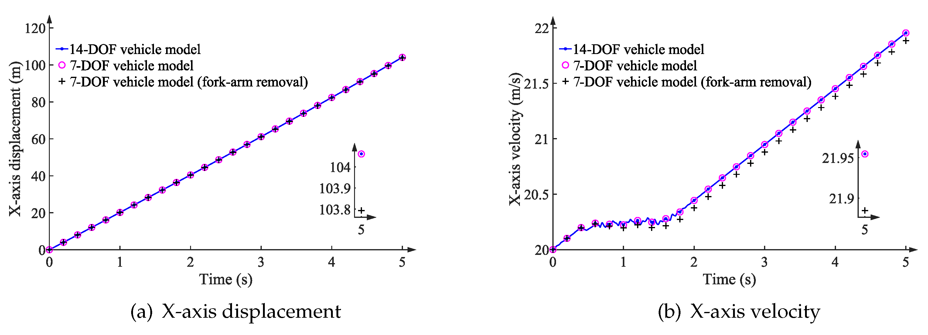
On each front wheel, a 300 Nm driving torque is applied, and the initial speed is 20 m/s. The simulation lasts 5 s and the time-step is 1 ms. Following dynamic simulations, the X- and Z-axis displacement and velocity, as well as the pitch angle and rate, are obtained for precision analysis. We compare the results of the proposed vehicle model with and without the fork-arm removal technique to those of the 14-DOF vehicle model (reference data). The comparative outcomes are depicted in Figure 9.

Due to the accumulation of numerical errors over time, the final displacement and velocity, as well as the pitch angle and rate, are used to quantify the accuracy of the solution. The results are shown in

Table 2. The numerical results after 5 s simulation (bumpy road).

Models	X-Axis (m and m/s)		Z-Axis (m and m/s)		Pitch (rad and rad/s)
	Displacement	Velocity	Displacement	Velocity	Angle	Rate
14-DOF	104.06	21.95	0.491	−4.03 × 10${}^{-4}$	−0.026	−9.36 × 10${}^{-4}$
7-DOF	104.06	21.95	0.491	−4.04 × 10${}^{-4}$	−0.026	−9.37 × 10${}^{-4}$
7-DOF (fork-arm removal)	103.79	21.88	0.491	−3.91 × 10${}^{-4}$	−0.026	−1.50 × 10${}^{-3}$

.

According to Figure 9 and Table 2, the greatest error occurs along the X-axis. The maximum displacement and velocity errors are 0.27 m and 0.07 m/s, corresponding to the reference values of 104.06 m and 21.95 m/s, respectively. The results along the Z-axis and around the Y-axis for the three vehicle multibody models are nearly identical when the vehicle traverses the bumpy road.

Dynamic maneuvers are simulated for 20 s with 1 ms time-step to determine the computational efficiency. The computational burden is in the state vector derivative function. C/C++ and Intel’s Math Kernel Library are utilized to implement numerical integration.

Table 3. Efficiency of different vehicle models in 20 s simulation (bumpy road).

	Vehicle Models
	14-DOF	7-DOF	7-DOF (Fork-Arm Removal)
CPU time (s)	7.436	4.806	4.921
Time saving		35.37% (↓)	33.82% (↓)

lists the elapsed CPU times for these three vehicle models.

Compared to the 14-DOF vehicle multibody model, the 7-DOF vehicle model improves computational efficiency by 35.37%, and the fork-arm removal technique increases efficiency by 33.82%. This is due to the reduction in both the size of dynamic equations and the number of loop-closure constrained equations.

4.2. Maneuver on a Sloping Road

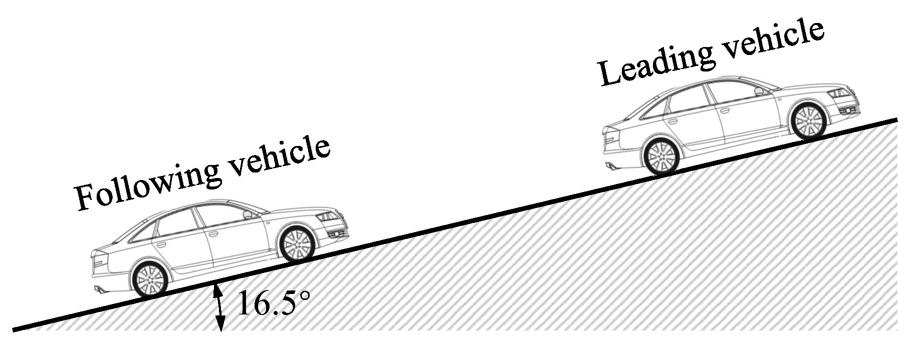
This section simulates a sloping road, which is a common driving environment for autonomous vehicles. Figure 10 depicts a road environment with a typical slope angle of 16.5°. An initial velocity of 15 m/s is used, and a 1550 Nm driving torque is imposed on the front wheels. For intelligent control to perform forward collision avoidance, adaptive cruise control, and platooning, in this ADAS environment, calculating the following vehicle’s states in real-time is anticipated. In addition, the vehicle’s vertical responses can be controlled to reduce vibration for improved riding quality.

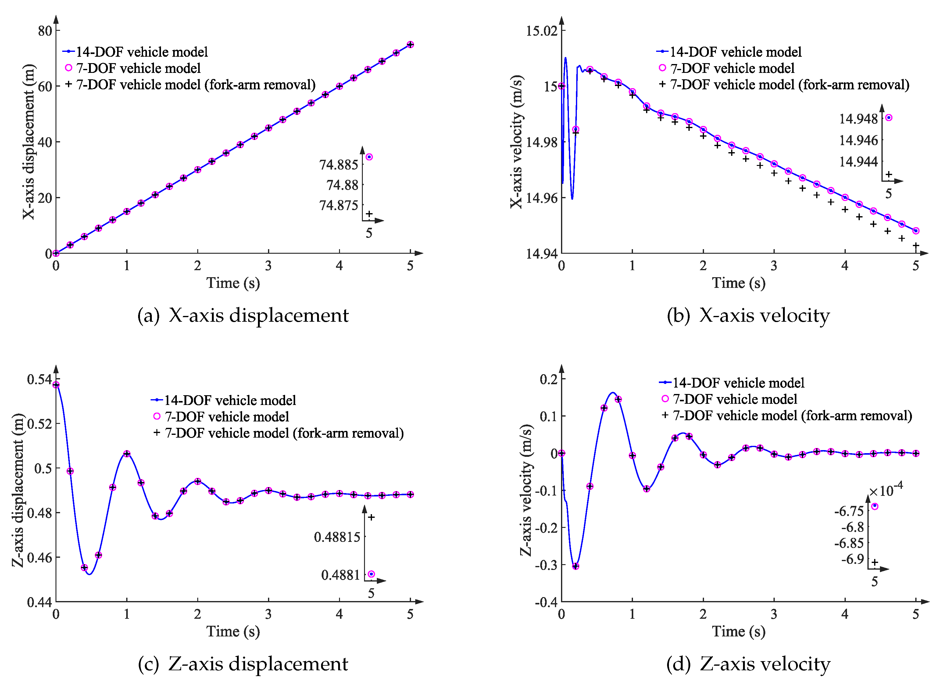
Within the three vehicle models, the displacement and velocity along the X- and Z-axes, as well as the pitch angle and rate, are calculated and compared. The comparative results are described in Figure 11.

Due to the accumulation of numerical errors over time, the final vehicle responses (states) are employed for accuracy analysis. The results are depicted in

Table 4. The numerical results after 5 s simulation (sloping road).

Models	X-Axis (m and m/s)		Z-Axis (m and m/s)		Pitch (rad and rad/s)
	Displacement	Velocity	Displacement	Velocity	Angle	Rate
14-DOF	74.89	14.95	0.4881	−6.73 × 10${}^{-4}$	−0.0367	7.08 × 10${}^{-4}$
7-DOF	74.89	14.95	0.4881	−6.7 4× 10${}^{-4}$	−0.0367	7.08 × 10${}^{-4}$
7-DOF (fork-arm removal)	74.89	14.94	0.4882	−6.91 × 10${}^{-4}$	−0.0367	6.86 × 10${}^{-4}$

From Figure 11 and Table 4, it can be seen that the maximum error occurs along the X-axis. The maximum errors of displacement and velocity are 0.014 m and 0.005 m/s, corresponding to the reference values of 74.89 m and 14.95 m/s, respectively. The results along the Z-axis and around the Y-axis when the vehicle traverses the sloping road are almost the same within the three vehicle multibody models.

The dynamic maneuvers are also simulated for 20 s with a 1 ms time-step to evaluate their effectiveness. The elapsed CPU times for the numerical integrations of the three vehicle models are presented in

Table 5. Efficiency of different vehicle models in the 20 s simulation (sloping road).

	Vehicle Models
	14-DOF	7-DOF	7-DOF (Fork-Arm Removal)
CPU time (s)	7.385	4.790	4.836
Time saving		35.14% (↓)	34.16% (↓)

.

The efficiency of the 7-DOF vehicle model is improved by 35.14% compared to the 14-DOF vehicle model, and by 34.16% when the fork-arm removal technique is applied.

4.3. Discussion

In the above ADAS environment, the results indicate that the fork-arm removal technique results in a slight decrease in efficiency. This is because the SDIFs couple the neighboring Cartesian accelerations via the mass matrix of the suspension lower-arm, as described in Equations (17) to (20). Moving the SDIFs to the LHS of the equations of motion complicates the generalized mass matrix. In turn, the sparse structure of the generalized mass matrix has been destroyed, resulting in an increase in computational burden.

Table 6. Efficiency of a 14-DOF vehicle model with and without the fork-arm removal technique in 20 s simulation.

Techniques	Road Environment
	Bumpy Raod	Sloping Road
Without fork-arm removal	7.436 s	7.385 s
With fork-arm removal	7.268 s (2.26% ↓)	7.237 s (2.00% ↓)

outlines the CPU time required to integrate a 14-DOF vehicle multibody model with and without the fork-arm removal technique on bumpy and sloping roads. The 4th-order Runge–Kutta integrator and 1 ms time-step are used for a fair comparison.

Applying the fork-arm removal technique to the multibody model of a 14-DOF vehicle yields a gain in efficiency of approximately 2%. As anticipated, the efficiency gain will increase for more complex vehicle systems, such as bus or truck systems, which contain more DOFs and fork-arm components. Due to the removal of fork-arm components, more bodies, joints, and constrained equations will be eliminated from the entire systems.

In addition, the fork-arm removal technique avoids accurate modeling of fork-arm component structures. It implies that only their dynamic properties are required for vehicle modeling, making implementation simple. This method is especially advantageous for larger closed-loop vehicle systems.

5. Conclusions

This work develops an accurate and real-time dynamics model for vehicle ADAS applications using a semi-recursive multibody formulation. This vehicle model efficiently describes the equations of motion using a small set of relative coordinates. In contrast to the simplified vehicle models used in most ADAS applications, the proposed vehicle model considers the dynamic properties of all components, resulting in accurate vehicle characteristics, such as pitch, roll, and yaw angles and their rates. Using the rod-removal method, a fork-arm removal technique is proposed to further reduce the size of dynamic equations and the number of loop-closure constrained equations. The dynamic simulations are performed on both bumpy and sloping roads to verify the effectiveness of the proposed vehicle model.

The results are examined in terms of X- and Z-axis displacement and velocity, as well as pitch angle and rate. Comprehensive studies demonstrate that the vehicle model provides accurate solutions for various road conditions. The CPU time for a 20 s dynamic simulation on bumpy and sloping roads is 4.806 s and 4.790 s, respectively. The respective efficiencies increased by 35.37% and 35.14% in comparison to the 14-DOF vehicle model. The proposed vehicle model can be used for simulations that are faster than real-time, yielding additional key characteristics that are difficult or impossible to measure using sensor networks. The proposed method for vehicle modeling is especially advantageous for ADAS applications in larger autonomous vehicles.