Driving Torque Control of Dual-Motor Powertrain for Electric Vehicles

Abstract

This paper investigates the driving torque control method for the dual-motor powertrain in electric vehicles (EVs) to achieve the performance of accurate vehicle speed tracking, seamless driving mode shift, and high energy efficiency. The configuration of the dual-motor powertrain is based on the parallel axle transmission structure, which does not contain any clutch or synchronizer. The powertrain provides three driving modes that are two single-motor driving modes and one dual-motor combined driving mode. A detailed dynamic model of the dual-motor powertrain is built to simulate the dynamic response of an EV. An energy management strategy (EMS) is used to select the driving mode and determine the ideal driving torque of two motors. The dynamic control strategy tries to track the ideal vehicle speed when uncertain parameters existed and avoid power interruption or impact during the mode shift. Three dynamic control strategies are proposed, which are the backward dynamic control strategy (BDCS), combined forward and backward dynamic control strategy (CFBDCS), and nested forward and backward dynamic control strategy (NFBDCS). The simulation results demonstrate that the NFBDCS has the best comprehensive performance in vehicle speed tracking, seamless mode shift, and good system energy efficiency.

1. Introduction

EVs have some new features and challenges, from energy and torque management to vehicle dynamics and control [1,2]. Among these challenges, the driving range limitation of EVs is the largest obstacle to their popularization. Introducing the multi-speed transmission or dual-motor layout into the powertrains of EVs can effectively improve the overall energy efficiency of EVs, which increases the driving range of EVs. At the same time, the higher energy efficiency leads to lower electric energy consumption and then contributes to the reduction of greenhouse gas emissions. Therefore, it is quite necessary to research the new powertrains for EVs.

Most EV powertrains use the configuration of a single motor with a one-speed transmission because of the high performance of electric motors. Electric motors can provide a constant torque from zero to base speed, and they can also achieve very high rotational speed, e.g., higher than 12,000 rpm. As a result, the single motor with a one-speed transmission can satisfy the demands of dynamic performance [3,4,5]. At the same time, this configuration represents a reduction of the drivetrain mass, volume, losses and cost, so it represents a cost-effective solution [6]. However, the power of the motor needs to be large enough to satisfy the dynamic performance requirement, which increases energy consumption. On the other hand, the one-speed transmission usually makes the motor work with low efficiency when the working conditions change, which further lowers the overall working efficiency of the motor so that the energy consumption increases.

Two types of powertrains are presented to improve the dynamic and economic performance of EVs, where the first type is the single motor with multi speed transmission, and the other type is the dual-motor powertrain. By replacing the one-speed transmission with a multi speed transmission, the dynamic performance of EVs can be improved, and this enables the motor to work in the high-efficiency regions, which improves the overall efficiency of the powertrain. Different types of multi-speed transmission equipped in EVs have been studied, including the continuously variable transmission (CVT) [7,8], automated manual transmission (AMT) [9,10], dual-clutch transmission (DCT) [11], and automatic transmission (AT) [12,13,14]. For the dual-motor powertrains, two downsized motors are used to replace the original single large-size motor. In this case, the torque utilization factor of the driving motor can be increased, and potentially the operating efficiency along driving cycles can be improved [15]. The dual-motor powertrains [16] can be realized with speed coupling or torque coupling mechanisms, which were termed in [17] as dual motor with planetary gear transmission (DMPGT) and dual motor with parallel axle transmission (DMPAT), respectively, or the combination of two coupling strategies, termed as compound dual-motor powertrain (CDMP) in [16,18,19]. The CDMP combines the priorities of the DMPGT and DMPAT to realize more driving modes, so it can improve the dynamic and economic performance of EVs further, but its configuration is more complicated. Hong et al. [20,21] proposed a new Simpson planetary gearset based dual-motor powertrain (SPGDMP), which can provide more driving modes, including four single-motor driving modes and two dual-motor driving modes, so it has higher dynamic and economic performance. More detailed configurations of dual-motor powertrains can be referred to in [22,23].

The gear shift or mode shift is an unavoidable operation in multi-speed transmissions and dual-motor powertrains. The dynamic control strategy during the gear shift and mode shift is quite important, otherwise a power interruption or large jerk may occur, which lowers the driving comfortability. To avoid this power interruption in the AMT, Sorniotti et al. [3] proposed a novel two-speed AMT, and a similar configuration was also proposed in [24,25]. Because the clutch is located at the rear of the transmission in the new layout of the two-speed AMT, it can realize a seamless gear shift through suitable control of the driving motor and actuation of the clutch. Three alternative gearshift control systems were outlined by [3], with particular reference to the typical characteristics of electric powertrains, which required particular control algorithms for the seamless management of the upshifts. Hu et al. [26] investigated the effects of the shift control parameters of the synchronizer, including the gear shifting force, relative speed difference, and relative rotation angle, in clutchless AMTs on shifting impact. Tian et al. [27] combined the synchronizer with a planetary gear to propose a new two-speed transmission used in EVs. Polynomials with different order were employed to formulate the motor torque and speed trajectories. Besides the traditional synchronizer, Mo et al. [28] investigated a new Harpon shift synchronizer-based AMT in EVs, in which a spring force is used to replace the friction force in traditional synchronizers to implement the speed synchronization process. Although the new synchronizers and control methods can reduce the gear shift time or vehicle jerk, the power interruption cannot be avoided due to the limitation of the principle of the AMT. To avoid the power interruption, the AT and DCT are used widely.

Roozegar et al. [29] developed a gear shifting control scheme for the two-speed AT in EVs. A two-phase control was proposed for shifting between each of the two gear ratios, which guaranteed a smooth and swift shift. Two independent PID controllers were employed to realize the shifting between each gear pair. In [30], the Pontryagin Minimum Principle was applied to design an optimal shifting controller of a two-speed AT. This controller kept the output speed and output torque of the driveline constant during the gear shifting operation while minimizing the shifting time and the dissipation of energy caused by the internal brakes. Fang et al. [31] used the optimal control method to produce the target motor torque, clutch torque and brake torque, while trying to minimize vehicle jerk and frictional work during the gear shift. Tian et al. [32] proposed a two-speed AT and its dynamic control strategy in gear shifting. Through controlling the variation of motor torque and brake torque during the torque phase and inertia phase in different ways, three control strategies were proposed to implement the power-on gear shift, leading to different vehicle jerk and frictional work.

Zhu et al. [33] investigated the gear shifting control strategy of EVs equipped with a two-speed DCT, in which both the simulation and experimental results were provided to demonstrate the shift transient behavior. Walker et al. [34] developed a series of power-on and power-off shifting control strategies for the two-speed DCT based EVs. Through controlling the clutch torque and motor torque in the torque phase and inertia phase, the power interruption and large impact could be reduced. A smooth gear shifting control structure for DCTs was developed in [35]. The control structure is divided into two levels, where the upper level governs the procedure to determine the most suitable torque trajectories of the clutches and power source, and the lower level manages the strategy for each actuator controller to track the given torque trajectories. Li et al. [36] designed an optimal control strategy for gear shifting in DCTs to achieve a smooth shifting process.

The gear shift process of single-motor-based multi-speed transmissions generally contains two phases that are the torque phase and inertia phase. To realize a smooth gear shift, the motor torque and clutch/brake torque should be coordinately controlled in both of the two phases, which is indeed a complicated control process and even unachievable sometimes, e.g., the clutch torque cannot be in the same direction as its rotational direction. With dual-motor powertrains it is easy to realize a smoother gear/mode shift without relying on the precise control of clutch/brake torque since the motor torque can be easily controlled. Liang et al. [37] investigated the gear shift control strategy of a dual-motor powertrain with a three-speed parallel axle transmission, which uses the second motor to complement the driving torque during the gear shift. However, the synchronizer is simplified to a friction model, which artificially improves its shift performance. To reduce jerk induced by the mode shift, Zhang et al. [38] presented a stage-by-phase multivariable combination controller based on the control of the position, velocity, and force of the actuators, to implement the mode shift of a dual-motor centralized and distributed coupling drive system. The simulation and experiment results demonstrated that the vehicle jerk can be reduced to lower than 10 m/s³ by using the combination controller. Wu et al. [39] proposed a mode shift control strategy for the planetary gear-based dual-motor powertrain, where the polynomials trajectory of the motor’s speed is formulated during the mode shift and then the motor’s torque is controlled by the PI controllers to track the ideal speed trajectory. The simulation results demonstrated that the vehicle jerk is extremely small, but the mode shift control strategy only depends on the control of the motors without considering the influence of the brakes, which leads to a deviation from the practical case. Hu et al. [16] investigated the mode shift control strategy of a CDMP, in which the maximum vehicle jerk could be reduced to 6 m/s³. Wu et al. [40] proposed a seamless mode shift control strategy for a SPGDMP by decoupling the mode transition process to torque transtiont process and speed transition process, which reduces the control difficulty. The smooth step function is used to produce the transition trajectories of torque and speed, and the vehicle jerk during the mode shift is controlled to be lower than 2 m/s³.

Most of the multi-speed transmission and dual-motor powertrains use the clutch or brake to reduce the power interruption or impact in the gear shifting or mode shifting process, but the hydraulic system of clutch and brake produces non-negligible energy loss, which lowers the transmission efficiency. At the same time, a coordination control strategy for the motors and clutches or brakes is required, which increases the control difficulty. To improve both energy efficiency and driving comfort, this paper investigates the dynamic control strategy to implement the seamless mode shift for DMPAT without using any shifting mechanism but only controlling the torque of the two driving motors. We propose a nested forward and backward dynamic control strategy, which tries to track the ideal vehicle speed when uncertain parameters exist, and to avoid power interruption or impact during the mode shift. In Section 2, the layout and dynamic model of DMPAT will be provided, following with the energy management strategy presented in Section 3. The dynamic control strategies of vehicle speed tracking and seamless mode shift will be proposed in Section 4. The simulation results of drivability and economy based on the proposed dynamic control strategies are provided in Section 5. Some conclusions are given in the last section.

2. Dynamic Modelling of the EV Powertrain

2.1. Layout of the Dual-Motor Powertrain

The layout of a powertrain with a DMPAT is shown in Figure 1 [17], where the main components are two driving motors, EM1 and EM2, three reduction gear pairs, and the differential gear. The EM1 outputs the driving torque through gear 1 (with gear ratio n₁) and final gear (with gear ratio n₃) to the vehicle, while the EM2 outputs its driving torque through gear 2 (with gear ratio n₂) and the final gear to the vehicle. It is worth noting that there is neither clutch nor synchronizer in the powertrain, so the two motors always have a connection with the vehicle. The powertrain can provide three driving modes by turning on or turning off the two motors. The three driving modes are named as Mode 1, Mode 2, and Mode 1 & 2. In Mode 1, only the EM1 provides torque to drive the vehicle while the EM2 does not output torque since it is off. On the contrary, EM1 is off while EM2 is on for Mode 2. Mode 1 & 2 is the dual-motor combined driving mode, so both EM1 and EM2 output torque to the vehicle simultaneously. When the vehicle-requested torque is small or moderate, the powertrain works in Mode 1 or Mode 2, which makes the powertrain have higher energy efficiency. When the required torque of the vehicle is quite large, the powertrain works in Mode 1 & 2, which can output larger torque to satisfy the dynamic performance.

Motor characteristics are usually described by an efficiency map, but the efficiency map has a blank region when the motor torque and speed are low. To solve this problem, the efficiency map is transferred to a power loss map. The detailed method of computing the power loss map from the efficiency map can be referred to in [17]. The power distribution between EM1 and EM2 and the gear ratios of the transmission have an effect on both the dynamic performance and energy efficiency of EVs. The parameters shown in [17], having a good trade-off between dynamic performance and energy efficiency, will be used in this paper. The power loss maps of EM1 and EM2 are shown as Figure 2, in which the red curves denote the maximum output torque of motors changing with the rotational speed. It is worth noting that when the motor is off, its power loss is almost zero. The peak power of EM1 and EM2 are respectively 65 kW and 35 kW, and their power loss maps have similar shapes but different magnitudes.

2.2. Dynamic Model of the Powertrain

2.2.1. Motor Model

The motor model simulates the motor’s torque response and updates the motor’s maximum output-torque limit according to the motor speed, as well as computes the current power loss. The power loss of the motor is obtained by using a lookup table from the power loss maps shown in Figure 2. The main task of this paper is to research the dynamic control strategy of vehicle speed tracking and mode shift, so for convenience the motor torque is modelled by a first-order delay transfer function [41], expressed as

$$T_i\left(s\right)=1/(1+{\tau }_{i}s), i=1,2$$

(1)

where τ_i denotes the time delay constant, which is considered to be 10 ms in this paper.

2.2.2. Transmission Model

To simplify the problem, a five degrees of freedom (DOF) model is used to build the transmission model and then simulate the mode shifting process. Figure 3 shows the transmission model, the 5 DOFs of which are the rotational displacement of the two motors denoted by θ₁ and θ₂ the rotational displacement of the main reduction gear, final gear, and wheel, denoted by θ₃, θ₄, and θ₅ respectively. The inertia of the two motors is I₁ and I₂; the inertia of the main reduction gear pair is noted by I_3a, I_3b, and I_3c; the final reduction gear pair inertia is denoted by I_4a and I_4b; and the vehicle equivalent inertia is noted by I₅. There are four elastic shafts connecting the five components, and the elastic shafts are modelled by the torsional spring and damper with stiffness K_i and damping ratio C_i, i = 1, 2, 3, and 4. The gear pairs are considered to be rigid body and the teeth backlash is neglected. The corresponding parameters are shown in

Table 1. Parameters of the powertrain and vehicle.

Stiffness (Nm/rad)				Inertia (kgm2)
K1	K2	K3	K4	I1	I2	I3a	I3b	I3c	I4a	I4b	I5
50,000	50,000	20,000	40,000	0.02	0.02	0.002	0.005	0.002	0.002	0.005	124.11
Damping ratio (Nms/rad)				Gear ratio (-)			Vehicle parameters
C1	C2	C3	C4	n1	n2	n3	mV (kg)	AV (m2)	Cd (-)	Ct (-)	RW (m)
1	1	1	2	1.2	2.8	3	1379	2.5826	0.25	0.015	0.3

. There are three external torques actuated on the system, where T₁ and T₂ are the motor output torques, while T₅ denotes the equivalent vehicle load torque.

Based on Figure 3, the dynamic equation of the transmission system is given as follows

$$I\ddot{\mathsf{\theta }}+C\dot{\mathsf{\theta }}+K\mathsf{\theta }=T$$

(2)

where

$$\begin{array}{l}I=\left[\begin{array}{ccccc}{I}_1& 0& 0& 0& 0\\ & I_2& 0& 0& 0\\ & & \begin{array}{l}{n}_1^2{I}_{3a}+\\ n_2^2{I}_{3c}+I_{3b}\end{array}& 0& 0\\ & & & n_3^2{I}_{4a}+I_{4b}& 0\\ \mathrm{symmetric}& & & & I_5\end{array}\right], C=\left[\begin{array}{ccccc}{C}_1& 0& -n_1{C}_1& 0& 0\\ & C_2& -n_2{C}_2& 0& 0\\ & & \begin{array}{l}{n}_1^2{C}_1+\\ n_2^2{C}_2+C_3\end{array}& -n_3{C}_3& 0\\ & & & n_3^2{C}_3+C_4& -C_4\\ \mathrm{symmetric}& & & & C_4\end{array}\right],\\ K=\left[\begin{array}{ccccc}{K}_1& 0& -n_1{K}_1& 0& 0\\ & K_2& -n_2{K}_2& 0& 0\\ & & \begin{array}{l}{n}_1^2{K}_1+\\ n_2^2{K}_2+K_3\end{array}& -n_3{K}_3& 0\\ & & & n_3^2{K}_3+K_4& -K_4\\ \mathrm{symmetric}& & & & K_4\end{array}\right], \mathsf{\theta }=\left[\begin{array}{c}{\theta }_1\\ {\theta }_2\\ {\theta }_3\\ {\theta }_4\\ {\theta }_5\end{array}\right], T=\left[\begin{array}{c}{T}_1\\ T_2\\ 0\\ 0\\ T_5\end{array}\right]\end{array}$$

(3)

Here I is the inertia matrix, C is the damping matrix, K denotes the stiffness matrix, θ is the state vector, and T is the load vector. The equivalent vehicle load torque T₅ is determined by the vehicle model shown in the following content.

2.2.3. Vehicle Model

The load of the cruising vehicle is expressed by the following equation

$$T_5=F_V{R}_W, F_V=m_{V}g\sin \phi +\frac{1}{2}\rho A_V{C}_d{v}^2+m_{V}g{C}_t\cos \phi$$

(4)

where F_V is the resistance induced by the incline of the road, aerodynamic drag, and tire rolling resistance, m_V is the mass of the vehicle, g denotes gravity acceleration, φ is the incline angle of the road, ρ is the air density, A_V is the frontal area of vehicle, C_d denotes the drag coefficient, C_t denotes the tire rolling friction coefficient, R_W is the tire radius, and v is the vehicle speed. Due to the vehicle load being a resistant torque, the negative symbol of T₅ should be added when Equation (4) is submitted to Equation (2). The values of these parameters are shown in Table 1.

3. Energy Management Strategy of the Dynamic System

An EMS is used to produce the ideal driving torque of the two motors through optimizing the energy efficiency of a dynamic system after the driving condition is given, i.e., vehicle speed and acceleration are provided. To make the computational time of optimization acceptable, the backward-facing dynamic model is usually employed to build the constraints. In the optimization, the design variable is discretized to a dense grid and the optimal node of the grid is considered as the optimal solution, which is almost the global optimal solution.

3.1. Backward-Facing Dynamic Model of the Powertrain

To guarantee real-time control, a backward-facing dynamic model is employed to develop the EMS, due to its lower computational cost. In the backward-facing dynamic model, the shafts are considered to be rigid body, so there will be only 1 DOF. After the elastic forces are neglected, the dynamic equation of system is given as follows

$$\left(n_1^2{n}_3^2(I_1+I_{3a})+n_2^2{n}_3^2(I_2+I_{3c})+n_3^2(I_{3b}+I_{4a})+I_{4b}+I_5\right)\frac{\dot{v}}{R_W}=n_1{n}_3{T}_1+n_2{n}_3{T}_2-T_5$$

(5)

The rotational speed of the two motors is proportional to the vehicle speed, so the speed constraint of the system is expressed by

$${\omega }_1=n_1{n}_3\frac{v}{R_W}, {\omega }_2=n_2{n}_3\frac{v}{R_W}$$

(6)

where ω₁ and ω₂ are the rotational speed of EM1 and EM2.

Once the vehicle speed is given, both the rotational speed of EM1 and EM2 can be determined by Equation (6). However, for the torque, Equation (5) contains only one constraint but two variables, i.e., T₁ and T₂. There will be uncountable combinations of T₁ and T₂ to satisfy the Equation (5), so the EMS should be used to select the optimal combination of motor torques.

3.2. Optimization Model of the EMS

The robust EMS proposed in [42] will be used to optimize the torque distribution of the two motors. The optimization model is expressed as the following equation

$$\begin{gathered} \underset{T_1}{\min } {\tilde{P}}_M\left(T_1,T_2,{\omega }_1,{\omega }_2\right)=k^{-sign(P_M)}{P}_M\left(T_1,T_2,{\omega }_1,{\omega }_2\right) \\ \begin{array}{cc} \mathrm{s}. \mathrm{t}. \hfill & \mathrm{Equations} \left(5\right) and \left(6\right)\hfill \\ \hfill & P_M\left(T_1,T_2,{\omega }_1,{\omega }_2\right)=T_1{\omega }_1+{\mathit{P\_loss}}_1\left(T_1,{\omega }_1\right)+T_2{\omega }_2+{\mathit{P\_loss}}_2\left(T_2,{\omega }_2\right)\hfill \\ \hfill & k\left(\Delta T_1\right)=\{\begin{array}{c}1,\Delta T_1\le 100\Delta t\hfill \\ 0.95,\Delta T_1>100\Delta t\hfill \end{array},\Delta T_1=\left|T_1(t)-T_1(t-\Delta t)\right|\hfill \\ \hfill & -{\omega }_{\max 1}\le {\omega }_1\le {\omega }_{\max 1};-T_{\max 1}\left({\omega }_1\right)\le T_1\le T_{\max 1}\left({\omega }_1\right)\hfill \\ \hfill & -{\omega }_{\max 2}\le {\omega }_2\le {\omega }_{\max 2};-T_{\max 2}\left({\omega }_2\right)\le T_2\le T_{\max 2}\left({\omega }_2\right)\hfill \end{array} \end{gathered}$$

(7)

where P_M is the consumed power of the two driving motors, the P_loss₁ and P_loss₂ are the lost power of the two motors obtained from the power loss maps shown in Figure 2, k is a penalty factor to avoid frequent mode shifting operation, ΔT₁ denotes the torque variation of EM1 between the last call of the EMS and the current call of the EMS, and Δt is the calling period of the EMS. To guarantee the real-time control of the EMS, the calling period of the EMS cannot be too short, while to improve the energy efficiency performance it may not be too long. As a result, Δt can be set as different values based on the computational capability of the practical control unit. The optimization model uses the torque of EM1 as the design variable because the torque of EM2 can then be determined by Equation (5) and the speed of the two motors can be determined by Equation (6). Given the driving cycle, the optimal torque distribution between the two motors can be obtained by solving Equation (7). When T₂ = 0 and T₁ ≠ 0, the driving mode is Mode 1, and on the contrary, the driving mode is Mode 2. When both T₁ and T₂ are nonzero, the driving mode is Mode 1 & 2.

Using the previous optimization model to simulate the NEDC driving cycle, the torque distribution between the two driving motors and the driving modes are shown as Figure 4, in which the value of Mode 1, 2, and 3 denotes the Mode 1, Mode 2, and Mode 1 & 2, respectively. It can be found that most of the time the vehicle is driven in Mode 2, in which T₁ is 0 and the EV is driven by T₂. Only in the end of the driving cycle is the vehicle driven in Mode 1 and Mode 1 & 2, so T₁ becomes nonzero in these periods. There are two periods driven by Mode 1 that are around 1100 s and 1120 s, and Mode 1 & 2 happens in three periods that are between 1090 s and 1100 s, around 1122 s, and around 1125 s. When the EM2 can provide the power needed by the vehicle, the EMS only makes EM2 work, because the electrical power loss of EM1 can be avoided compared to the combined driving mode. Generally, the single-motor driving mode has less power loss than the combined driving mode because they have the same mechanical power loss, but the latter has an additional electrical power loss induced by the other motor. When the power demand increases, the EMS makes EM1 work harder, or both EM1 and EM2 work simultaneously, which can meet dynamic requirements. When the driving mode is changed, the torque of EM1 and EM2 is required to be well-controlled to avoid power interruptions and large impacts, which will be investigated in the following section.

4. Dynamic Control Strategies of the DMPAT

A good dynamic control strategy should track the ideal vehicle speed and ideal torque provided by the EMS. At the same time, it is expected to reduce the power interruption or impact during mode shift. Three dynamic control strategies are proposed in this section to control the driving torque of EM1 and EM2. The first one is to use the torque signal provided by the EMS to control the two motors directly. Since the EMS is based on the backward-facing dynamic model, it is named as a backward dynamic control strategy (BDCS). The second one employs a PI controller to control one motor to track the vehicle speed and the other motor is directly controlled by the torque signal provided by the EMS. The PI controller is used in the forward-facing dynamic model, so this control strategy is termed as a combined forward and backward dynamic control strategy (CFBDCS). The third control strategy uses a nested control configuration, where the first level is a PI controller to control the total torque actuated on the vehicle and the second level is the EMS distributing the torque between the two motors, so it is termed as a nested forward and backward dynamic control strategy (NFBDCS).

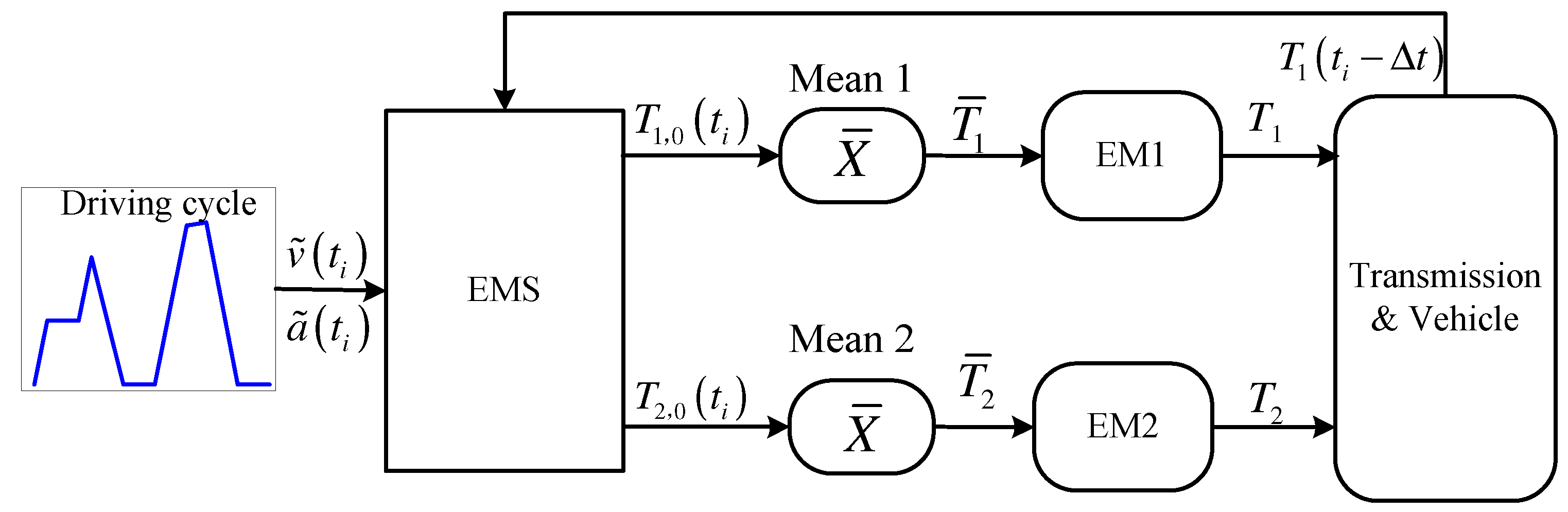
4.1. Backward Dynamic Control Strategy

The schematic of BDCS is shown in Figure 5, which contains the driving cycle model, EMS, two motor models, transmission and vehicle model shown in Section 2.2, and two mean operation models.

The ideal vehicle speed $\tilde{v}$ and acceleration $\tilde{a}$ are produced by the given driving cycle in the simulation. For practical driving, the ideal vehicle speed and acceleration can be obtained by the driver’s pedal signal. The EMS shown in Section 3 is based on the backward model, so it only computes the motor torque after the ideal vehicle speed and acceleration are provided. EMS is based on the backward-facing dynamic model, so the torque obtained from the EMS is named as backward torque in this paper. The EMS is called once per period of Δt to implement the real-time control. As a result, the EMS outputs the step changing backward torque of EM1 and EM2 with step length Δt, noted by T_1,0(t_i) and T_2,0(t_i). To avoid the step change of backward torque, the mean operation $\overline{X}$ over a running window with the time width of Δt is added after the backward torque signal, which makes the backward torque continuous, noted by ${\overline{T}}_1$ and ${\overline{T}}_2$, i.e.,

$${\overline{T}}_1=\frac{1}{\Delta t}{\displaystyle {\int }_{t_i-\Delta t}^{t_i}{T}_{1,0}\left(t\right)dt}, {\overline{T}}_2=\frac{1}{\Delta t}{\displaystyle {\int }_{t_i-\Delta t}^{t_i}{T}_{2,0}\left(t\right)dt}$$

(8)

The motors models transfer the continuous backward torque control signal to the practical torque, which is then input to the transmission and vehicle model. The schematic of mode shifting (from Mode 1 to Mode 2) based on the BDCS is shown in Figure 6, where T₃ denotes the torque acting on the 3rd shaft, defined in Equation (11). The structure of the BDCS is quite simple, but it does not contain any feedback on speed. This lowers the vehicle speed tracking performance when uncertain parameters exist in the dynamic model.

4.2. Combined Forward and Backward Dynamic Control Strategy

The BDCS is quite simple, but it is easily disturbed by uncertain parameters. To overcome this weakness, a PI controller is added in the control system which adjusts the motor torque based on the difference between the ideal vehicle speed and the actual speed. Since there are two motors in the powertrain, one motor will be used to track the ideal vehicle speed, while the other motor will provide the backward torque determined by the EMS. In Mode 1, the backward torque of EM2 is fixed to zero, so EM1 will be used to track the ideal vehicle speed. On the contrary, the backward torque of EM1 equals zero in Mode 2, so EM2 will be used to track the ideal vehicle speed. In Mode 1 & 2, the backward torque of both EM1 and EM2 is nonzero, so either EM1 or EM2 can be used to track the ideal vehicle speed, while the other motor is used to provide the backward torque. In this paper, EM1 is used to track the ideal vehicle speed in Mode 1 & 2, and EM2 is used to track the backward torque, so it has the same control strategy as Mode 1. As a result, the dynamic control strategy only considers the shift from Mode 1 to Mode 2.

The control scheme of CFBDCS is shown in Figure 7, which adds a PI controller, two switches and two gains, compared to the control scheme of the BDCS. $\widehat{T}$ represents tracking torque, which is computed by the following equation based on the definition of the PI controller

$$\widehat{T}=Pe+I{\displaystyle {\int }_0^{t}edt}, e=\tilde{v}-v$$

(9)

After tuning the parameters, the PI controller parameters are set as P = 210 and I = 1.68 in this paper. The two gains are set as the reciprocal of gear ratio n₁ and n₂, which makes the two motors have the same tracking torque actuated on the vehicle.

Based on the value of the mode output by the EMS, the two switches can select the control signal of the two motors between the backward torque and tracking torque. When the Mode = 2, EM1 outputs the backward torque and EM2 outputs the tracking torque; when the Mode = 1, EM1 outputs the tracking torque and EM2 outputs the backward torque. The mathematical model of the two switches is expressed by the following equation.

$${\tilde{T}}_1=\{\begin{array}{l}{\widehat{T}}_1=\widehat{T}/n_1,\mathrm{Mode}=1\\ {\overline{T}}_1, \mathrm{Mode}\ne 1\end{array}, {\tilde{T}}_2=\{\begin{array}{l}{\overline{T}}_2, \mathrm{Mode}=1\\ {\widehat{T}}_2=\widehat{T}/n_2, \mathrm{Mode}\ne 1\end{array}$$

(10)

The CFBDCS can track the vehicle speed quickly and also accurately follows the backward torque determined by the EMS. However, a large impact may occur in the mode shifting process. When the driving mode is being changed, the two switches in Figure 7 are actuated. Considering the case of Mode 1 changing to Mode 2, the schematic of the torque variation during the shifting process is shown in Figure 8.

Before the time t₀, the EV is driven in Mode 1, and it is then driven in Mode 2 after the time t₀. As expressed in the last subsection, there is a step change for the discrete backward torque T_1,0(t_i) and T_2,0(t_i), which are transformed to the continuous backward torque ${\overline{T}}_1$ and ${\overline{T}}_2$. The tracking torque ${\widehat{T}}_1$ and ${\widehat{T}}_2$ are produced by the PI controllers, so they are continuous and have a fixed proportional relation. The T₃ denotes the torque actuated on the 3rd shaft, expressed by

$$T_3=n_1{\tilde{T}}_1+n_2{\tilde{T}}_2$$

(11)

Here the inertia torque of components and the elasticity of the shafts are neglected. In Mode 1, the output torque of the EM1 is the tracking torque ${\widehat{T}}_1$ based on Equation (10), while EM2 outputs the continuous backward torque which equals zero. In Mode 2, the EM1 outputs the continuous backward torque ${\overline{T}}_1$ while EM2 outputs the tracking torque ${\widehat{T}}_2$. If the switching operation is finished instantaneously, we can obtain T₃ shown in Figure 8 by substituting Equation (10) with Equation (11). It can be found that there is a large step change for T₃, which may bring a large impact to the vehicle.

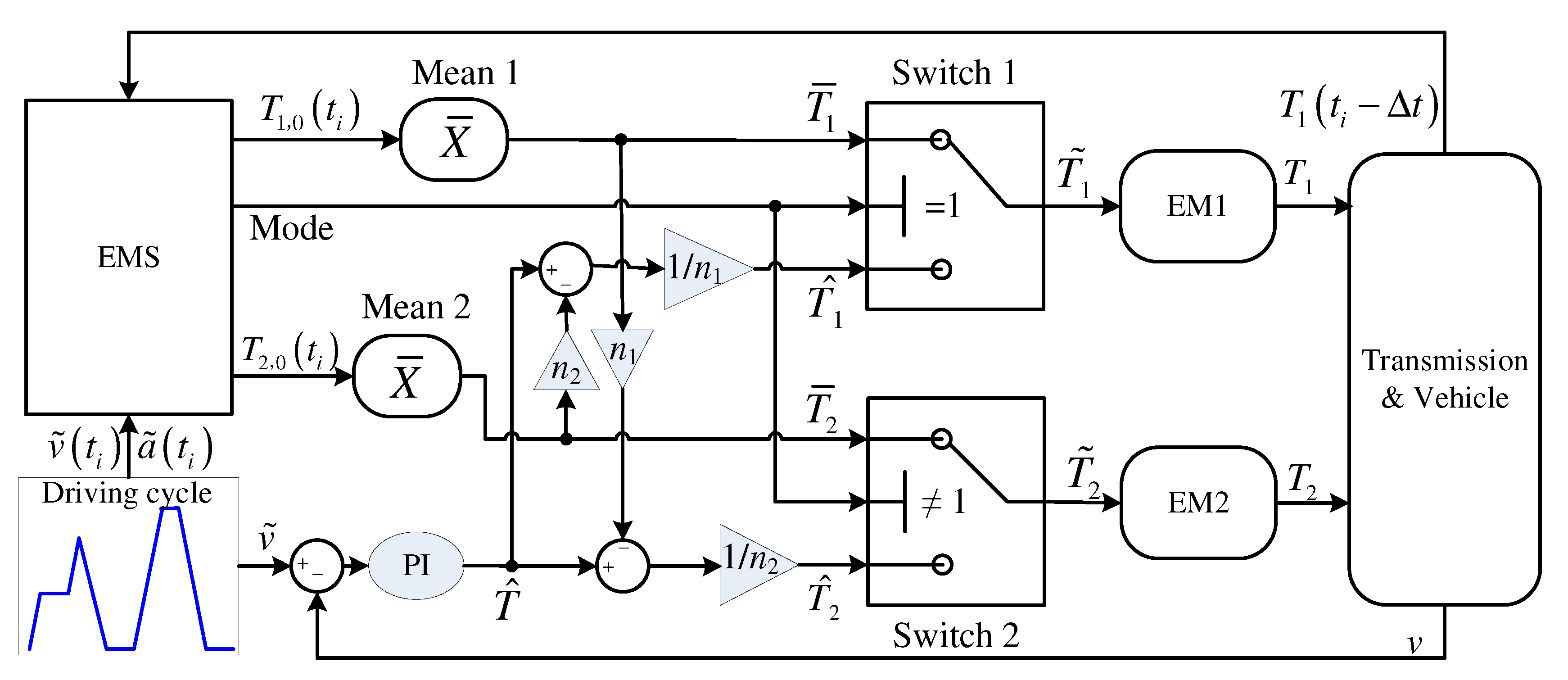
4.3. Nested Forward and Backward Dynamic Control Strategy

In the NFBDCS, the total driving torque actuated on the vehicle is controlled by the PI controller, which can avoid the torque step change of T₃, so as to avoid a large impact in the mode shifting process. After the total torque $\widehat{T}$ is produced by the PI controller, the EMS is used to distribute the torque between the two motors. The control scheme of NFBDCS is shown in Figure 9.

The tracking torque is expressed by

$${\widehat{T}}_1=\frac{\widehat{T}-n_2{\overline{T}}_2}{n_1}, {\widehat{T}}_2=\frac{\widehat{T}-n_1{\overline{T}}_1}{n_2}$$

(12)

Substituting Equation (12) into Equations (10) and (11), the torque actuated on the 3rd shaft is expressed by

$$T_3=\{\begin{array}{c}{n}_1{\widehat{T}}_1+n_2{\tilde{T}}_2=\widehat{T}-n_2{\overline{T}}_2+n_2{\overline{T}}_2=\widehat{T}, \mathrm{Mode}=1\\ n_1{\tilde{T}}_1+n_2{\widehat{T}}_2=n_1{\overline{T}}_1+\widehat{T}-n_1{\overline{T}}_1=\widehat{T}, \mathrm{Mode}\ne 1\end{array}$$

(13)

From this equation it can be found that no matter what the driving mode is, T₃ is always equal to the torque $\widehat{T}$ produced by the PI controller, which cancels the large impact in the mode shifting process.

Figure 10 shows the schematic of the torque variation during the mode shift. It can be found that no torque step change happened for T₃, which is quite smooth, so the shifting process is seamless. From Figure 10, although T₃ does not contain a step change, the ${\tilde{T}}_1$ and ${\tilde{T}}_2$ still contain a step change. This step change does not produce an impact on the vehicle, but it has an effect on the two motors, so it also should be avoided. To cancel the step change, a transition process is added between two modes. Still considering the case of mode shifting from Mode 1 to Mode 2, the duration of the transition process is set as the calling period of EMS Δt. In this period, the torque of EM1 changes from ${\widehat{T}}_1(t_0)$ to $T_{1,0}(t_0^{+})$ linearly, while the torque of EM2 is used to compensate for the changes in EM1′s torque, expressed by

$${\tilde{T}}_1\left(t\right)={\widehat{T}}_1(t_0)+\frac{\left(t-t_0\right)}{\Delta t}\left(T_{1,0}(t_0^{+})-{\widehat{T}}_1(t_0)\right), {\tilde{T}}_2=\frac{\widehat{T}-n_1{\tilde{T}}_1}{n_2}, t_0\le t\le t_0+\Delta t$$

(14)

Using Equation (14) to implement the transition process, the torque variation in the mode shift is shown in Figure 11. Similarly, when Mode 2 is changed to Mode 1, the torque in the transition process can be expressed by

$${\tilde{T}}_2\left(t\right)={\widehat{T}}_2(t_0)+\frac{\left(t-t_0\right)}{\Delta t}\left(T_{2,0}(t_0^{+})-{\widehat{T}}_2(t_0)\right), {\tilde{T}}_1=\frac{\widehat{T}-n_2{\tilde{T}}_2}{n_1}, t_0\le t\le t_0+\Delta t$$

(15)

The control scheme of Mode 1 & 2 is absolutely equivalent to that of Mode 1, so there is no need for mode shifting control between the Mode 1 & 2 and Mode 1, and the mode shifting process between Mode 1 & 2 and Mode 2 is the same as the mode shifting process between Mode 1 and Mode 2.

5. Simulation Results

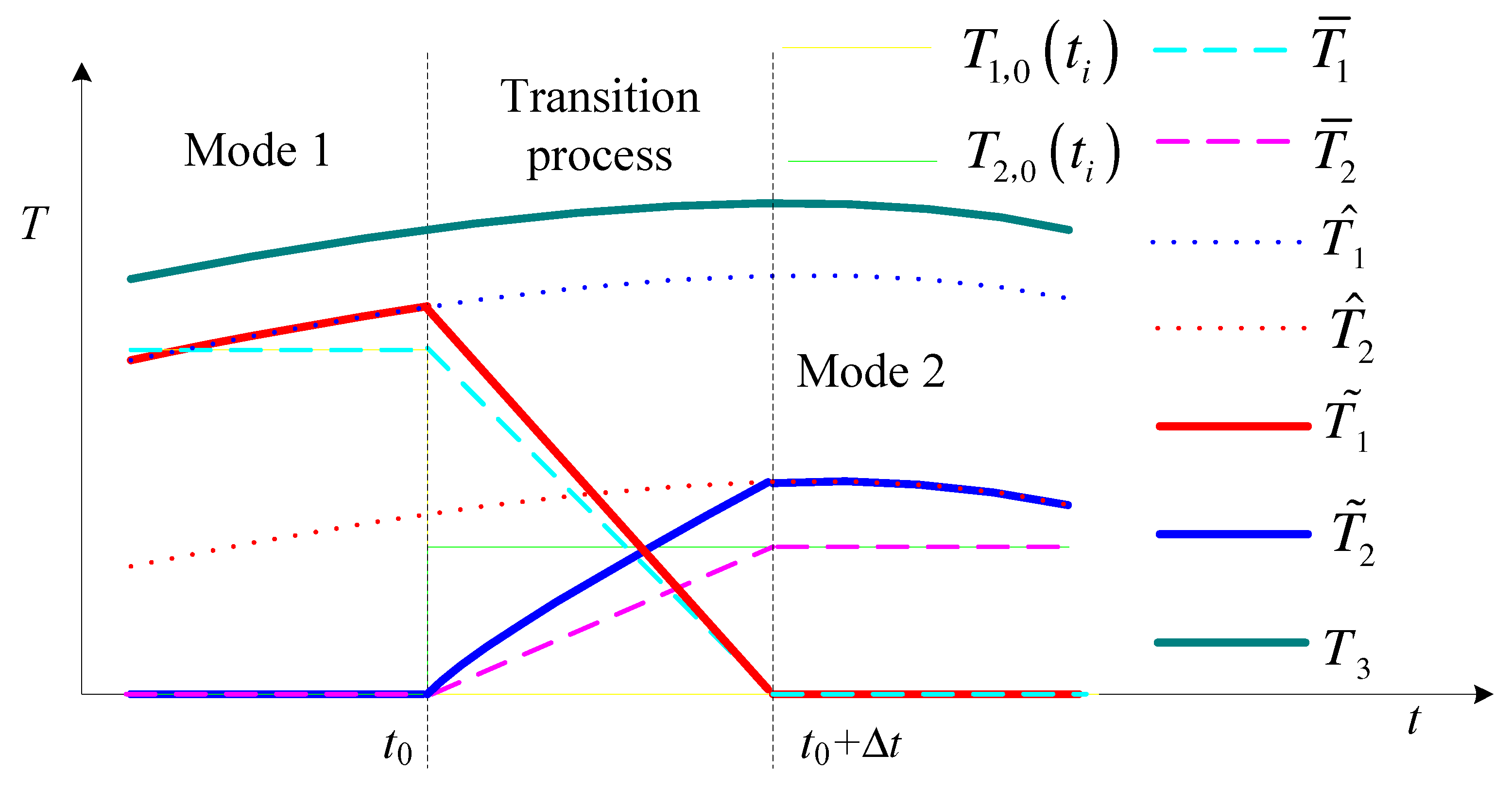
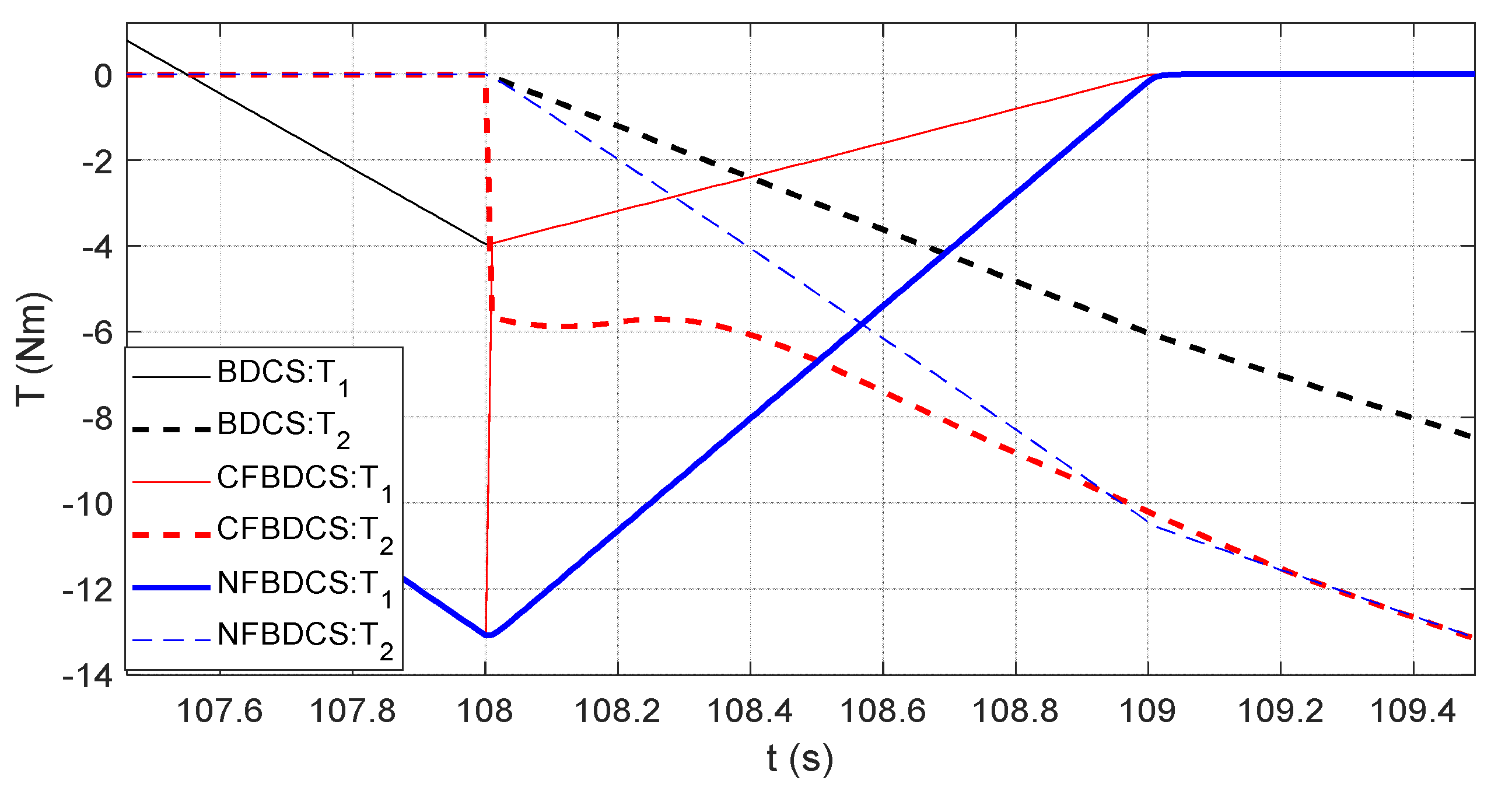
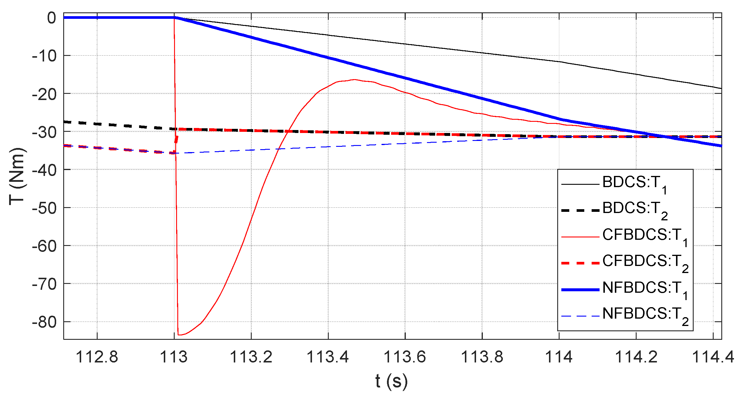
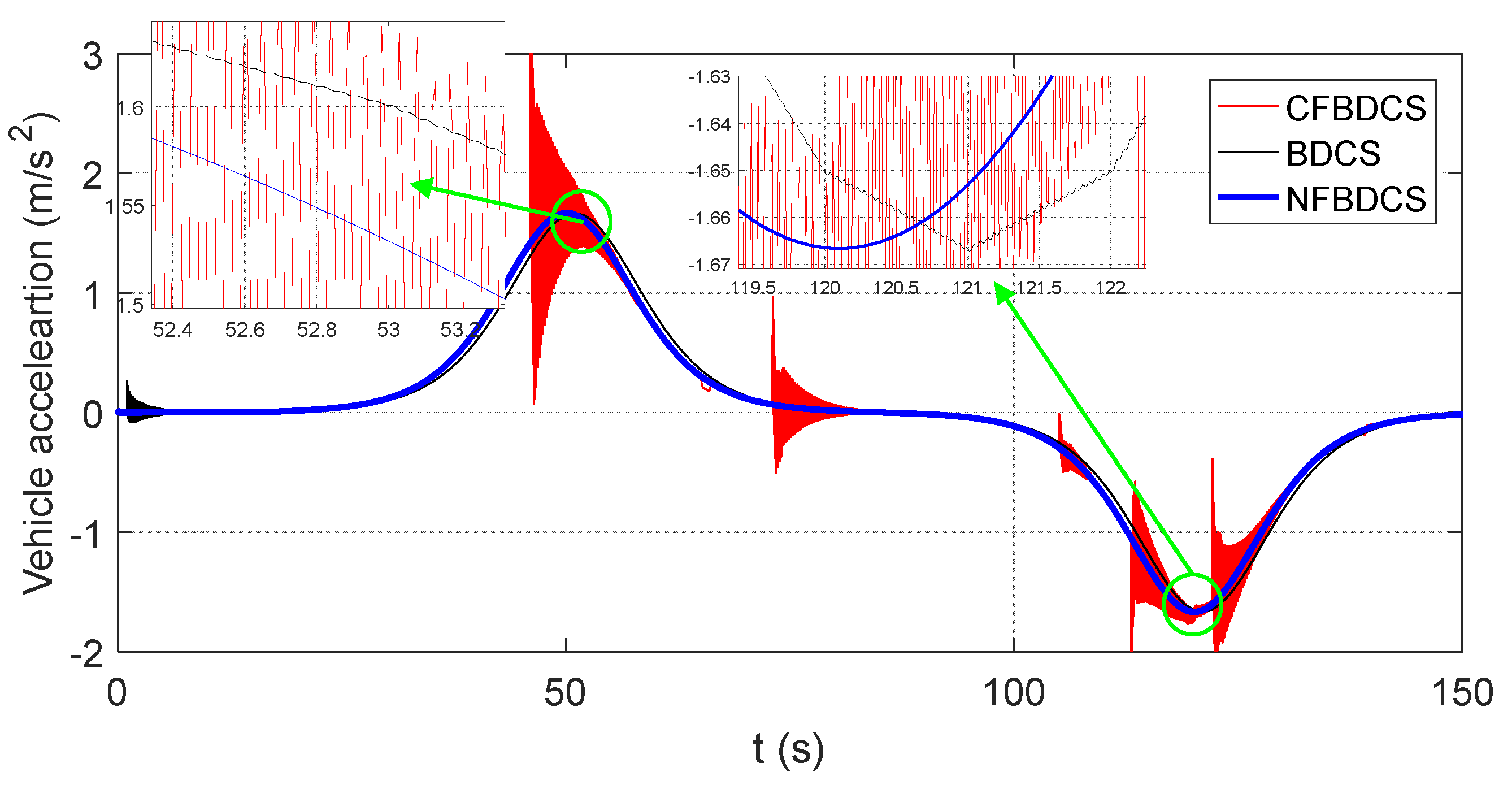
5.1. Dynamic Performance

This subsection compares the dynamic performance of the DMPAT under the three dynamic control strategies proposed in Section 4. A driving cycle shown in Figure 12 is designed to make the DMPAT experience all the three driving modes, so as to demonstrate the performance of three dynamic control strategies under different mode shifting conditions. Vehicle jerk is the main evaluation index of the dynamic performance.

To investigate the influence of the calling period of the EMS on the dynamic performance, two values Δt = 1 s and 0.1 s are considered. When Δt = 1 s, the corresponding driving modes changing with time is shown in Figure 13, in which all three driving modes occur in this driving cycle.

The torque of the two motors changing with time under the given driving cycle is shown in Figure 14. When the driving mode is changed, the torque of the two motors changes alternately, i.e., T₁ (or T₂) changes to zero from the current value while T₂ (or T₁) changes to the target value from zero. As a result, there is a large variation in the motor torque has for all the three dynamic control strategies. However, the motor torque under the BDCS and NFBDCS changes continuously, while the CFBDCS produces a step change of motor torque for most of the mode shifts. To show the detailed torque variation during the mode shifts, the amplified plots during some mode shifts are drawn in Figure 15, Figure 16, Figure 17 and Figure 18.

At the time of 105 s, the driving mode is changed from Mode 2 to Mode 1, shown in Figure 15. In this shifting process, T₂ changes from the initial values to zero, while T₁ changes from zero to the target torque. For the BDCS, the variation of both T₁ and T₂ follows the linear trajectories produced by the EMS. The torque variation tendency of the NFBDCS is similar to the BDCS, but the initial value of T₂ is different, and the trajectory of T₁ is controlled by the PI controller, which guarantees the total driving torque is smooth. For the CFBDCS, both T₁ and T₂ have a step change at the beginning of the mode shifting process (also see Figure 8), and then T₂ follows the same trajectory of the BDCS but T₁ is controlled by the PI controller. The step change of T₁ and T₂ produces a large jerk in the vehicle, shown in Figure 20.

At the time of 108 s, the driving mode is changed from Mode 1 to Mode 2, shown as Figure 16. The variation of T₁ and T₂ is in contrast to the case of Mode 2 changing to Mode 1, i.e., T₂ changes from zero to the target values while T₁ changes from the negative initial values to zero. For the BDCS, T₁ linearly increases from its initial value to zero in the period of 108 s and 109 s, while T₂ linearly changes from zero to its target value. For the NFBDCS, T₁ also linearly changes from its initial value to zero, while T₂ is controlled by the PI controller to compensate the variation of T₁. For the CFBDCS, there is a step change for T₁ and T₂ at the time of 108 s, which is induced by the switches in Figure 7. After 108 s, T₁ changes linearly while T₂ is directly controlled by the PI controller.

At time of 113 s, Mode 2 changes to Mode 1 & 2, shown in Figure 17. The mode shifting process from Mode 2 to Mode 1 & 2 is almost equivalent to the Mode 2 changing to Mode 1. The only difference is that the target value of T₂ is zero for Mode 1 while it is nonzero for Mode 1 & 2. Similarly, the process of Mode 1 & 2 changing to Mode 2 shown in Figure 18 is equivalent to that of Mode 1 changing to Mode 2, and the only difference is that the initial value of T₂ is nonzero for Mode 1 & 2 but it is zero for Mode 1. Both the BDCS and NFBDCS change T₁ and T₂ continuously, but the CFBDCS produces a step torque change, which produces a large vehicle jerk.

Figure 19 plots T₃ changing in the driving cycle, which demonstrates the total torque actuated on the vehicle. The BDCS and NFBDCS give a very smooth total driving torque to the vehicle, but the CFBDCS produces a large torque fluctuation at each time of mode shift, which is consistent with Figure 14.

The vehicle jerk under different dynamic control strategies is shown in Figure 20. Neglecting the large vehicle jerk in the initial dynamics balance stage, the CFBDCS still produces a very large vehicle jerk in most cases of mode shift, because its total driving torque has a step change when the driving mode changes. Both the BDCS and NFBDCS produce much less vehicle jerk since their total driving torque changes continuously. It is worth noting that there are many high-frequency fluctuations for the jerk of the BDCS but the jerk of the NFBDCS is quite smooth. This phenomenon is induced by the unsmooth change of driving torque of the BDCS (see Figure 6), since its torque is controlled by the EMS. On the contrary, the total driving torque of the NFBDCS is controlled by the PI controller, which makes the torque change smoothly, so as to produce much less vehicle jerk.

The dynamic performance of the three control strategies is also demonstrated by the vehicle acceleration, shown in Figure 21. The CFBDCS produces the large fluctuation of vehicle acceleration when the driving mode changes, but both the BDCS and NFBDCS have quite smooth vehicle acceleration during the mode shift. However, from the amplified plot it can be found that the BDCS still makes many vibrations, although the magnitude is quite small compared with the CFBDCS. The NFBDCS gives very smooth vehicle acceleration in the whole driving cycle, which makes the mode shift seamless.

The large vehicle jerk may be induced by the long calling period of the EMS, so a shorter calling period of EMS is considered in the following context, i.e., Δt = 0.1 s. The driving mode is shown in Figure 22, which has some difference to Figure 13. The vehicle jerk shown in Figure 23 indicates that the CFBDCS still produces the largest vehicle jerk during the mode shifting process, but it is a bit smaller than in the case of Δt = 1 s. The vehicle jerk of the BDCS becomes smoother than that of Δt = 1 s, so the shorter calling period of the EMS produces better performance for the BDCS. The NFBDCS is still the smoothest control method, which indicates that the NFBDCS is not influenced by the calling period of the EMS. It is worth noting that the calling period of the EMS cannot be extremely short, otherwise the EMS may not satisfy the requirements for real-time control.

The driving torque of the BDCS is absolutely based on the backward-facing dynamic model, so the accuracy of the parameters in the model determines its vehicle speed tracking performance. When all the parameters in the dynamic model are accurate, the BDCS can track the ideal vehicle speed. However, there are many unavoidable uncertain parameters in the system, e.g., the vehicle mass changes with the number of passengers. Considering the actual vehicle mass is larger than its normal value with 10% amplitude, the vehicle’s actual speed under the three control strategies is shown in Figure 24. It can be found that the BDCS cannot track the ideal vehicle speed, while the CFBDCS and NFBDCS have good tracking accuracy, because the CFBDCS and NFBDCS contain the PI controller which can adjust the driving torque based on the deviation of the vehicle’s actual speed and ideal speed. The vehicle speed tracking performance is quite important to develop automatic driving techniques. Of course, in human driving conditions the driver can adaptively adjust the accelerator pedal and brake pedal to track the expected vehicle speed. For example, when the vehicle is fully loaded, the experienced driver will press the pedals deeper than in empty-load conditions to make the vehicle achieve the same response speed. In this case, the PI controller is realized by the driver. If the PI controller has been included in the dynamic strategy, the driver would not need to adjust the pedals just because of a variation in the vehicle load.

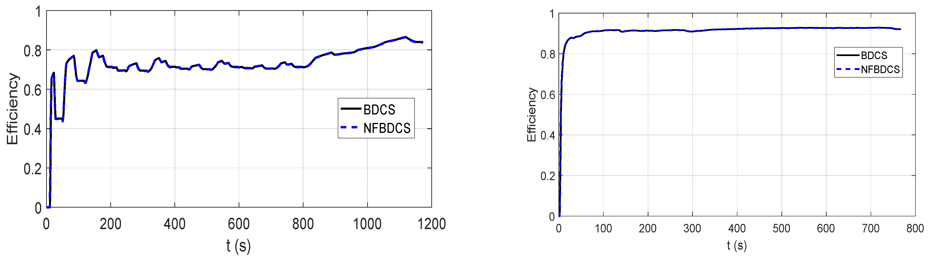
5.2. Energy Efficiency Analysis

Theoretically, the BDCS will produce the highest energy efficiency because it absolutely follows the backward torque provided by the EMS. When the NFBDCS is used, the actual driving torque is a little different to the backward torque produced by the EMS, so its energy efficiency may be lower. This subsection will compare the energy efficiency of the BDCS and NFBDCS based on the NEDC and HWFET driving cycles. The CFBDCS almost has the same efficiency as the NFBDCS, so it will not be compared here.

The energy efficiency for the two dynamic control strategies under the NEDC and HWFET driving cycles are shown in Figure 25. The results of both the NEDC and HWFET driving cycles demonstrate that there is almost no difference between the BDCS and NFBDCS in energy efficiency, so the energy efficiency is determined by the EMS rather than the dynamic control strategy.

6. Conclusions

This paper investigates the dynamic control strategies of a DMPAT for EVs. An optimized EMS is presented to select the driving mode and compute the driving torque for each motor by using the backward-facing dynamic model, and the detailed 5 DOF dynamic model of the powertrain is built to simulate the powertrain dynamic behavior more accurately. Three dynamic control strategies, i.e., BDCS, CFBDCS, and NFBDCS, are proposed to track the vehicle speed and realize the mode shift. The BDCS may produce large vehicle jerk when the calling period of EMS is relatively large, and it cannot track the vehicle speed when uncertain parameters exist in the system. The CFBDCS can track the vehicle speed accurately, but it produces large vehicle jerk during mode shift. The NFBDCS can track the vehicle speed accurately and produce a very small and smooth vehicle jerk during mode shift, and it is not affected by the calling period of EMS. Therefore, the NFBDCS is recommended to realize the seamless mode shift for a DMPAT.

The DMPAT does not contain any shifting actuator, e.g., clutch, brake, or synchronizer, so we only need to control the two driving motors to realize the mode shift, which has a lower control difficulty than other powertrains. It is worth noting that the motors always connect to the driving wheel in the DMPAT, so the average working efficiency of its motors is lower than that of powertrains equipped with shifting actuators. However, the DMPAT saves the parasitic energy loss induced by the shifting actuators, so a comprehensive energy efficiency analysis for the whole driving system should be further investigated.

References

1. Zhang, H.; Zhang, G.; Wang, J. H∞ Observer Design for LPV Systems with Uncertain Measurements on Scheduling Variables: Application to an Electric Ground Vehicle. IEEE/ASME Trans. Mechatron. 2016, 21, 1659–1670. [Google Scholar] [CrossRef]
2. Zhang, H.; Wang, J. Active Steering Actuator Fault Detection for An Automatically-steered Electric Ground Vehicle. IEEE Trans. Veh. Technol. 2017, 66, 3685–3702. [Google Scholar] [CrossRef]
3. Sorniotti, A.; Holdstock, T.; Pilone, G.L.; Viotto, F.; Bertolotto, S.; Everitt, M.; Barnes, R.J.; Stubbs, B.; Westby, M. Analysis and simulation of the gearshift methodology for a novel two-speed transmission system for electric powertrains with a central motor. Proc. Inst. Mech. Eng. Part D J. Automob. Eng. 2012, 226, 915–929. [Google Scholar] [CrossRef] [Green Version]
4. Husani, I. Electric and Hybrid Vehicles; CRC Press: Boca Raton, FL, USA, 2003. [Google Scholar]
5. Ehsani, M.; Gao, Y.; Emadi, A. Modern Electric, Hybrid Electric, and Fuel Cell Vehicles, 2nd ed.; CRC Press: Boca Raton, FL, USA, 2009. [Google Scholar]
6. Sorniotti, A.; Holdstock, T.; Everitt, M.; Fracchia, M.; Viotto, F.; Cavallino, C.; Bertolotto, S. A novel clutchless multiple-speed transmission for electric axles. Int. J. Powertrains 2013, 2, 103–131. [Google Scholar] [CrossRef] [Green Version]
7. Ren, Q.; Crolla, D.A.; Morris, A. Effect of Transmission Design on Electric Vehicle (EV) Performance. In Proceedings of the IEEE Vehicle Power and Propulsion Conference, Dearborn, MI, USA, 7–11 September 2009; pp. 1260–1265. [Google Scholar]
8. Hofman, T.; Steinbuch, M.; van Druten, R.M.; Serrarens, A.F.A. Rule-Based Energy Management Strategies for Hybrid Vehicle Drivetrains: A Fundamental Approach in Reducing Computation Time. IFAC Proc. Vol. 2006, 39, 740–745. [Google Scholar] [CrossRef] [Green Version]
9. Yu, C.-H.; Tseng, C.-Y. Research on gear-change control technology for the clutchless automatic–manual transmission of an electric vehicle. Proc. Inst. Mech. Eng. Part D J. Automob. Eng. 2013, 227, 1446–1458. [Google Scholar] [CrossRef]
10. Tseng, C.-Y.; Yu, C.-H. Advanced shifting control of synchronizer mechanisms for clutchless automatic manual transmission in an electric vehicle. Mech. Mach. Theory 2015, 84, 37–56. [Google Scholar] [CrossRef]
11. Ruan, J.; Walker, P.; Zhang, N. A comparative study energy consumption and costs of battery electric vehicle transmissions. Appl. Energy 2016, 165, 119–134. [Google Scholar] [CrossRef] [Green Version]
12. Shin, J.W.; Kim, J.O.; Choi, J.Y.; Oh, S.H. Design of 2-speed transmission for electric comercial vehicle. Int. J. Automot. Technol. 2014, 15, 145–150. [Google Scholar] [CrossRef]
13. Roozegar, M.; Angeles, J. The optimal gear-shifting for a multi-speed transmission system for electric vehicles. Mech. Mach. Theory 2017, 116, 1–13. [Google Scholar] [CrossRef]
14. Setiawan, Y.D.; Roozegar, M.; Zou, T.; Angeles, J. A Mathematical Model of Multispeed Transmissions in Electric Vehicles in the Presence of Gear Shifting. IEEE Trans. Veh. Technol. 2018, 67, 397–408. [Google Scholar] [CrossRef]
15. Holdstock, T.; Sorniotti, A.; Everitt, M.; Fracchia, M.; Bologna, S.; Bertolotto, S. Energy consumption analysis of a novel four-speed dual motor drivetrain for electric vehicles. In Proceedings of the IEEE Vehicle Power and Propulsion Conference, Seoul, Korea, 9–12 October 2012; pp. 295–300. [Google Scholar]
16. Hu, M.; Chen, S.; Zeng, J. Control Strategy for the Mode Switch of a Novel Dual-Motor Coupling Powertrain. IEEE Trans. Veh. Technol. 2018, 67, 2001–2013. [Google Scholar] [CrossRef]
17. Wu, J.; Liang, J.; Ruan, J.; Zhang, N.; Walker, P.D. Efficiency comparison of electric vehicles powertrains with dual motor and single motor input. Mech. Mach. Theory 2018, 128, 569–585. [Google Scholar] [CrossRef]
18. Hu, M.; Zeng, J.; Xu, S.; Fu, C.; Qin, D. Efficiency study of a dual-motor coupling EV powertrain. IEEE Trans. Veh. Technol. 2015, 64, 2252–2260. [Google Scholar] [CrossRef]
19. Hu, J.; Zu, G.; Jia, M.; Niu, X. Parameter matching and optimal energy management for a novel dual-motor multi-modes powertrain system. Mech. Syst. Signal Process. 2019, 116, 113–128. [Google Scholar] [CrossRef]
20. Hong, X.; Wu, J.; Zhang, N.; Wang, B.; Tian, Y. The dynamic and economic performance study of a new Simpson planetary gearset based dual motor powertrain for electric vehicles. Mech. Mach. Theory 2022, 167, 104579. [Google Scholar] [CrossRef]
21. Hong, X.; Wu, J.; Zhang, N.; Wang, B. Energy efficiency optimization of Simpson planetary gearset based dual-motor powertrains for electric vehicles. Energy 2022, 259, 124908. [Google Scholar] [CrossRef]
22. Wang, Z.; Zhou, J.; Rizzoni, G. A review of architectures and control strategies of dual-motor coupling powertrain systems for battery electric vehicles. Renew. Sustain. Energy Rev. 2022, 162, 112455. [Google Scholar] [CrossRef]
23. Yu, X.; Lin, C.; Zhao, M.; Yi, J.; Su, Y.; Liu, H. Optimal energy management strategy of a novel hybrid dual-motor transmission system for electric vehicles. Appl. Energy 2022, 321, 119395. [Google Scholar] [CrossRef]
24. Gao, B.; Liang, Q.; Xiang, Y.; Guo, L.; Chen, H. Gear ratio optimization and shift control of 2-speed I-AMT in electric vehicle. Mech. Syst. Signal Process. 2015, 50–51, 615–631. [Google Scholar] [CrossRef]
25. Liang, Q.; Gao, B.; Chen, H. Gear Shifting Control for Pure Electric Vehicle with Inverse-AMT. Appl. Mech. Mater. 2012, 190–191, 1286–1289. [Google Scholar] [CrossRef]
26. Hu, M.; Chen, L.; Wang, D.; Xu, Z.; Xu, P.; Qin, D.; Zhou, A. Modeling and characteristic study of the shifting engagement process in stepped transmission. Mech. Mach. Theory 2020, 151, 103912. [Google Scholar] [CrossRef]
27. Tian, Y.; Zhang, N.; Zhou, S.; Walker, P.D. Model and gear shifting control of a novel two-speed transmission for battery electric vehicles. Mech. Mach. Theory 2020, 152, 103902. [Google Scholar] [CrossRef]
28. Mo, W.; Wu, J.; Walker, P.D.; Zhang, N. Shift characteristics of a bilateral Harpoon-shift synchronizer for electric vehicles equipped with clutchless AMTs. Mech. Syst. Signal Process. 2021, 148, 107166. [Google Scholar] [CrossRef]
29. Roozegar, M.; Angeles, J. A two-phase control algorithm for gear-shifting in a novel multi-speed transmission for electric vehicles. Mech. Syst. Signal Process. 2018, 104, 145–154. [Google Scholar] [CrossRef]
30. Mousavi, M.S.R.; Pakniyat, A.; Wang, T.; Boulet, B. Seamless dual brake transmission for electric vehicles: Design, control and experiment. Mech. Mach. Theory 2015, 94, 96–118. [Google Scholar] [CrossRef]
31. Fang, S.; Song, J.; Song, H.; Tai, Y.; Li, F.; Sinh Nguyen, T. Design and control of a novel two-speed Uninterrupted Mechanical Transmission for electric vehicles. Mech. Syst. Signal Process. 2016, 75, 473–493. [Google Scholar] [CrossRef]
32. Tian, Y.; Ruan, J.; Zhang, N.; Wu, J.; Walker, P. Modelling and control of a novel two-speed transmission for electric vehicles. Mech. Mach. Theory 2018, 127, 13–32. [Google Scholar] [CrossRef]
33. Zhu, B.; Zhang, N.; Walker, P.; Zhan, W.; Zhou, X.; Ruan, J. Two-Speed DCT Electric Powertrain Shifting Control and Rig Testing. Adv. Mech. Eng. 2015, 5, 323917. [Google Scholar] [CrossRef]
34. Walker, P.; Zhu, B.; Zhang, N. Powertrain dynamics and control of a two speed dual clutch transmission for electric vehicles. Mech. Syst. Signal Process. 2017, 85, 1–15. [Google Scholar] [CrossRef]
35. Kim, S.; Oh, J.; Choi, S. Gear shift control of a dual-clutch transmission using optimal control allocation. Mech. Mach. Theory 2017, 113, 109–125. [Google Scholar] [CrossRef]
36. Li, G.; Görges, D. Optimal control of the gear shifting process for shift smoothness in dual-clutch transmissions. Mech. Syst. Signal Process. 2018, 103, 23–38. [Google Scholar] [CrossRef]
37. Liang, J.; Yang, H.; Wu, J.; Zhang, N.; Walker, P.D. Shifting and power sharing control of a novel dual input clutchless transmission for electric vehicles. Mech. Syst. Signal Process. 2018, 104, 725–743. [Google Scholar] [CrossRef]
38. Zhang, L.; Yang, L.; Guo, X.; Yuan, X. Stage-by-phase multivariable combination control for centralized and distributed drive modes switching of electric vehicles. Mech. Mach. Theory 2020, 147, 103752. [Google Scholar] [CrossRef]
39. Wu, J.; Zhang, N. Driving mode shift control for planetary gear based dual motor powertrain in electric vehicles. Mech. Mach. Theory 2021, 158, 104217. [Google Scholar] [CrossRef]
40. Wu, J.; Hong, X.; Feng, G.; Zhang, Y. Seamless mode shift control for a new Simpson planetary gearset based dual motor powertrain in electric vehicles. Mech. Mach. Theory 2022, 178, 105056. [Google Scholar] [CrossRef]
41. Zhao, Z.; Lei, D.; Chen, J.; Li, H. Optimal control of mode transition for four-wheel-drive hybrid electric vehicle with dry dual-clutch transmission. Mech. Syst. Signal Process. 2018, 105, 68–89. [Google Scholar] [CrossRef]
42. Wu, J.; Liang, J.; Ruan, J.; Zhang, N.; Walker, P.D. A robust energy management strategy for EVs with dual input power-split transmission. Mech. Syst. Signal Process. 2018, 111, 442–455. [Google Scholar] [CrossRef]
Figure 1. Layout of powertrain with DMPAT.
Actuators 11 00320 g001
Figure 2. (a) Power loss map of EM1, (b) Power loss map of EM2.
Actuators 11 00320 g002
Figure 3. 5 DOF dynamic model of transmission.
Actuators 11 00320 g003
Figure 4. (a) Torque distribution and driving modes under NEDC driving cycle. (b) Torque distribution and driving modes under NEDC driving cycle (amplified).
Actuators 11 00320 g004
Figure 5. Control scheme of BDCS.
Actuators 11 00320 g005
Figure 6. Schematic of mode shifting based on BDCS.
Actuators 11 00320 g006
Figure 7. Control scheme of CFBDCS.
Actuators 11 00320 g007
Figure 8. Schematic of mode shifting based on CFBDCS.
Actuators 11 00320 g008
Figure 9. Control scheme of NFBDCS.
Actuators 11 00320 g009
Figure 10. Schematic of mode shifting based on NFBDCS.
Actuators 11 00320 g010
Figure 11. Schematic of mode shifting of NFBDCS by adding the transition process.
Actuators 11 00320 g011
Figure 12. Designed vehicle speed profile.
Actuators 11 00320 g012
Figure 13. Vehicle driving mode with Δt = 1 s.
Actuators 11 00320 g013
Figure 14. Driving torque of EM1 and EM2 with Δt = 1 s.
Actuators 11 00320 g014
Figure 15. Torque profile from Mode 2 to Mode 1.
Actuators 11 00320 g015
Figure 16. Torque profile from Mode 1 to Mode 2.
Actuators 11 00320 g016
Figure 17. Torque profile from Mode 2 to Mode 1 & 2.
Actuators 11 00320 g017
Figure 18. Torque profile from Mode 1 & 2 to Mode 2.
Actuators 11 00320 g018
Figure 19. Total driving torque in the driving cycle.
Actuators 11 00320 g019
Figure 20. (a) Jerk of vehicle with Δt = 1 s, (b) Jerk of vehicle with Δt = 1 s (amplified).
Actuators 11 00320 g020
Figure 21. Vehicle acceleration with Δt = 1 s.
Actuators 11 00320 g021
Figure 22. Vehicle driving mode with Δt = 0.1 s.
Actuators 11 00320 g022
Figure 23. (a) Jerk of vehicle with Δt = 0.1 s, (b) Jerk of vehicle with Δt = 0.1 s (amplified).
Actuators 11 00320 g023
Figure 24. Vehicle speed tracking performance under uncertain conditions.
Actuators 11 00320 g024
Figure 25. Energy efficiency for NEDC (left) and HWFET (right) driving cycles.
Actuators 11 00320 g025