Predicting Multidimensional Poverty with Machine Learning Algorithms: An Open Data Source Approach Using Spatial Data

Abstract

This paper presents a methodology to estimate the multidimensional poverty index using spatial data at the street block level. The data used in this study were obtained from Open Street Maps and ESA’s land use cover, which are freely available sources of spatial information. The study employs five machine-learning algorithms, including Catboost, Lightboost, and Random Forest, to estimate the multidimensional poverty index with spatial granularity. The results indicate that these models achieve promising performance in predicting poverty levels in Medellín, Colombia. The results showed that the Random Forest algorithm achieved the highest performance, with an MAE of 0.07504. Furthermore, the spatial distribution of the multidimensional poverty estimate was highly correlated with the true values of the distribution. This work contributes to predicting multidimensional poverty by demonstrating the potential of machine learning algorithms to utilize accessible spatial data. By providing evidence of the feasibility of estimating poverty levels at a granular spatial level, this methodology offers a powerful tool for policymakers to make poverty social interventions with low-cost evidence. Furthermore, this study has important implications for poverty eradication efforts in developing countries, where access to reliable data remains challenging.

1. Introduction

The standard way of identifying poverty is based on income. That means that individuals with an income below a certain threshold are considered poor, and the number of people below that line determines the headcount ratio. However, this perspective is criticized by the theorists of the human development and capability approach (Alkire 2005; Nussbaum 2001; Sen 1985, 1999), widely arguing that income is not intrinsically essential but instrumentally significant, and the headcount income measurement is devoid of information on the reality of the poor (Sen 1985, 1992, 2017). Then, the income perspective is considered a resource or means that could be converted into valuable goals such as being educated, healthy, nourished, or even able to participate in society. Then, with the theory of capabilities, the understanding of poverty acquires a perspective centered on the human being, their beings, and doings. An important conclusion of the capabilities approach is to consider poverty and well-being as a problem of multiple dimensions in the sphere of the human being and not in elements distant from their beings or doings (functionings called in capability approach) (Nussbaum 2001; Sen 1999). In this sense, the multidimensional poverty index adopts the capability approach as the theoretical framework behind the measure (Alkire et al. 2015); the multidimensional poverty index approach uses indicators focused on identifying people’s deprivations to reach human dignity or well-being.

This perspective is part of the Sustainable Development Goals 2030 (SDGs) global agenda. To end poverty in all its forms and everywhere is the first aim. Moreover, the global multidimensional poverty index (MPI) is part of the indicators for monitoring progress in the first objective. In this case, poverty is understood as a result of simultaneous deprivation faced by the person or the household. Although the global MPI comprises three dimensions and ten variables (Alkire et al. 2020), the national poverty measures often have more dimensions and variables. In addition, it is common to see poverty measures with representativeness at the country or significant territory level. However, this is not the case for micro levels such as neighborhoods or blocks that may only be available with population censuses; these censuses are updated every ten years on average. Nevertheless, detailed and updated information on deprivation at the micro level is required for public policy to act with more precision and opportunity to eliminate poverty. Accordingly, it is important to have instruments to measure social indicators regularly, as poverty and well-being can change on a short-term basis. For example, the impacts of COVID-19 on multidimensional poverty are estimated through simulations, showing that 460 million more poor people would enter multidimensional poverty UNDP and OPHI (2021). In the Colombian case, the multidimensional poverty index (MPI) has five dimensions, with 15 variables in them (Angulo et al. 2016). The methodology approach follows the well-known MPI from Sabine Alkire and James Foster Alkire and Foster (2011); Alkire et al. (2015). The index identifies the headcount ratio and the gap between poor people; it has become an essential tool for social policymakers. However, the data available to calculate the index at the neighborhood level are in the census survey from 2018, which is made every ten years. Furthermore, there are places where the census data are not collected due to problematic access or problems of violence, mainly in rural areas. Furthermore, censuses are costly and time-consuming to implement. Hence, a low-cost method for estimating multidimensional poverty is a crucial tool for qualifying public policy decision-making.

Nevertheless, satellite earth observation data are crucial for understanding the socioeconomic measures from space, initially by the correlation between income and night-light images Blumenstock et al. (2015). However, after pointing the way with satellite images, new studies started going beyond the use of night-light images to predict socioeconomic conditions and wealth index indicators as a poverty proxy (Ayush et al. 2020; Engstrom et al. 2017; Jean et al. 2016; Lee and Braithwaite 2020; Steele et al. 2017). AI tools are being applied to predict and select variables that can explain poverty Hall et al. (2022); Usmanova et al. (2022). However, given the importance of the need to make progress in eradicating poverty everywhere, the multi-source geospatial data on multidimensional poverty mapping are considered an open area not fully explored Hu et al. (2022) as a source for both feature extraction and predictive variables.

Then, this study aims to use spatial features extracted from Open Street Maps and ESA’s land use cover to predict Colombians’ MPI in Medellín city. The focus is on understanding poverty at the block level due to its fine spatial granularity in order to bring poverty prediction closer to the realities of micro spatial units.

2. Related Works

Several studies have highlighted the relationship between social indicators and alternative data and applied machine learning and deep learning methodologies. The alternative data refer to sources other than surveys and census, mainly. There are countries or zones with no available data to predict social indicators of poverty or wealth, and when data are available, they need to be updated. In addition, the cost of updating is high because surveys covering large territories are required. These are the main arguments for using new artificial intelligence technologies to estimate social indicators as a proxy of poverty, an area of research that has been growing in recent years Hall et al. (2022); Usmanova et al. (2022). Following these concerns, one seminal work was made by (Blumenstock et al. 2015) using Call Detail Records (CDR) and the VIIRS-DNB satellite image data for predicting the wealth index in Rwanda from Demographic and Health Survey (DHS); the authors implemented deterministic finite automaton as feature extraction approach and linear methods with regularization approaches as the prediction algorithm. This perspective opened a research area where the satellite images, CDR, aerial images, and data geolocated are used to understand social indicators such as poverty, consumption, income, and wealth indices (Ayush et al. 2020; Engstrom et al. 2017; Jean et al. 2016; Lee and Braithwaite 2020; Niu et al. 2020; Pokhriyal and Jacques 2017; Pokhriyal et al. 2020; Steele et al. 2017; Watmough et al. 2019).

The methodological differences are presented in four aspects: the data source, the feature extraction methods, the prediction methods, and the target variable chosen. The models used the census or survey data geolocalized, which contains the ground truth variable; the primary source in several studies is the DHS survey that meets the two requirements: the household’s geolocation and the wealth index as a proxy of social condition (Blumenstock et al. 2015; Ledesma et al. 2020; Lee and Braithwaite 2020; Sheehan et al. 2019; Steele et al. 2017; Weidmann and Schutte 2017). Some works focus on census data as the main source (Engstrom et al. 2017; Pandey et al. 2018; Pokhriyal and Jacques 2017; Pokhriyal et al. 2020), while others focus on local or national surveys (Ayush et al. 2020; Gebru et al. 2017; Steele et al. 2017; Watmough et al. 2019). In addition to using satellite imagery, some studies combine data from different sources, such as Wikipedia geolocated articles (Sheehan et al. 2019), the settlement data from the United Nations (Lee and Braithwaite 2020), the points of interest from OpenStreetMaps (Hu et al. 2022; Ledesma et al. 2020; Lee and Braithwaite 2020), Google street view images (Gebru et al. 2017), counting of users from Facebook (Ledesma et al. 2020), aerial images (Pokhriyal et al. 2020), indicators from open platforms Niu et al. (2020), street level images Suel et al. (2021), and call detail records (Blumenstock et al. 2015; Moya-Gómez et al. 2021; Pokhriyal and Jacques 2017; Pokhriyal et al. 2020; Steele et al. 2017). The combination of data sources has demonstrated promising results for multidimensional poverty estimation (Pokhriyal and Jacques 2017; Pokhriyal et al. 2020).

Regarding feature extraction, new approaches have embraced the convolutional neural network (CNN) because the main data source has been satellite images, which are combined with geolocated data surveys and different prediction methods. Some applications, using CNN as a feature extraction method and linear regression methods as a prediction approach, estimate the income and consumption index in some African countries (Engstrom et al. 2017; Jean et al. 2016). Others estimate social demographic indicators in the United States through ridge regression (Gebru et al. 2017). Keeping the CNN as a feature extraction algorithm, the applications broaden the perspective of prediction methods and include tree-based and boosting methods for predicting the wealth index from the DHS survey (Lee and Braithwaite 2020) and consumer expenditure index (Ayush et al. 2020). Furthermore, a multitask fully connected neural network has been implemented for predicting the roof type, source of lighting, and the source of drinking water for rural villages in India (Pandey et al. 2018), and in a simple fully connected network for predicting the international wealth index (Sheehan et al. 2019). In addition, there are works using extraction methods such as geospatial environmental models (Watmough et al. 2019), counting methods based on descriptive statistics or linear transformations (Ledesma et al. 2020; Niu et al. 2020; Weidmann and Schutte 2017), gaussian process regression (Pokhriyal et al. 2020), document representation (Sheehan et al. 2019), and non-spatial generalized linear models (Steele et al. 2017).

To predict methods, there is a tendency to use multiple prediction algorithms in order to compare performances; one remarkable work uses several algorithms such as Random Forest, Gradient Boosting Machines, linear models with regularization, deep learning models, and new strategies such as the Stacked Learning Process (Pokhriyal et al. 2020). However, studies that seek to advance the explanatory capacity of the models show that Random Forest is the best-performing algorithm Hu et al. (2022); Liu et al. (2021); Niu et al. (2020); Puttanapong et al. (2022); Usmanova et al. (2022); in fact, the algorithm is considered one of the best options for poverty prediction Sohnesen and Stender (2017).

Previous research in this field has predominantly focused on estimating income, wealth, and general indicators as a proxy of poverty, with comparatively less attention devoted to examining poverty from a multidimensional perspective. Based on the literature reviewed, few studies use different inequality and multidimensional poverty indices as response variables (Pokhriyal and Jacques 2017; Pokhriyal et al. 2020; Puttanapong et al. 2022). In general, estimating an MPI through spatial data has received limited attention, even when the first Sustainable Development Goal is to eradicate extreme poverty in all its forms everywhere, and even the world observed that the COVID-19 pandemic increased poverty rates Sachs et al. (2021). However, it is essential to mention that the area of poverty prediction research using artificial intelligence algorithms is progressing rapidly Hall et al. (2022); Usmanova et al. (2022).

In this regard, following the same intention as the studies above, in Colombia, a recent study by the National Department of Statistics (DANE by the Spanish acronym) conducted three experiments for predicting Colombia’s MPI. They used the mentioned metric at a neighbor level as the response variable. They use convolutional neural networks for feature extraction, followed by an estimation process with machine learning algorithms. The experiments start from a baseline, where they estimate poverty with classical covariates in the last census of 2018. The details of the experiments they performed were shared in their repository1 and can be outlined as follows:

• They use census covariates as predictors and the Principal Component Analysis (PCA) as a multidimensional reduction technique, choosing five components. They reported that their MPI has 0 and 1 values, which they excluded for the first experiment. Gradient Boosting tree regression and Random Forest were the methods. The best performance result was using the Gradient Boosting algorithm (r-squared equal to 0.6789, and RMSE equal to 0.7818);
• In the second experiment, they used the same variables as the first one, but this time they included the 0 and 1 MPI values. The best result was using the Gradient Boosting algorithm; the R-squared was equal to 0.6537 and the RMSE equal to 1.1898; meanwhile, with the second-best algorithm, they achieved an R-squared of 62.81% and an RMSE of 1.233;
• In The third experiment, they used sentinel-2 images as input features. They used Resnet34 as a pre-trained model to transfer knowledge and fine-tune the data. They applied data augmentation, rotations of 90 degrees on the horizontal and vertical axis were performed, and image contrast was performed. They extracted 512 covariates from the neural network (the weights). After the future extraction, they applied PCA to obtain five components, which they interpolated with the natural neighbor’s method at the block level. They estimated the MPI using approach 1 (A1), which includes the 0 and 1 MPI values, and approach 2 (A2), which excludes the 0 and 1 values. The best result reported reached an RMSE equal to 0.9067 and an R-squared equal to 0.5757 using a Random Forest as a classifier and following the A2 approach.

Dane’s methodology is based on a deep learning process using hard-to-access data and algorithms that require considerable computational power. In the proposal, open-access data are utilized alongside less complex pre-processing and easy-to-use machine learning algorithms, which enable advancement in the interpretability of estimation models. That is an aspect that is stated in the literature as a challenge in the models that use IA tools for poverty estimation Hall et al. (2022).

Contributions of This Study

• Propose an accessible data source to estimate multidimensional poverty at a high level of granularity;
• Apply machine learning methods on spatial features to estimate multidimensional poverty at the street block level.

3. Materials and Methods

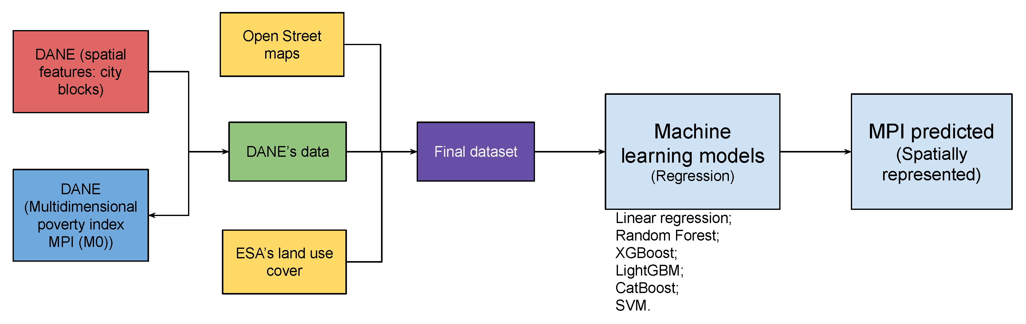
The general methodology is presented in Figure 1. We map the geolocated MPI ($M_0$) (Alkire and Foster 2011). The $M_0$ index is the outcome of interest predicted with spatial data extracted from the Open Street Maps, DANE, and ESA. The data extracted for the estimation are freely available and easily accessible. The input database comprises geolocated variables, integrated with MPI data by blocks. We use the following models for prediction: linear regression, support vector machine, Random Forest, LightGBM, XGBoost, and Catboost. In order to check the prediction patterns, the spatial representation of the forecast is compared against the ground truth values.

3.1. Area of Interest

The area of interest corresponds to the urban area of Medellín, Colombia. Medellín is the capital of Antioquia’s department and one of the most prosperous cities in the country. This area had 3,933,652 inhabitants in 2018 and 380.64 square kilometers. Furthermore, it has a population density of 10,351 persons per square kilometer. The administrative spatial units in the urban area are communes (16) and neighborhoods (243). Medellín is a city with social segregation dynamics marked by spatial patterns; the excluded and vulnerable people are located in peripheral areas in the north of the city, mainly Moya-Gómez et al. (2021); Santa et al. (2019).

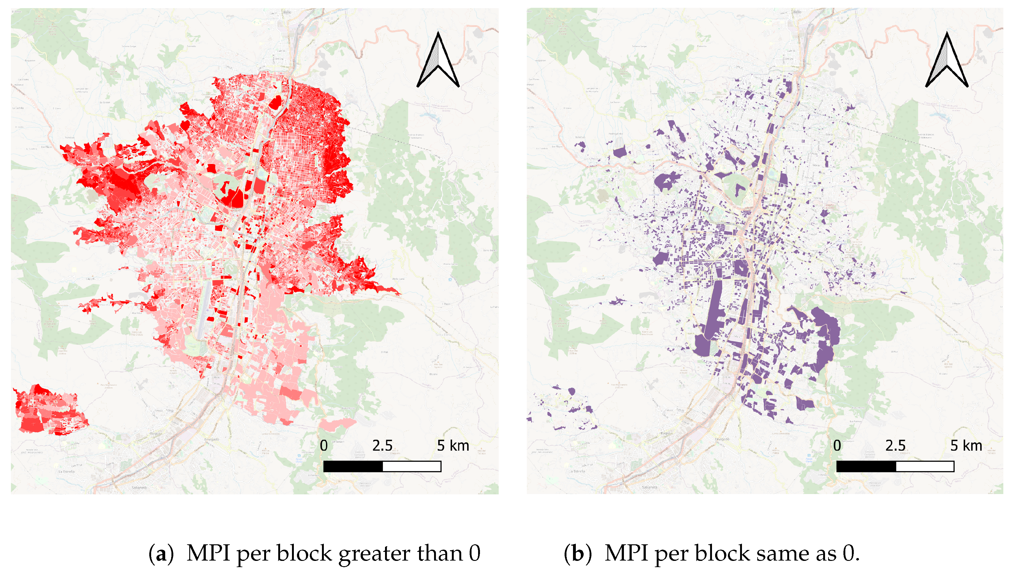
The distribution of the MPI in Medellín, Colombia, is introduced in Figure 2a,b. The peripheral areas have the highest values, represented by red, mainly in the northeast, contrasting with the southeast, where the MPI is low.

This representation is in line with the Spatial distribution of quality of life in the city, which evidences that the Poblado commune (The southeast zone) is the territory with the highest quality of life in the city, and the Popular commune (northeast) with the lowest. A result confirmed by studies that improve the scale of analysis by calculating and spatializing an alternative quality of life indicator to the one used by the city, but using the same quality of life survey Sepúlveda Murillo et al. (2019). The spatial distribution of the MPI is represented by polygons. Some of these polygons do not have an estimated MPI because they correspond to non-residential spaces, such as universities, business buildings, cultural or sports facilities, and commercial areas; also, there are errors in the census data related to a lack of information to estimate the MPI in some blocks; Figure 2b represent the areas where the MPI is same as zero.

3.2. Data

We implemented the combination of different data sources with attention to making the data freely accessible and easy to obtain. Combining different data sources provided improved predictive power and lower errors in estimating poverty than using these separately (Pokhriyal and Jacques 2017; Pokhriyal et al. 2020). The dataset used to estimate multidimensional poverty was sourced from Colombia’s 2018 population census. The country’s administrative department of statistics is responsible for computing the MPI per block using this census. It is precisely this index that serves as the response variable of the estimated models in the current study. The data from Open Street maps were downloaded in May 2022 from Planet OSM2. The following section expounds upon the source and the type of data employed, with particular emphasis on their salient features and characteristics.

3.2.1. National Department of Statistics (DANE)

The DANE calculates the MPI by blocks from Colombia’s 2018 census. This information is available in Dane’s geoportal3. Each block is defined by the administrative department and has its own identifier. For this study, the MPI by blocks is defined as the response variable.

The MPI in Colombia follows the Alkire–Foster methodology Alkire and Foster (2011). It has five dimensions and 15 indicators; when a household is deprived in at least 33% of the indicators, it is considered multidimensional poor (Angulo et al. 2016). The methodology has three leading outcome indicators: the headcount ratio of multidimensional poverty H, the average intensity of multidimensional poverty A, and the adjusted headcount ratio $M_0$. The $M_0$ is the product of the H an A ($M_0=HXA$), which reflects the incidence of poverty and the intensity, and captures the joint distribution of deprivations (Alkire et al. 2015). This study uses the $M_0$ as an MPI.

3.2.2. OpenStreetMaps (OSM)

OpenStreetMap is a collaborative project that collectively generates spatial databases. The current study posits that the distance to the reference points under consideration is contingent upon the hypothesis that the built environments of these locations are associated with the prevailing socioeconomic conditions Hu et al. (2016); Li and Liu (2019); Niu et al. (2020); Xi et al. (2022); Ye et al. 2011, 2019. These points of interest, as identified in this study, are envisaged to serve as reliable indicators of the spatial distribution of socioeconomic status. The geographical datasets for the region of interest were downloaded from OSM’s website. The features gathered were related to distance to police stations, hospitals, schools, universities, churches, airports, banks, train stations, and bus stops.

3.2.3. European Space Agency (ESA)

Data from the ESA related to land use were downloaded from the European Space Agency website. The data used for this analysis correspond to the 2020 land use cover with a 10 × 10 m resolution. These data were overlaid and compared with the OSM datasets. Later, a 10 × 10 m grid was used to calculate the number of hectares per cell, considering the different types of land uses.

3.3. Methods

We implemented several machine learning algorithms for estimating the MPI. We tested regularized linear regression (LR), support vector machine (SVM), Random Forest (RF), eXtreme Gradient Boosting (XGBoost), Light Gradient Boosting (LightGMB), and Category Boosting (CatBoost) algorithms.

3.3.1. Linear Regression

The linear regression is based on the least squares method to fit models with numeric outcomes. We applied the lasso shrinkage method to reduce the prediction error. Following the (Hastie et al. 2017) notation, the lasso estimate is defined by the equation:

$$\begin{array}{cc}\hfill {\widehat{\beta }}^{\mathrm{lasso}}=& \underset{\beta }{argmin}\sum _{i=1}^N{\left(y_i-{\beta }_0-\sum _{j=1}^p{x}_{ij}{\beta }_j\right)}^2\hfill \\ \hfill & \mathrm{subject}\mathrm{to}\sum _{j=1}^p\left|{\beta }_j\right|\le t\hfill \end{array}$$

(1)

The equivalent Lagrangian form shows the lasso penalty ${\sum }_1^p\left|{\beta }_j\right|$. That constraint makes the solutions nonlinear in the $y_i$ (Hastie et al. 2017). The lasso performs kin of continuous subset selection because some coefficients could be exactly zero when t is small.

$${\widehat{\beta }}^{\mathrm{lasso}}=\underset{\beta }{argmin}\left\{\frac{1}{2}\sum _{i=1}^N{\left(y_i-{\beta }_0-\sum _{j=1}^p{x}_{ij}{\beta }_j\right)}^2+\lambda \sum _{j=1}^p\left|{\beta }_j\right|\right\}.$$

(2)

3.3.2. Support Vector Regression Machine

The support vector machine regression is inspired by the classification version, which constructs an optimal separating hyperplane between two classes. It can be adapted for regression with a quantitative response. Where the linear regression model is given by

$$f\left(x\right)=x^T\beta +{\beta }_0$$

(3)

Then, a minimization function was considered to estimate B, where

$$H\left(\beta ,{\beta }_0\right)=\sum _{i=1}^{N}V\left(y_i-f\left(x_i\right)\right)+\frac{\lambda }{2}{\parallel \beta \parallel }^2$$

(4)

The quantity $\lambda$ is a regularization parameter. The “e-insensitive” error function for the support vector regression machine is defined by

$$V_{ϵ}\left(r\right)=\left\{\begin{array}{cc}0\hfill & \mathrm{if}\left|r\right|<ϵ\hfill \\ \left|r\right|-ϵ,\hfill & \mathrm{otherwise}\hfill \end{array}\right.$$

(5)

The solutions to the minimization problem

$$\begin{array}{cc}\hfill \widehat{\beta }& =\sum _{i=1}^N\left({\widehat{\alpha }}_i^{*}-{\widehat{\alpha }}_i\right)x_i\hfill \\ \hfill \widehat{f}\left(x\right)& =\sum _{i=1}^N\left({\widehat{\alpha }}_i^{*}-{\widehat{\alpha }}_i\right)〈x,x_i〉+{\beta }_0\hfill \end{array}$$

(6)

where ${\widehat{\alpha }}_i$ and ${\widehat{\alpha }}_i^{*}$ are positive and solve the quadratic programming problem. The solution depends on the inner products, which are defined by the kernel space selected (Hastie et al. 2017).

$$\underset{{\alpha }_i,{\alpha }_i^{*}}{min}ϵ\sum _{i=1}^N\left({\alpha }_i^{*}+{\alpha }_i\right)-\sum _{i=1}^N{y}_i\left({\alpha }_i^{*}-{\alpha }_i\right)+\frac{1}{2}\sum _{i,i^{\prime }=1}^N\left({\alpha }_i^{*}-{\alpha }_i\right)\left({\alpha }_{i^{\prime }}^{*}-{\alpha }_{i^{\prime }}\right)〈x_i,x_{i^{\prime }}〉$$

(7)

Subject to the constraints

$$\begin{array}{c}0\le {\alpha }_i,{\alpha }_i^{*}\le 1/\lambda \\ {\displaystyle \sum _{i=1}^N}\left({\alpha }_i^{*}-{\alpha }_i\right)=0\\ {\alpha }_i{\alpha }_i^{*}=0\end{array}$$

(8)

3.3.3. Random Forest

It is one of the most widely used algorithms for classification tasks due to its high performance and the identification of explanatory variables (Schonlau and Zou 2020). The algorithm is an ensemble method that uses different decision trees built on repeated training samples taken from the same training dataset (bootstrap method); this allows us to reduce the variance by calculating the average value of the set of models estimated independently. Using different predictor variables for tree construction generates randomness and reduces variance compared to classical tree-based methods (Hastie et al. 2017). The algorithm is robust to outliers and noise, and it is also faster than Adaboost and Bagging. Moreover, internal estimation of error, correlation, and variables of importance can be obtained (Breiman 2001). The Random Forest algorithm identifies nonlinear relations between explanatory and dependent variables, and it is one of the best-suited machine learning algorithms for variable importance assessment. The algorithm has fewer tuning hyperparameters compared to other machine learning methods.

3.3.4. eXtreme Gradient Boosting XGBoost

XGBoost stands for extreme gradient boost model algorithm and is useful for classification or regression. This method is one of the best-supervised learning algorithms. The loss function is included in the objective function and the regularization, while the model compares the results between real and predicted values (Jangaraj et al. 2021).

This model has achieved the state of the art in several contests held worldwide. Another important aspect of this algorithm is the scalability in all scenarios due to the algorithmic optimizations. It exploits out-of-core computation, allowing researchers to run the model on a desktop.

3.3.5. Light Gradient Boosting Machine LightGBM

The Light Gradient Boosting Machine (LightGBM) is one of the most important algorithms useful for classification or regression models. This algorithm was published in 2017, and it splits the node that maximizes the drop in the loss function. It introduces “exclusive feature bundling,” which collapses sparse descriptors into a particular feature. Another characteristic is that the method reduces the computational time and memory usage [Light Gradient Boosting Machine as a Regression Method for Quantitative Structure-Activity Relationships]. This algorithm becomes much faster than XGBoost while reducing the memory too. Microsoft distributed and maintained the entire code, which can be found on the website4.

3.3.6. CatBoost

Catboost is open-source software. It is based on a gradient-boosted decision tree useful for classification or regression purposes (Ibrahim et al. 2020; Prokhorenkova et al. 2019).

Having a dataset with the following:

$$D={\left\{\left(x_j,y_j\right)\right\}}_{j=1,\dots ,m}$$

(9)

where $X_j=(x_j^1,x_j^2,...,x_j^n)$ corresponds to a vector of n features and a response variable $y_j$. The response variable, in this case, could be numerical but binary or encoded, allowing for greater flexibility in modeling. The objective is to train a function H: $R^n\to R$ that maximizes the expected loss.

$$L\left(H\right):=EL(y,H(X\left)\right)$$

(10)

where $L\left(H\right)$ is a smooth loss function. The function $H^t$ is obtained through additive process in the following way: $H^t=H^{t-1}+\alpha g^t$, where $\alpha$ is a step function, and the function $g^t$ is a base predictor. Furthermore, it is defined as follows:

$$g^t={argmin}_{g\in G}L\left(H^{t-1}+g\right)={argmin}_{g\in G}EL\left(y,H^{t-1}\left(X\right)+g\left(X\right)\right)$$

(11)

3.4. Data Preparation and Estimation

A normalization process was performed to variable MPI using spatial blocks as units of measurement. Where the MPI was calculated as 0, greater than 100, or NULL, were dropped from the analysis. These values are considered errors or no MPI information.

Using the OSM data, the distance from the centroid of each street block to places such as airways, banks, churches, transportation, education, hospital, and police stations is calculated. Furthermore, the binning process is used as a part of feature engineering where the distances are in the following intervals: 0:100 m, 1:500 m, 2:1 km, 3:5 km, 4:more than 5 km.

The urban blocks in Colombia have a length between 80 and 100 m5. Around 400 to 500 m bus stations are found in Colombia’s urban areas, such as Bogotá. Sugiyama, et al. (Sugiyama et al. 2019). found that the median distance varies depending on the destination types, for example, around 600 m to public transit; for shops, other services, and utilitarian destinations between 800 m and 1.2 km; 2.3 km to natural features. Daniels and Mulley (Daniels and Mulley 2013) also noticed that most walking distances are less than 2 km. More than 10% of their sample takes trips less than 100 m. Moreover, more than 50% of the total sample is concentrated on walking trips of less than 600 m. However, the suburbs near Bogotá or Medellin have fewer resources than the urban areas, so pedestrians need to take transportation to reach special services (1 km–5 km), such as governmental offices, for instance, the case of Suba at the north-west of the capital city. Moreover, travel more than 5 km to reach places for recreation and rest, such as Zipaquirá salt mines in the North of Bogotá. Therefore, the previous buffers were defined based on previous studies and the geographical features of the main areas.

In addition to the variables from spatial data, a nominal variable is constructed to automatically separate the hillside zones from the middle and downtown areas. This is performed by looking for a variable that captures some of the spatial differences of the MPI index observed in the exploratory spatial distributions.

We implemented two optimization processes. The first one used cross-validation with ten folds and ten repeats on a search grid of 30 combinations of the different hyperparameters of the estimated algorithms; this was a soft estimation. The second one was performed by using ten folds and five repeats in the case of the random forest on a grid of 100 combinations of the different hyperparameters.

The database was split in two, 80% for training and 20% for testing; the Mean Absolute Error (MAE) was chosen to measure model comparison to select the best model in the training stage.

3.5. Software

QGIS 3.22.3 was used to perform spatial operations and visualization. Python 3.9 was used to unify DANE’s information and gather and merge spatial datasets from multiple sources. Furthermore, R x64 4.1.2 created the pipelines for the machine learning models.

4. Results

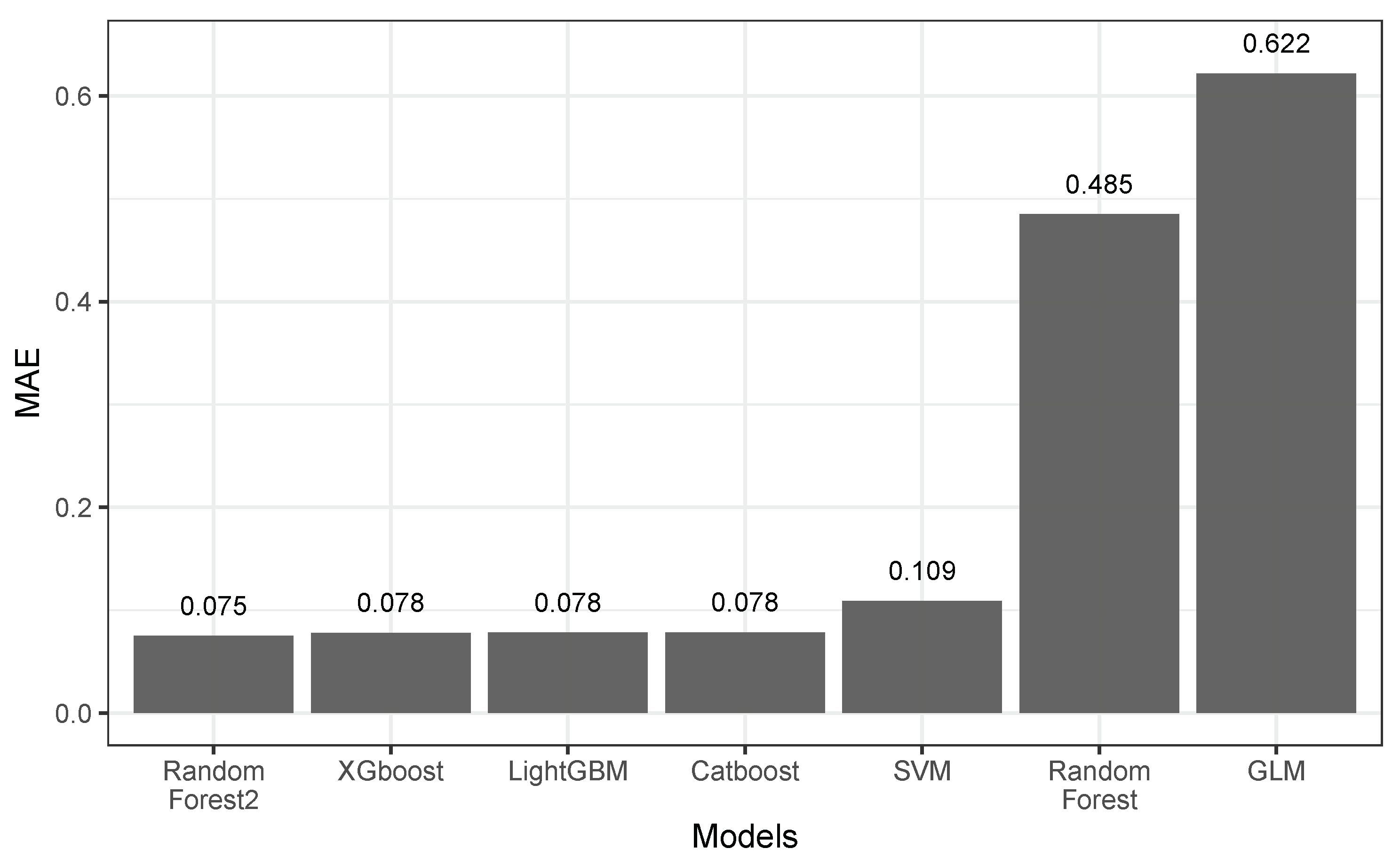
In the case of the General Linear Model (GLM), the linear regression yielded an MAE of 0.622, which serves as a baseline for evaluating the performance of the higher complexity algorithms implemented. Owing to the need for comprehensive multidimensional poverty estimation studies in the examined territory, the base model is the reference for comparative purposes. In the absence of previous studies, the base model enables evaluation of the effectiveness of the proposed methodology and establishes a solid foundation for assessing the predictive capabilities of subsequent models.

In this sense, the best models with similar MAE performance were Random Forest2 (0.07504), XGBoost (0.07804), LightGBM (0.07824), and CatBoost (0.07846) (Figure 3). It is essential to highlight that the Random Forest model with a higher MAE value (0.485) showed a spatial prediction pattern similar to the ground truth values. The difference between the two random forest models is due to the depth of the optimization process: the model with better performance was optimized with more iterations (hard optimization), while the model with high MAE was optimized with fewer iterations (soft optimization). Compared to the baseline, the results present consistent performance close to the ground truth values.

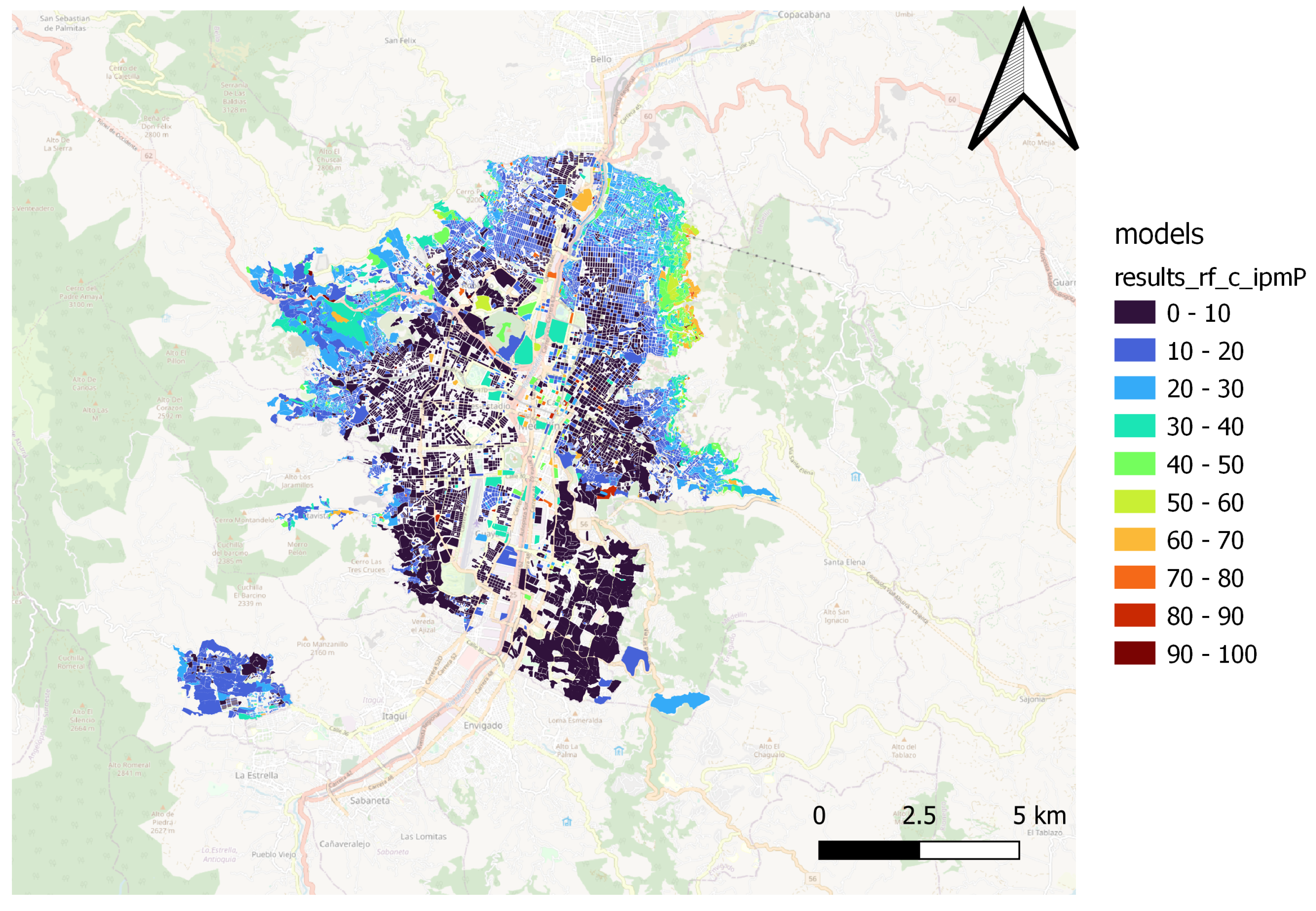
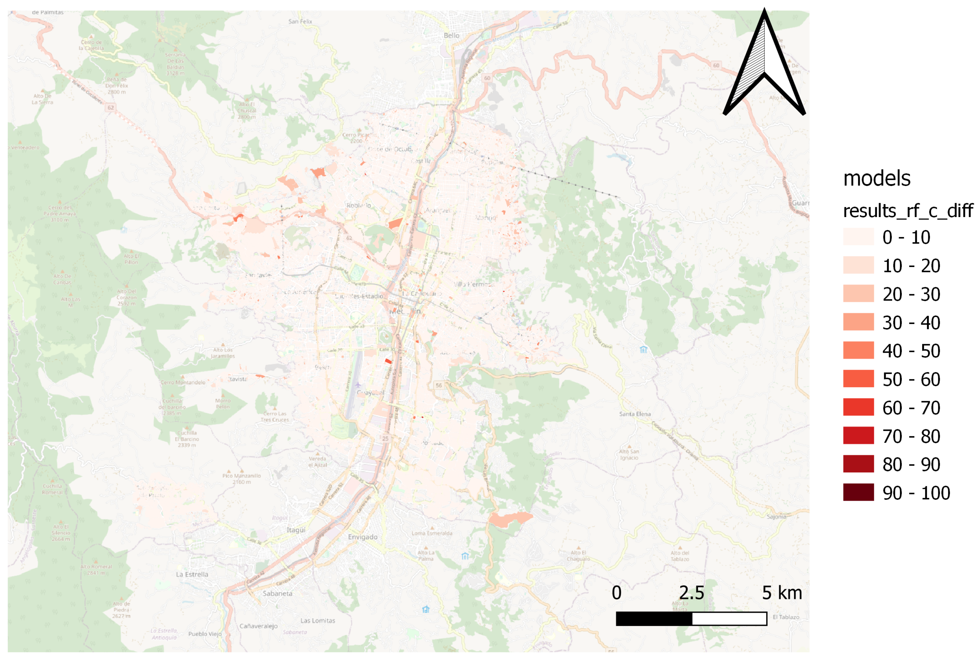
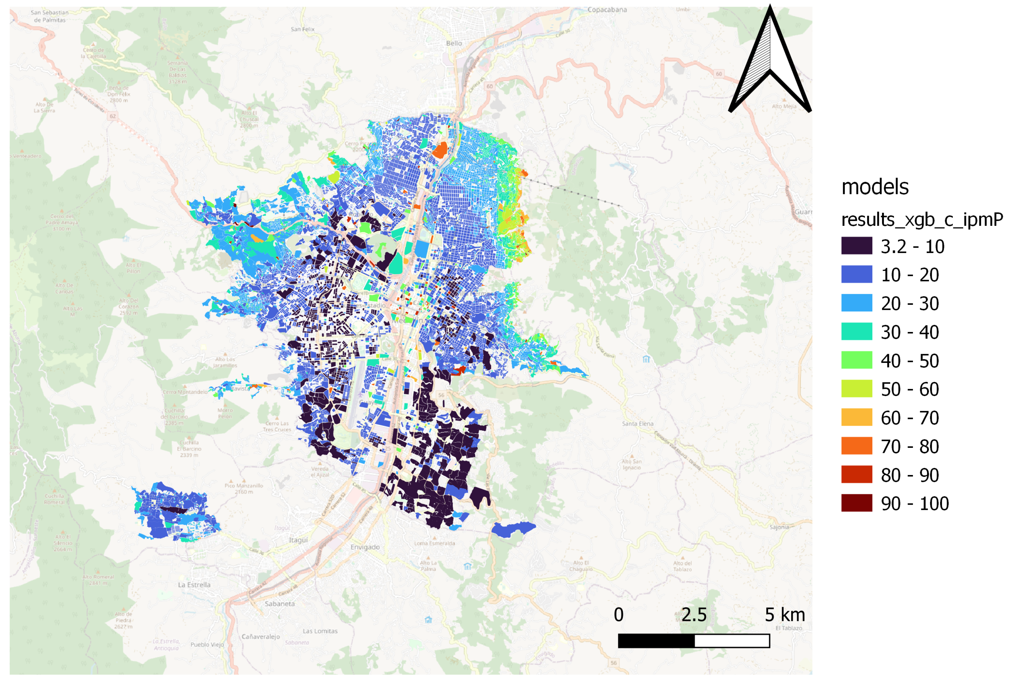
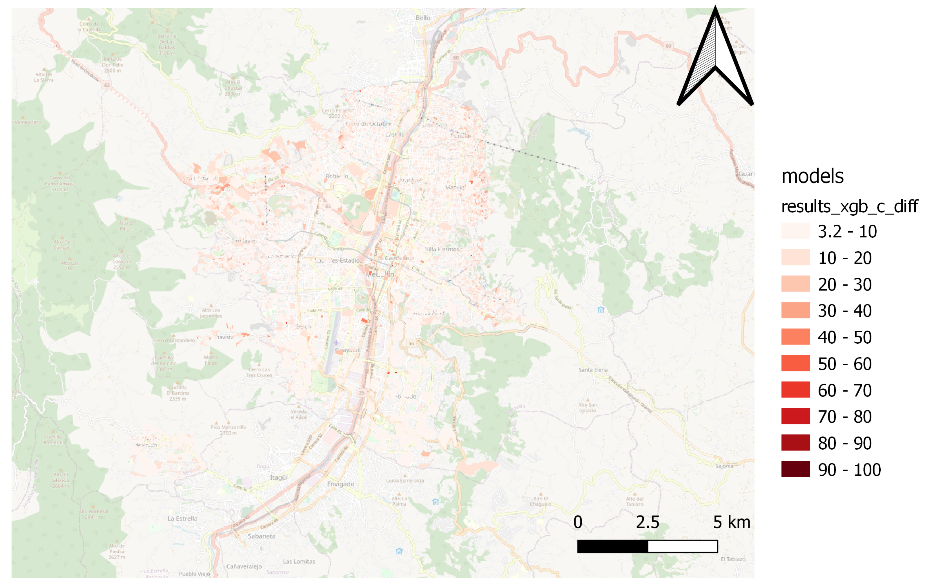
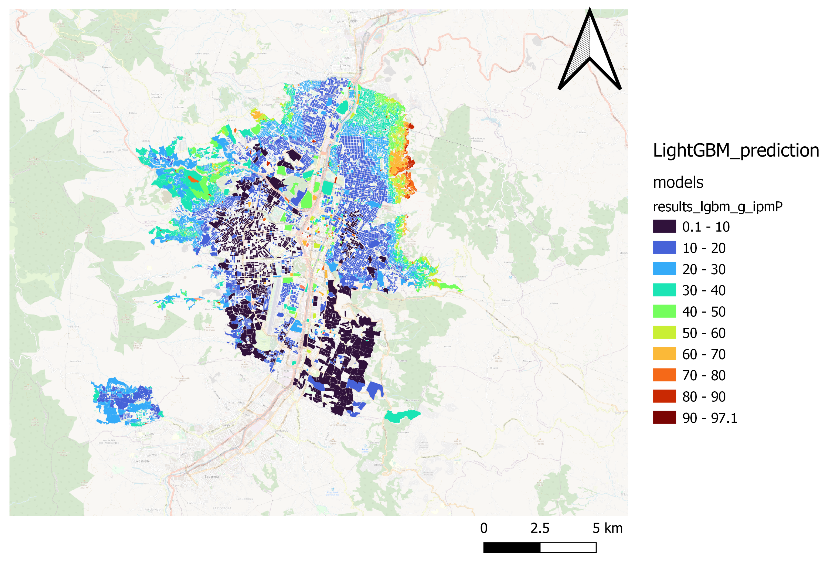
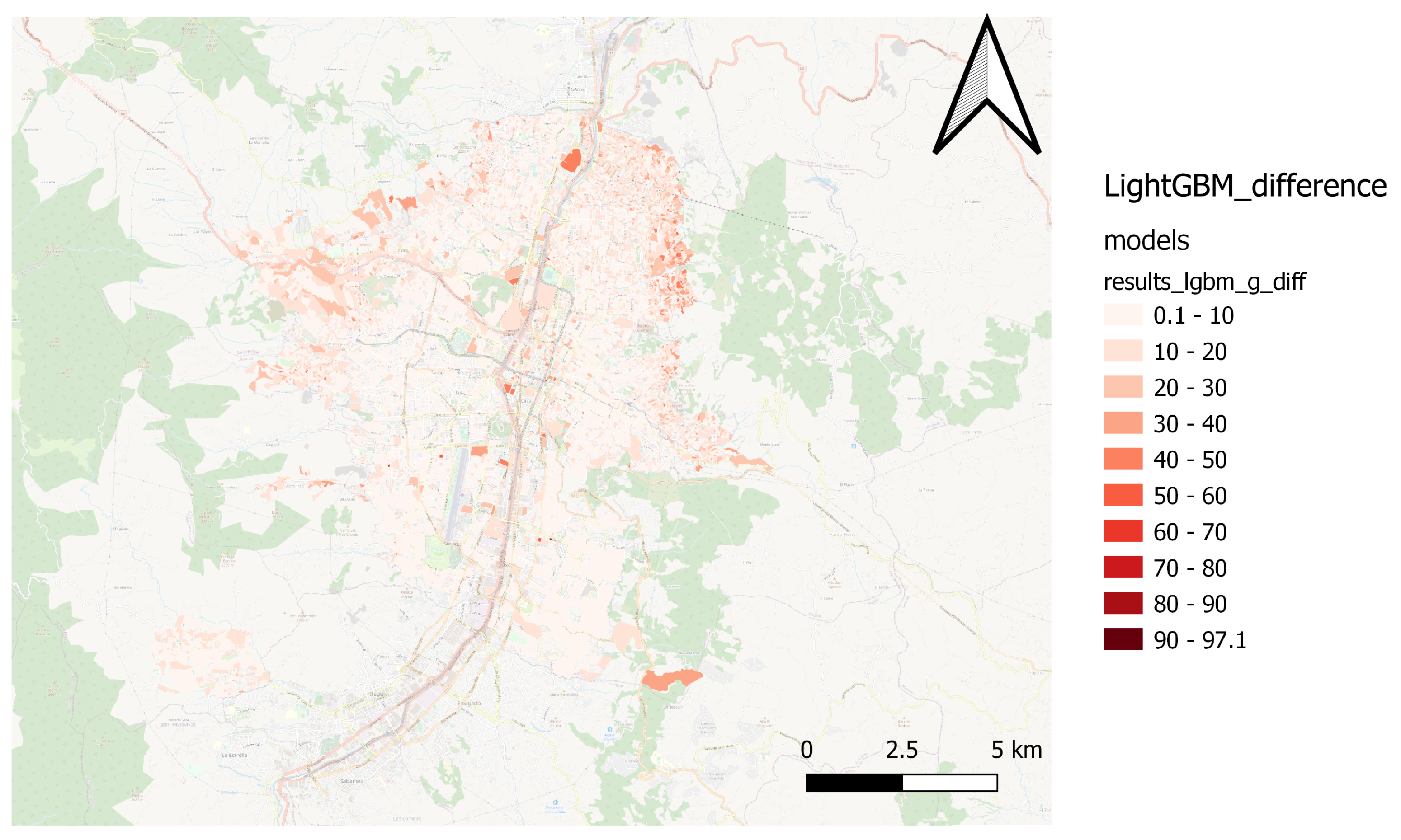
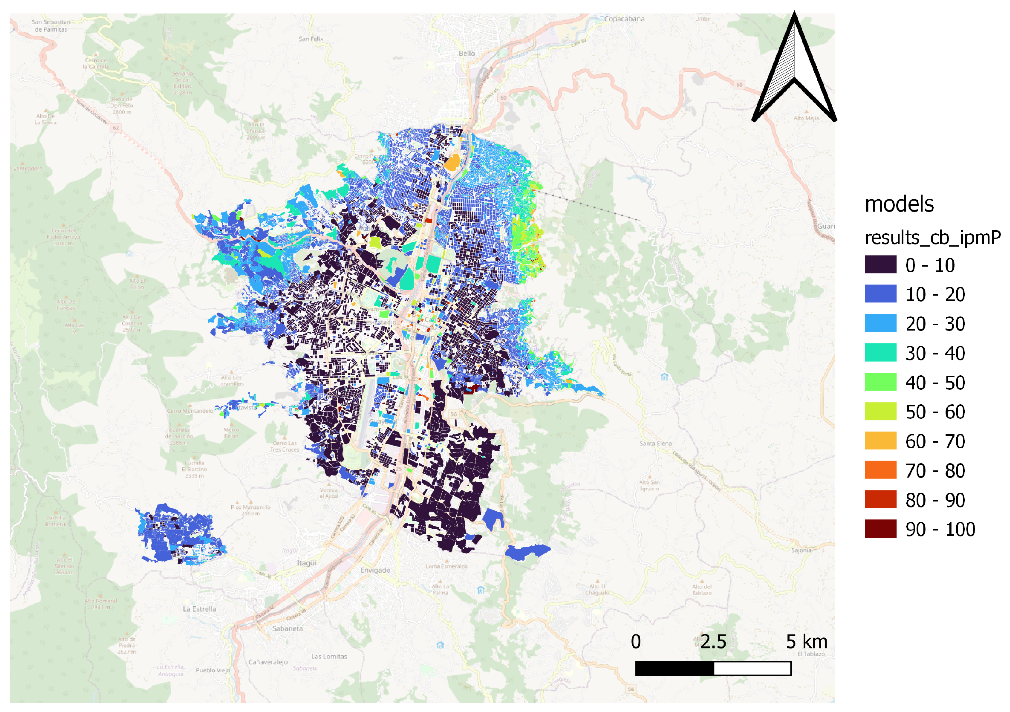
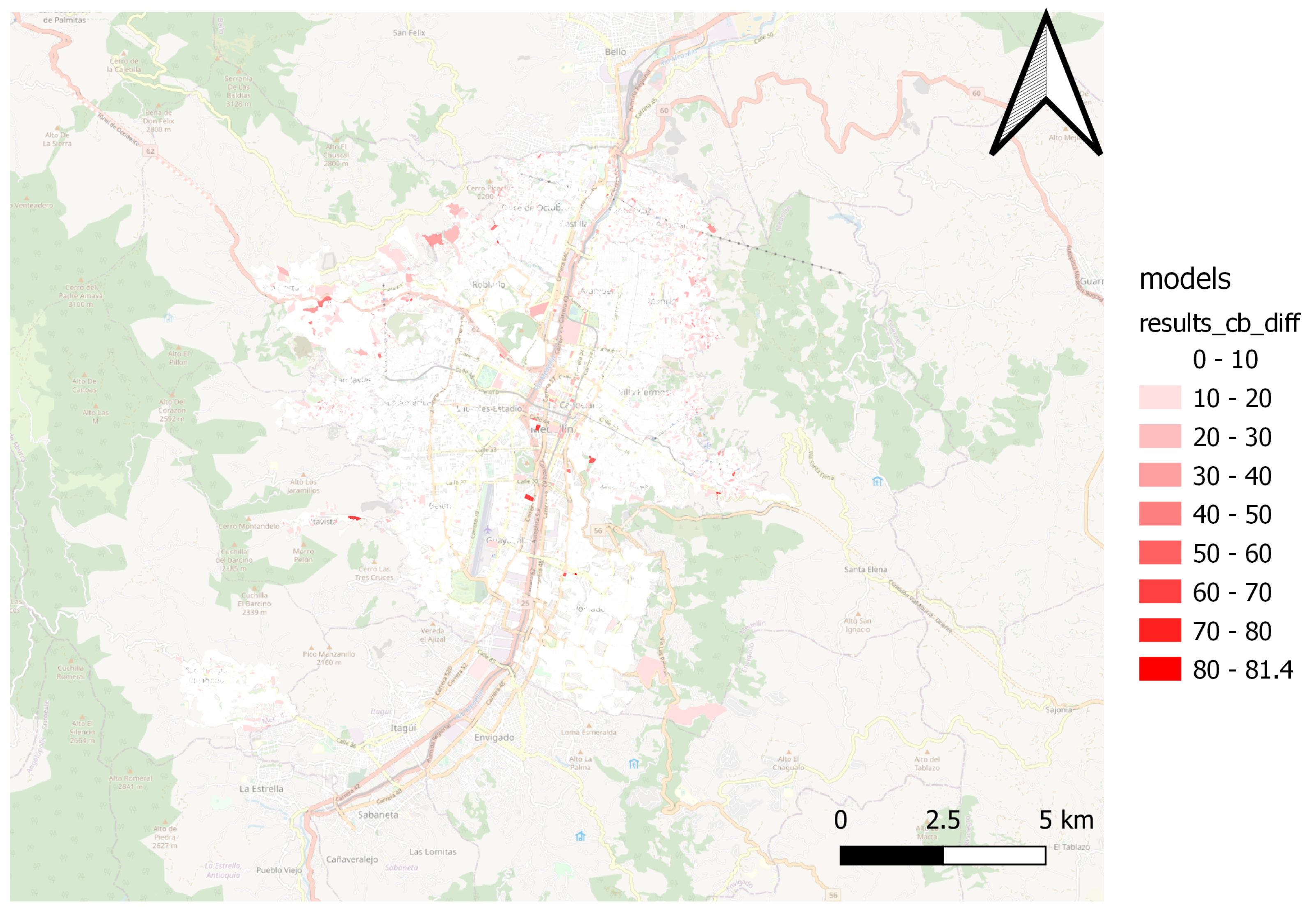
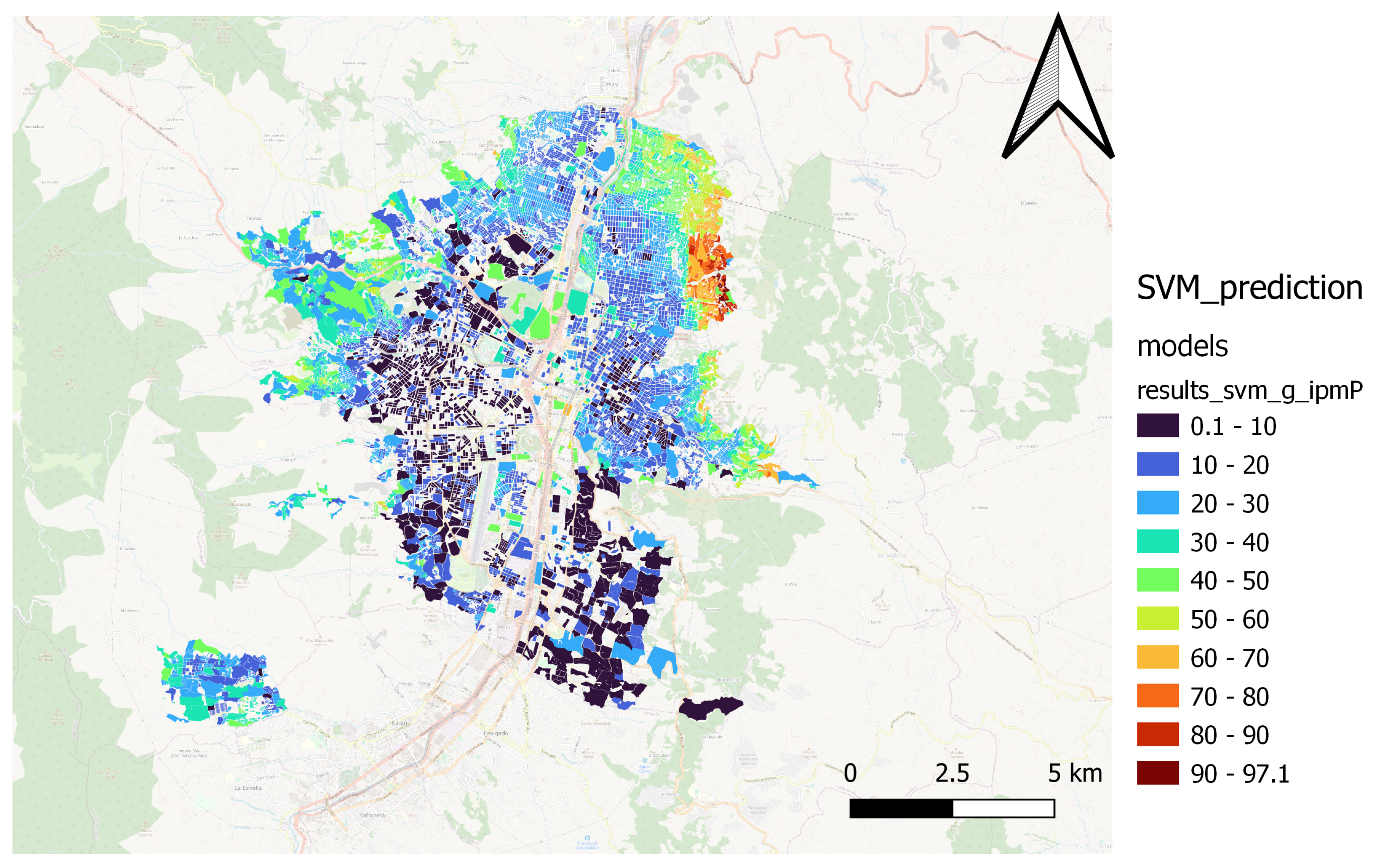
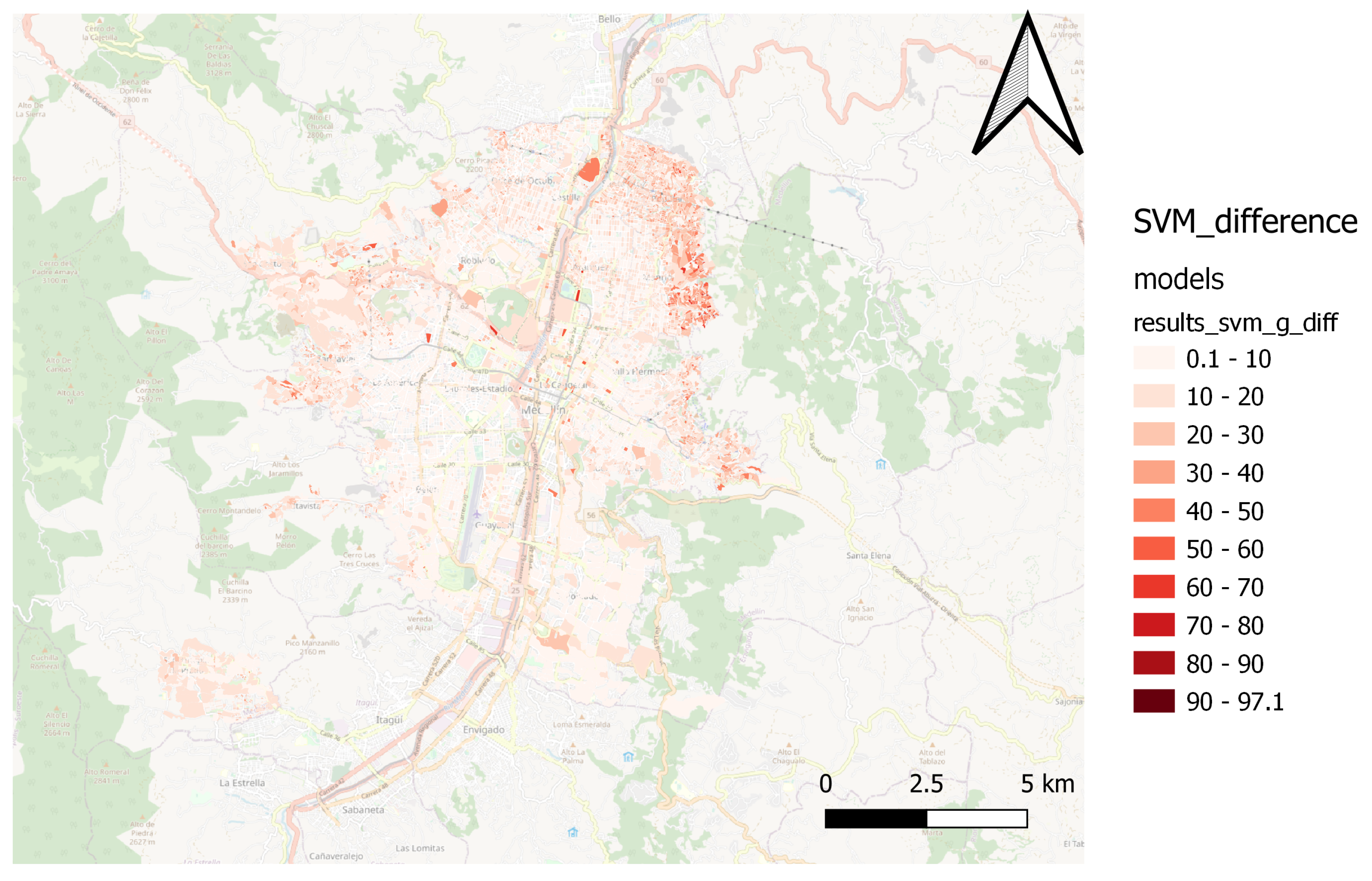
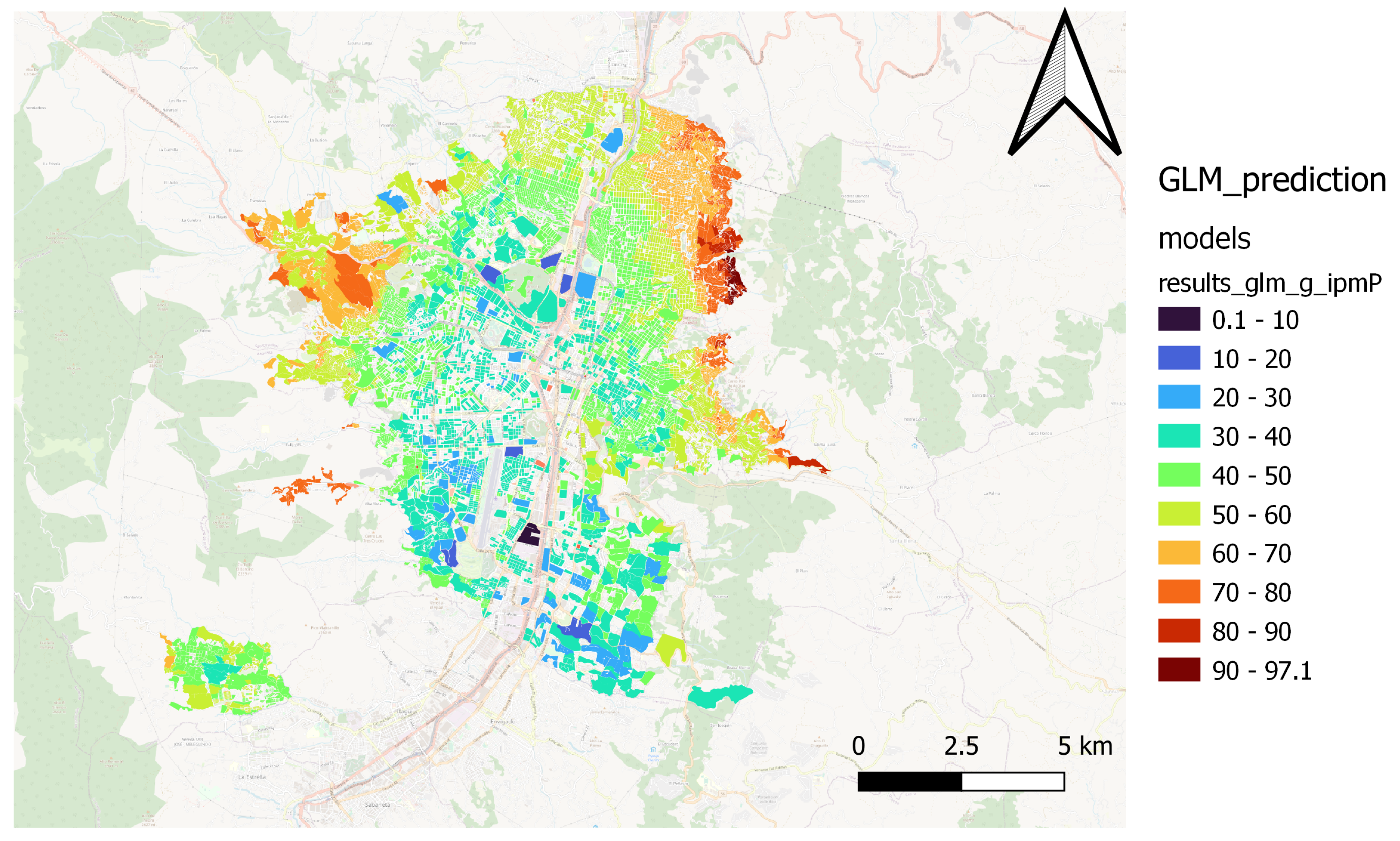
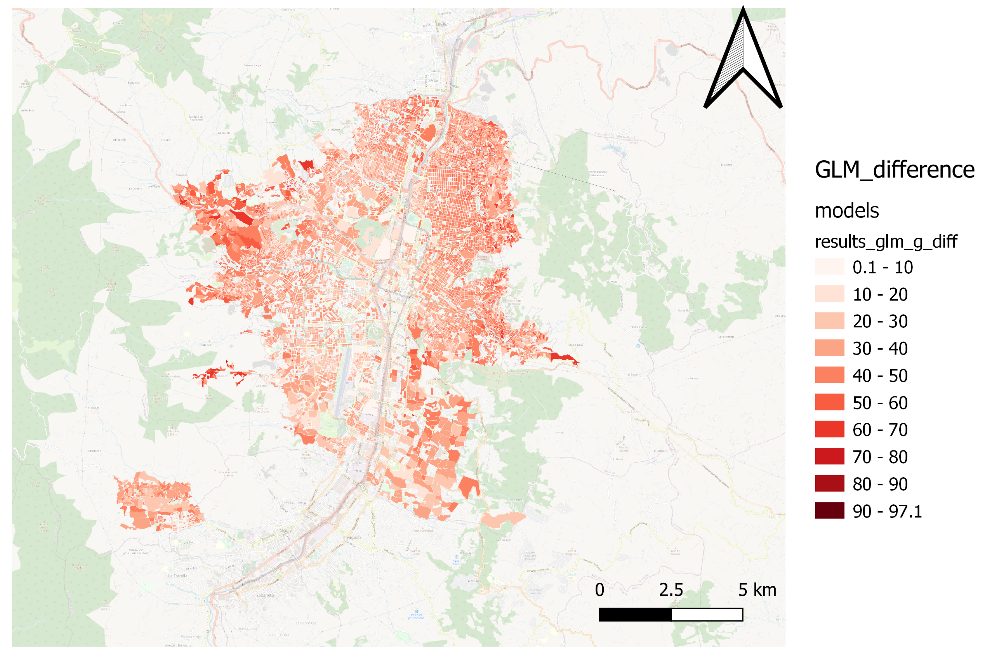
Through spatial comparison, it was possible to verify the capacity of various regression algorithms in estimating the MPI, as shown in Figure 4, Figure 5, Figure 6, Figure 7, Figure 8, Figure 9, Figure 10, Figure 11, Figure 12, Figure 13, Figure 14 and Figure 15 Specifically, Figure 4 and Figure 5 display the spatial distribution estimate of the MPI performed by the Random Forest and the difference between the ground truth MPI value and the estimated value. Figure 6 and Figure 7 illustrate the same conditions for the XGBoost model, Figure 8 and Figure 9 do so for the lightGBM model, and Figure 10 and Figure 11 show the performance of the Catboost model. The SVM model’s performance is shown in Figure 12 and Figure 13, while Figure 14 and Figure 15 show the GLM model’s performance.

The Catboost and Random Forest(1) models present a better fit for the spatial patterns of the MPI. Those models can estimate the result of the territories located in northern, northwestern, and northeastern peripheral areas, where most people in multidimensional poverty are concentrated. Furthermore, the models capture the spatial pattern in the city’s center and south.

With the Random Forest model 1, the most important variables are shown. The primary variable was population density, followed by block location; another important variable was the one created to separate hillside areas from middle and downtown areas. Two other variables that stand out in importance, although to a lesser extent than those mentioned, were land use, specifically the built-up and tree cover area. After those land use variables, variables such as the proximity to 5 km of transport and the police station, as well as 500 m from a church, are the variables that follow in order of importance. Variables that have less of an impact on the model estimation are those that are associated with a distance of 100 m from the center of the cell.

5. Discussion

Several studies predict poverty using spatial data, and many of them have already been presented in the related works section. This paper focuses on predicting poverty at a granular level using various spatial data sources that are freely available and easy to obtain. Additionally, six machine learning methods are compared for this purpose. The paper predicts the MPI using spatial data, which differ from the commonly used poverty indicator in the spatial poverty prediction literature, namely income, consumption, or the international wealth index (IWI) from Demographic and Health Surveys (DHS) Ayush et al. (2020); Blumenstock et al. (2015); Engstrom et al. (2017); Jean et al. (2016); Ledesma et al. (2020); Lee and Braithwaite (2020); Li et al. (2022); Sheehan et al. (2019); Steele et al. (2017); Watmough et al. (2019). The granular scale analysis implemented in this study allows multidimensional poverty to be estimated better at a level close to the citizen’s household.

The results show that the random forest algorithm yields the highest predictive power; this is a result that is in alignment with other poverty studies Browne et al. (2021); Hu et al. (2022); Liu et al. (2021); Puttanapong et al. (2022) and also with the review conducting by the World Bank, where it was suggested that the Random Forest algorithm could contribute to better poverty predictions Sohnesen and Stender (2017).

In previous exercises to predict the MPI for the whole country, Colombia’s national statistics department used satellite night-light images as predictors. The best accuracy measured by RMSE was equal to 0.7818. The approach utilized in this study focused on a single municipality. However, the result showed improved precision indicators’ performance, indicating this approach’s potential effectiveness in similar contexts (the minimum RMSE was 0.1094). In contrast to DANE predictions, the approach used in this study does not involve using neural networks. Instead, a simple model with fewer variables was preferred over a complex and black box predictor involving all of them. The results show that better performance can be achieved by using a few variables extracted from Open Street Maps and ESA’s land cover. Models were used to improve the metrics while maintaining interpretability.

The results show that combining different spatial data sources for predicting multidimensional poverty allows us to understand multidimensional poverty patterns at street block spatial-level detail. This is a necessary methodology to estimate poverty without relying on surveys commonly used for estimation. In the particular case of Medellín city, there is one primary data source to estimate the multidimensional poverty at the commune level (16 urban and five rural administrative areas). The data source is the city’s annual quality of life survey, which has a representative sampling at the commune level. Its annual cost is roughly $700,000 dollars at current 2022 Colombian prices. The quality of life survey conducted in 2021, and also the estimate of multidimensional poverty, was published in October 2022. In this regard, the block spatial level is more detailed than the commune and even neighborhood level frequently used in studies with social indicators in Medellín city. Chica-Olmo et al. (2020); Duque et al. (2015); Moya-Gómez et al. (2021). This intention of improving the spatial granularity is being carried out with promising results for poverty identification Hu et al. (2022) not to leave poverty data behind.

The results introduced show the capacity to broaden the perspective of identifying the population living in multidimensional poverty. Concerning the studies carried out in the city of Medellín, based on the use of satellite images for the identification of slum neighborhoods Duque et al. (2015), socio-spatial segregation with mobile phone data Moya-Gómez et al. (2021), and spatial analysis of quality of life Sepúlveda Murillo et al. (2019), this study complements the previous options, showing promising results to understand spatial inequities in the territories.

The findings of this study can be generalized to other territories with similar characteristics in terms of data availability. The methodology employed can also be used as a low-cost tool for policymakers to make informed decisions on poverty social intervention at the granular spatial level. However, it is crucial to note that further studies are necessary to improve the estimation of the MPI by extracting features from different sources and using more complex models to understand social–spatial patterns in the territory.

It is worth noting that the estimation can be updated automatically, thus eliminating the need to wait for a new survey. This process enables the estimation to be continually revised promptly and efficiently. However, it is essential to account for the inherent limitations of the proposed poverty estimation methodology in detecting circumstantial changes in poverty estimates.

The methodology proposed is limited to identifying multidimensional poverty arising from circumstantial changes in the economic and social system. For instance, the methodology introduced in this manuscript may not detect changes in poverty resulting from inflation, or the discontinuation of social assistance programs. As such, it is essential to recognize the current methodology’s contextual constraints and scope while interpreting the results.

6. Conclusions

This study implemented a method to predict the multidimensional poverty index in Medellín, Colombia, at the street block level. We obtained different spatial features freely available from Open Street Maps and ESA land use cover. The Random Forest, XGBoost, LightGBM, CatBoost, SVM, and GLM models were used to understand multidimensional poverty. The Random Forest algorithm achieved the highest performance, with an MAE of 0.07504. The spatial distribution of the multidimensional poverty estimate is highly correlated with the true values of the distribution. The first three variables of importance for the estimation of the random tree model were population density, block location, and an indicator variable that was created to separate hillside areas from middle and downtown areas.

This work is a promising result to extend the work to the whole country, given that the performance achieved is better than that reported by the national statistics department for estimating the MPI in Colombia. This research is in line with the efforts of the Colombian National Statistics Department to estimate multidimensional poverty in Colombia using spatial data. This is an opportunity for public policy to reduce the cost of collecting surveys and predicting zones where human access is difficult due to political and social restrictions. The methodology becomes a support tool to guide public policy decisions to achieve the Sustainable Development Goal of ending poverty in all its forms everywhere.

For future studies to improve the estimation of the MPI, it is possible to extract features from different sources and, through more complex models, join them together for the objective of prediction, for example, by using aerial or satellite images or even text and audio as multimodalities to understand social–spatial patterns in the territory. To improve the overall classification, future studies could focus on implementing algorithms such as convolutional neural networks that minimize the ambiguity between exposed soil and building structures such as rooftops, thereby enhancing the accuracy of the classification results. Or overlay the information between OSM’s polygons with spatial images in order to contrast if the land use definition is right.