Establishing Grounds for Building Orientation Mapping and Validation of Noise Level Correlation Modeling on Aircraft Take-off and Landing

Abstract

This research highlights correlation modeling between residential buildings orientation toward the runway as noise source and noise level. Many studies used noise mapping to identify noise performance in cities, but none of them discussed building orientation as an effort to reduce noise. This research aims to resolve the noise exceeding threshold of 55 dB for landed residential area. The method used was empirical experiments based on ISO 1996-1 using a 1:1-scaled building block model that was rotatable on its axis on various orientation angles. To examine the difference in sound reduction patterns, measurements were carried out during aircraft take-off and landing in three measurement conditions: outside the building model (OS), inside the model with both closed (CW) and open window (OW). The relative values of sound reduction in every angle were mapped and a Correlation Modeling was then empirically developed and theoretically validated by origin-8 software. As a result, the empirical validation formula deviation averaged only 1.20% and 1.13% during take-off and landing respectively from the actual noise and the theoretical validation. Furthermore, the new modeling was verified as a derivation from the grand theory of inverse square law and could be applied for master plan design.

1. Introduction

Aircraft noise is a serious problem for the quality of life of building inhabitants surrounding the noisy airport for many decades [1,2,3]. Building orientation without considering environmental acoustics causes a high level of sound received and it could disturb human life [4]. Occupants would be annoyed by the aircraft noise because, based on the regulation and findings of research, the quality standard of noise level on dwelling is 55 dB(A) [4,5,6], 30 dB(A) inside a dwelling at night [7], 50 dB(A) and 40 dB(A) in open window dwelling during daytime and night, respectively [7]. This study focused not only on how the building should be placed on term of orientation toward the runway, but also to what extent the validation of correlation modeling between the orientation angles and noise level received by occupants could be established. The first research by Erni and Anggana (2013) only examined the construction of building materials that can reduce noise [8], while Erni in 2013 conducted modeling research based on airport housing case studies, but it did not have any detailed discussion about sound level patterns and sound reduction values when aircraft take-off and landing as well as the empirical modeling validation [9]. A study by Erni and Trilistyo (2015) revealed the aspect of climate in noise reduction patterns occurred in the housing near the airport [2]. None of these studies discussed the noise change, relative value and correlation modeling validation based on the aircraft take-off and landing. This research highlights the building orientation mapping toward the runway as noise source in airport and the correlation modeling as well as validation of correlation modeling in both theoretical and empirical ways that have not been previously published elsewhere. The correlation modeling and validation have been conducted to ensure that this new theory could be applied and generalized in the building’s layout. With this new theory, architects and urban designers could design building layout that has the capability of reducing noise from the aircraft while take-off and landing.

1.1. Aircraft Noise Impacts to the Environment and Buildings

As the aircraft noise is a particular nuisance on take-off and landing, it has become a curious topic of research in the recent decades. Many studies have observed the aircraft noise on their own ways [6,10,11,12,13,14,15]. A research discussing the aircraft noise exposure to population near the airport has been observed by Gani et al. [6]. This research developed mathematical modeling and algorithm assigning aircraft operational procedure in Belgrade Airport that could reduce number of noise exposed population. The study used numerical air traffic assignment model to predict the noise exposed population reduction. As a result, in the proposed model, the numerical modeling on the aircraft assignment could significantly reduce the noise exposed population, but it had consequences especially on increment of fuel usage [6]. Similar to Ganis’ study, research conducted by Ozkurt et al. [10] discussed the impact of aircraft noise to human health. In the study, they proved that the noise caused serious illness such as hypertension and sleeping annoyances on the occupants especially in the north side of the Izmir Adnan Menderes Airport where the city center is located. Using the Sound-Plan 7.2 software and ECAC Doc-Interim methods, the study predicted aircraft noise. Ultimately, the results recommended the airport authority to control the airport capacity with better flight schedule system [10]. On the other hand, other research conducted by Licitra et al. used the Integrated Noise Model (INM) to predict the noise impact to the affected population in the vicinity of the Galileo Galilei Airport. Besides the INM, this study also used Automatic Identification System (AIS) signals to duplicate the aircraft noise on both take-off and landing [11]. This research not only explored the noise annoyance caused by the aircraft as similar to other studies [10,13,15], but also suggested the noise abatement procedures to the airport operator in case of the future development of the airport. In addition, none of the studies listed observed the impact of aircraft noise on buildings, and landed buildings layout suggestions correlated the noise anticipation and solutions.

As far as aircraft noise, research conducted by Camara et al. studied acoustical risks management to evaluate the noise impact on buildings close to the airport [16]. On their study, Camara et al. revealed that the closeness of housing to the Bamako airport in Mali and the exceptional aircraft noise during take-off and landing required assessment on the aircraft noise level, noise level exposure of occupants, and building components rapprochement to reduce the noise [16]. Although the research offered some solutions for buildings to control the aircraft noise, they did not reveal the buildings in the context of master plan design. In fact, the study hardly conducted the observation on the building layout as noise control strategy to solve the aircraft noise. The further question is to what extent the buildings near the noisy airport should be oriented so they will be safe and comfortable in terms of noise disturbances.

1.2. Procedures on Predicting the Aircraft Noise

The phenomenon of the aircraft noise is that low frequencies occur shortly after a plane take-off [17] and high frequency occurs when an aircraft is landing [18]. According to Harris and Piersol, airplanes emit noise exceeding the maximum threshold when above the head, then the noise level gradually decreases. Noise is dominated by a high frequency at landing and low frequency shortly after take-off. Within 10 seconds after take-off, low frequencies are emitted by jet components and spread through the atmosphere [1]. Many studies observed the aircraft noise and its impact to the built environment and occupant near the airport [16,19,20]. Sahai et al. quantified to distinguish aircraft noise in general, beyond conventional metrics of A (dB) Sound Weight Level or Effective Noise Level (EPNL) commonly used to assess aircraft noise [19]. Like Sahai et al., study conducted by Lu [21] combined the practical and theoretical methods on the aircraft noise measurements [21]. Meanwhile, Camara et al. studied risk assessment of buildings near the Bamako airport in Mali. Using field observation and acoustical pattern measurement inside the buildings, they concluded that buildings on the airport zones in the future should consider protection against noise interference, atmospheric emissions from aircraft, and the use of appropriate materials [16]. Furthermore, studies on the aircraft noise often relied on supporting data such as weather, height of aircraft, distance between sound source and buildings or occupants and noise mapping of airport areas [17]. Studies conducted by Harris and Piersol (2002), Ignaccolo (2000), Aparecida et al. (2014) used L A_eq methods for predicting the aircraft noise [1,18,22].

1.3. Noise Control on the Aircraft Noise

Several studies have highlighted the ways to anticipate the disturbing impact of the noise, offering solution for noise control to reduce the aircraft noise [10,11,13,14,15]. In such studies, the population near the airport is the most affected aspect that needs the noise reduction to improve their quality of life. Several diseases occurred by the aircraft noise such as hypertension, cardiovascular, and sleeping disturbance were most prevalent problems that needed to be both anticipated and decreased. In addition, studies conducted by several researchers have revealed active and passive noise control in buildings [23,24,25]. As the means of aviation capacity growths by 10% every year in China and at about 3% hearing loss exposure to aircraft noise, Xie et al. [23] observed the aircraft noise impact to the psychological system and cardiovascular in human. They revealed that the increment of flight capacity and airport expansion could cause the growth of areas and populations annoyed by the noise. In the results of the study, they suggested several active and passive noise control such as purchasing noise detection equipment, installing sound insulation in residential buildings surrounding the airport, directing the airport expansion far away from the local community, and improving preventive legislation in China on aircraft noise control [23]. The interesting study conducted by Pamies et al. [24] proposed an active noise control on aircraft with bottom hinge window openings that can reduce sound transmission by 3 dB(A). A window model was placed in the living façade closest to the airport, then active controls are configured to reflect the pressure emitted by the aircraft using a single-input feed forward adaptation system [24]. On reducing noise by window innovation, Park and Kim proposed the model of airtight window. As it is known that most windows in Korea has double frame and air gap, the window construction influences the thermal and acoustics performances. By the insulation model between the outer and inner frame, the noise could be reduced up to 10 dB, so the model could be applied for the apartment near the airport [25]. Furthermore, many studies were also observing the aircraft noise in terms of the urban solutions.

In addition, in terms of studies on noise control in urban areas, there were several studies performing noise control in urban [26,27,28,29,30,31,32]. Noise mapping has an important role to indicate noise exposure in the urban scape. A study of noise performance in Santiago city conducted by Suarez and Barros used software of CadnaA, Computer Aided Noise Abatement. The software contains important data of cartographic and traffic flow rates. Remarks revealed from the research was that there had not been identification on noise levels in various or specific parts of cities as well as any solutions to reduce the noise especially for functions such as residential areas, hospitals and schools. The noise mapping was also used in study performed by Cai et al. [27] and Tsai et al. [28]. The differences were on the methods and results. Cai et al. used Geographical Information System (GIS) and Global Positioning System (GPS) [27], while Tsai et al. not only used GIS, but also 345 stations monitoring noise level in Tainan, Taiwan. The results showed that, although the GIS procedure showed an accurate precision on the data, there was a gap of 2% between field measured and predicted data [27]. Meanwhile, the study identified about 90% of inhabitants in Tainan city suffered from noise, in such a way that the Taiwanese government sought solution to reduce the noise in the city [28]. Similar studies used noise mapping and GIS to describe and identify the noise in cities [28,29,30]. The studies discussed used noise mapping in cities that is very important to identify noise emitted by road traffic and might be good solutions to arrange spatial planning related to design block of building in many parts, but none of the studies discussed correlation modeling based on the noise mapping in cities. The recent study not only used noise mapping on the region near the airport, but also established a theoretical correlation model between noise and building orientation especially in the buildings surrounding the noisy airport.

2. Materials and Methods

This research investigated a housing estate near Achmad Yani International Airport, Semarang, Central Java, Indonesia. One of the housing clusters in the estate was very close to the airport runway. The noise from the airport annoyed the occupants of the residential buildings all day long. The following image indicates the noise mapping of the airport (Figure 1) and close proximity of the housing cluster to the runway (Figure 2).

The Figure 1 not only shows the noise mapping of the International airport in Semarang, but it also describes how the dwelling houses surrounding the airport must receive remarkable aircraft noise all day long, especially during the aircraft take-off and landing. The proximity of dwelling to the runway as noise sources have to be assessed due to the occupants’ noise exposure. On the image, the landed residential buildings on the north, south and west parts of the airport zone have received the highest noise level of approximately 90–100 dB(A). To solve the problem of the aircraft noise and to consider the research background, this current study focused on how the buildings should be oriented toward the noise source and what modeling could be used to place the building on-site appropriately.

The Figure 2 illustrates the dwelling cluster near the airport runway as a critical point during the aircraft take-off and landing. Because the sound sources were identified from flight schedule in the airport, a measurement with a rotatable building model located in the distance of 340.2 meters from the runway was used to map the relative value of sound reduction in every 30° and 45° orientation angle. The building model was also built in mass configuration represented the real building block in the field. Due to the high and low frequencies on the aircraft flight during take-off and landing, the building mass configuration aimed to observe the noise wave symptoms.

Represented as orientation facing to the runway, the building model was used to control the effectiveness of α rotated orientation on reducing noise by comparing noise level of building with rotated α and building with 0° orientation (see Figure 3a). The ratio value between them was defined as Relative value (R_V). Figure 3b shows the measurement procedure with the null α oriented building as control model and building block model which was rotatable on its axis to observe the noise level decrease pattern in every 30° and 45° orientation angle (see Figure 3b). The wall in front of the rotatable building model represented the building block in real condition.

Such a measurement could be rotated on its axis with 16 various angles ranging from 0°, 30°, 45°, 60°, 90°, 120°, 135°, 150°, 180°, 210°, 225°, 240°, 270°, 300°, 315° and 330° (see Figure 3b). Meanwhile, other measurements were carried out in three conditions covering outside the building and inside the building either in open or closed window condition during aircraft take-off and landing in order to examine the difference sound level patterns and the effectiveness of rotation occurring in the building model (see Figure 3a,b).

To make the model has Sound Transmission Loss to an existing building, the model was layered by styrofoam sheet, carpet, and coir composite, creating an acoustical capability of the model to represent the building in real conditions (Figure 4), in that the building model was fitted in the location with a distance to runway for only 340.20 meters.

Furthermore, to observe the noise pressure level and climate data, this study used several measuring instruments, as listed in

Table 1. Measuring instruments used in the current research.

Instruments	Unit of Tools	Branded
Sound Level Meter	2	Luthron SL-4001 Calibrated number F80550 & G18304
Dry-wet thermo-hygrometer	1	Krisbow KW06-561
Thermo-Anemometer	1	Extech AN-100
Stopwatch	2	Pursun PS-08
Camera Digital	1	Canon EOS M-100
Laptop	1	ASUS W 5FM, CPU Duo T5500 Memory 512 MB

.

The aircraft noise is a comprehensive transportation noise covering wide broadband frequencies [19]. Moreover the noise has fluctuative amplitude which causes it to be more complex [19]. Although it has complexity, this study focus on the human exposure especially on its impact to orientation in buildings surrounding the airport. For this aim, this present study did not used frequency analyzer [22], and instead of this, the validations were used to verify the theoritical correlation model. The measurement with a time span of 2 minutes per 3 seconds had been used due to its tightly hyperbolic curve graph. As used in a number of studies, the equivalent sound pressure level obtained in the range of 2 minutes per 3 seconds was calculated based on ISO 1996-1 by the following equation (see Equations (1) and (2)) [1,22,34]. This traditional procedure of Equivalent A Weighted Noise Pressure Level was also used in the study conducted by Filippone [35]. This procedure did not use frequency analyzer, due to the aim for obtaining the noise exposure on human impairement. Although this method is still polemic in several studies [7,36,37], the rest of the studies have shown that this method is a simple way for observing the outdoor noise:

$$L_{eq}=10lo{g}_{10}\frac{1}{N}{\displaystyle \sum }{n}_1{10}^{0.1L_i}$$

(1)

$$L_{eq}=10lo{g}_{10}\frac{1}{T}{\displaystyle \sum }{t}_1{10}^{0.1L_i}$$

(2)

with n being the number of events with the level of L_i, N is the total number of events and T_i is the duration of time at the level of the sound L_i, while T is the total time span. The goal of this formula was to obtain the average sound level value within a certain measurement period. Because the sound source of the research was the sound of aircraft moving linearly on the runway up to a certain height, the sound level measurement used the L_eq method as described by such formula. To calculate sound reduction due to the distance factor in an open space, decibel units or Watt/m² units were used as shown in Formulas (3)–(5). When using a formula with Watt/m² units, the results must be converted to decibel units, using the Formula (4). The formula has also been used by a number of researchers in previous studies [1,18,22]:

$$\frac{I_1}{I_2}={\left(\frac{r_2}{r_1}\right)}^2$$

(3)

$$L=10\log \left(\frac{I}{I_0}\right)$$

(4)

$$L_2=L_1-10\log \left(\frac{r_2}{r_1}\right)$$

(5)

where L₁ and L₂ are the noise levels in the distance r₁ and r₂ respectively to the source of the decibel sound, and I₁ and I₂ are noise intensities at distances r₁ and r₂ respectively in Watt/m². r₁ and r₂ are the distance from the L₁ and L₂ sound sources respectively to the receiver (m). To determine and map the level of noise reduction between the control model (0°) and the observed model (α) on the noise level, the following Relative Value formula is used:

$$R_V=\frac{L_{\alpha }}{L_0}$$

(6)

where R_V is the relative value of noise level reduction (see Equation (6), L₀ and L_α are sound levels received in the model with orientation angle 0° and α° respectively (decibel)). By getting the relative value of the sound level change, the orientation angle rating was determined, starting from the angle that most effectively reduced the sound level to the angle that increased the sound level. Sound level change rating was obtained by using the Comparative Test of Average Difference (Compare Means). The following method was applied both during aircraft take-off and landing:

$$\overline{R_V}=\frac{{\displaystyle \sum }{R}_V}{{\displaystyle \sum }x}$$

(7)

where $\overline{R_V}$ is the average of relative value, ${\displaystyle \sum }R$ is total Relative value per building orientation angle, and ${\displaystyle \sum }x$ is total measurements per building orientation angle. To simplify the understanding of how the Relative Value Rank could be found from the total measurements,

Table 2. The Relative Value Mapping and Rating Procedure.

Aircraft Condition	Measurement Condition in Building	Code	Number of Angles × Data	Equation Used	Results
Take-off	Outside	OS-T	16 × 40 = 640 data	$\sum R/\sum x$	Mapping and Ranks
	Inside-closed window	CW-T	16 × 40 = 640 data
	Inside-opened window	OW-T	16 × 40 = 640 data
Landing	Outside	OS-L	16 × 40 = 640 data	$\sum R/\sum x$	Mapping and Ranks
	Inside-closed window	CW-L	16 × 40 = 640 data
	Inside-opened window	OW-L	16 × 40 = 640 data

describes the calculation procedure to determine the Relative Value (R_V) from the building orientation mapping and rank for three conditions: outside, inside closed window, and inside open window during both aircraft take-off and landing.

The measurements were taken within 4 weeks. There were various types of aircrafts, but the calculation of Relative Value (R_V) is a comparison between noise level of rotated model and that of control model. Although the aircraft types were vary, the value of R_V was a relative value rather than an absolute value. The development of the correlation mathematical modeling either between sound levels and orientation angle or climate and noise level were analyzed by polynomial goniometric regression curve with the help of Origin-8 software.

The construction of the correlationship model was created using the fitting model method. The fitting model is a stage of calculating the estimated parameters or regression coefficients based on the chosen and method. The coefficients were then tested to see whether or not they were significant as model parameters. The coefficient is significant if at a certain level of confidence, and the value is considered not equal to zero. At the final stage of the study, a model of the empirical relationship between the noise level and the orientation angle obtained was validated, both theoretically and empirically.

3. Results

Since air traffic activities has become a tremendous noise in cities, several studies focused on impacts of airport noise and description on how to reduce the noise exposure in populations around the airport [5,6,10,11,12,14,15,18]. To explore any solutions on the noise abatement procedures around the airport, the scientists used noise mapping with various methods. Sometimes they used several softwares to make the noise mapping in cities such as Cadna-A, Sound-Plan, GIS and GPS, once the map had been available as parts of building and environment spatial planning documents in local government, for example, see Figure 1 in previous subheading.

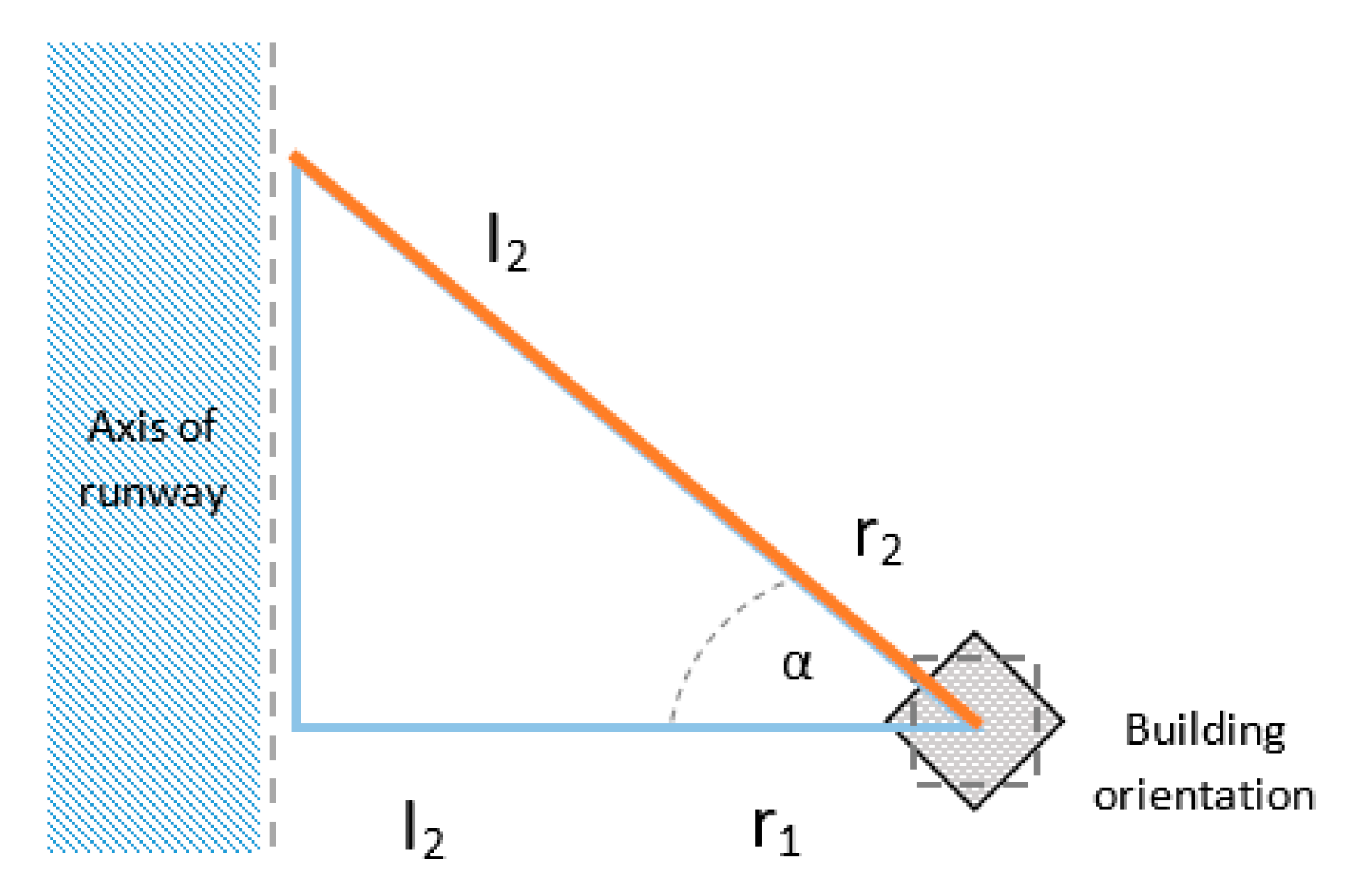
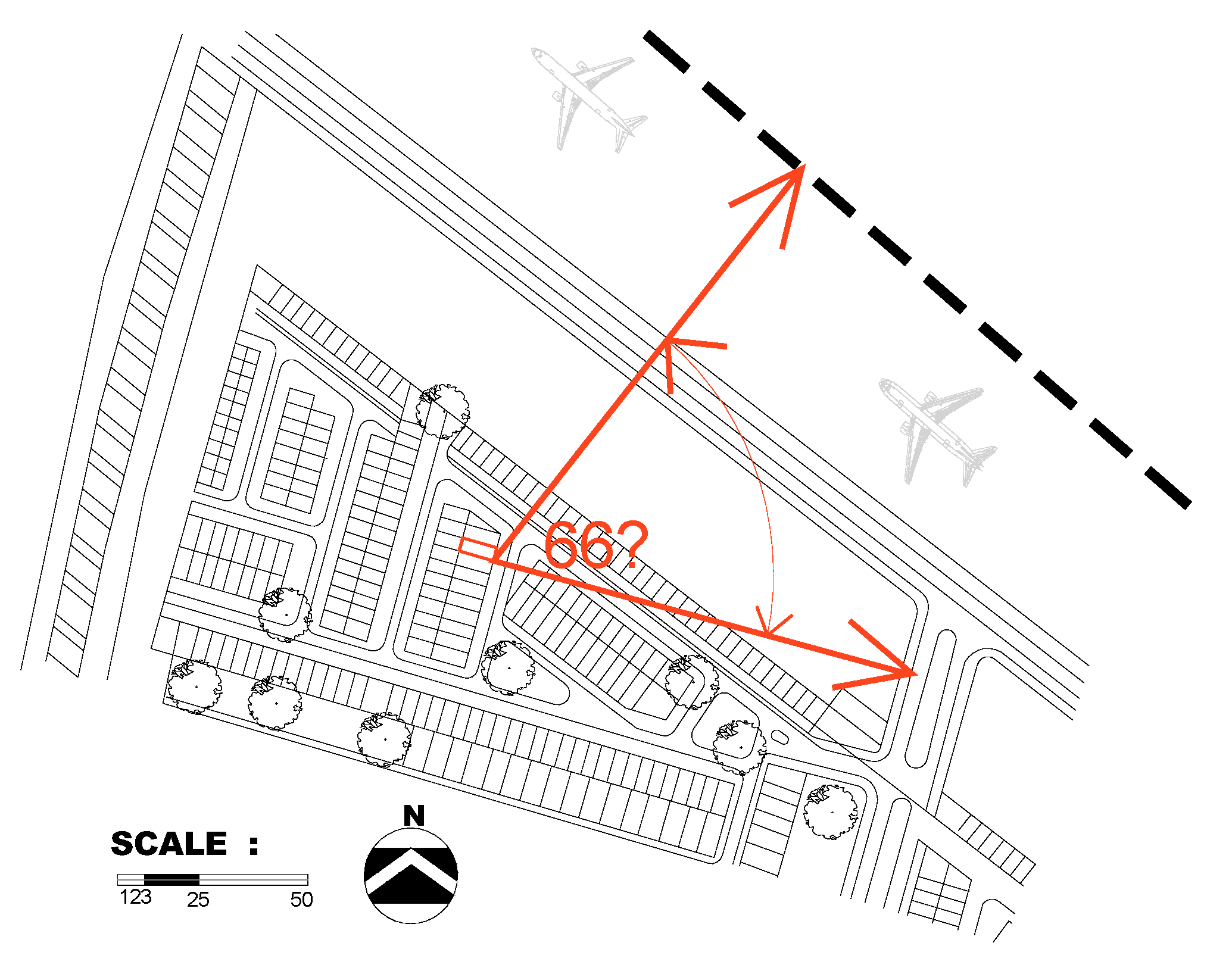
3.1. Relative Value (R_V) for Establishing Building Orientation toward Runway

The main purpose of this research is to develop Relative Value (RV) using various orientation angles and establishing curve estimate fitting based on empirical noise measurement. First of all, a 1:1 scaled rotatable building block model was created to observe the noise level pattern on buildings created by the aircraft noise. The building block model was then located in the closest residential area of only 340.2 meters from the airport runway. Comparing the noise level received by the un-rotated control model and those received by the rotatable building block model generated the relative value data. To observe the noise level pattern comprehensively, the field measurement was conducted during aircraft take-off (T) and landing (L). Moreover, to observe the noise pattern in buildings, the aircraft noise level in building block model was measured on three conditions covering outside the model (OS), inside the building model, for both closed window (CW) and opened window (OW). As a result, the relative values are described in

Table 3. The Average Relative value (R_V).

Building Orientation towards Runway	Number of Measurements	Take-off			Landing
		Outside (OS-T)	Closed Window (CW-T)	Open Window (OW-T)	Outside (OS-L)	Closed Window (CW-L)	Open Window (OW-L)
0°	40	0.922	0.861	0.954	0.919	0.856	0.961
30°	40	0.883	0.793	0.953	0.880	0.784	0.957
45°	40	0.861	0.751	0.967	0.870	0.770	0.941
60°	40	0.900	0.828	0.963	0.893	0.807	0.968
90°	40	0.855	0.740	0.956	0.829	0.697	0.969
120°	40	0.841	0.877	0.936	0.821	0.685	0.952
135°	40	0.834	0.703	0.940	0.802	0.655	0.951
150°	40	0.854	0.746	0.935	0.828	0.689	0.949
180°	40	0.950	0.916	0.918	0.827	0.692	0.903
210°	40	0.861	0.750	0.962	0.857	0.742	0.960
225°	40	0.928	0.878	0.939	0.849	0.730	0.941
240°	40	0.862	0.751	0.952	0.873	0.771	0.955
270°	40	1.041	1.076	0.967	0.976	0.965	0.962
300°	40	0.898	0.827	0.967	0.828	0.715	0.963
315°	40	0.954	0.922	0.967	0.955	0.920	0.963
330°	40	0.961	0.930	0.972	0.957	0.957	0.956
Average of RV		0.900	0.834	0.953	0.873	0.777	0.953

.

Both at the time of the measurement position outside and inside the building (take-off and landing), the lowest Relative Value (R_V) is in the orientation 135° toward the runway. At opened window measurement, the lowest Relative Value (R_V) is in the orientation 180°. These symptoms are the results of sound radiation reflection and absorption in the building mass configuration. Changes in sound behavior are caused by reflection, diffraction and absorption of sound wave at both high and low frequency when the aircraft is in take-off and in landing, as well as building mass configuration (see Figure 5). On the measurement inside the building model, the noise level received is not only influenced by the environment, but also affected by repetitive reflections and absorption of the enclosure elements covering, wall, ceiling and floor (see Figure 5 on the orientation 180°). On the contrary, during measurement outside the building, the noise is only influenced by the environment and another building block configuration. For further detail, see Figure 5 below.

Based on the empirical data in Table 3 and Figure 5, the building orientation mapping could be depicted to generalize the noise level phenomenon on the building surrounding the airport. Figure 6 illustrates the building orientation mapping generalization related to the Relative value (R_V).

Building orientation mapping is identically presented as a noise-mapping zone, as shown in Figure 6. The noise mapping is categorized into two zones: (1) the effective zone is the zone which has Relative value between 0.529 to 0.945, where the noise level emitted from the aircraft could be reduced as much as 5% to 47% or 2–20.9 dB(A), and (2) the ineffective zone has Relative value at about 1.011 to 1.593. The relative value in this zone means the orientations in red zone (see Figure 6) tend to enhance the noise level as much as 1–59% or at about 3.1–17.7 dB(A).

3.2. Correlation Modeling between Orientation Angle (α) and Noise Level

This research aimed to formulate the correlation modeling between the orientation angles of building and the noise level received in building in three condition covering outside the building (OS), inside the building with closed window (CW) and inside the building with opened window (OW). In addition, the data were obtained during aircraft take-off and landing in average and maximum value model. The following discussion reveals a summary of noise pressure level received and modeling curve estimate as correlation modeling based on the field measurements.

3.2.1. Aircraft take-off

The data in the field measurement is summarized in Table 2 including three conditions during aircraft take-off and landing. The aircraft noise was also influenced by the climate data covering temperature (°C), humidity (%) and wind velocity (m/sec). The development of the correlation modeling L = f(α) with the Goniometric Curve Estimate Regression analysis method for the condition at take-off coverings conditions of outside the building (OS-T), inside the building-closed window (CW-T) and inside the building at open window (OW-T). The summary of the noise level at take-off on the three conditions is provided in

Table 4. Summary of average sound pressure level during aircraft take-off.

α	OS (Outside the Building)				CW (Closed Window)				OW (Open Window)
	Leq (dB)	T (°C)	RH %	V m/sec	Leq (dB)	T (°C)	RH %	V m/sec	Leq (dB)	T (°C)	RH %	V m/sec
0°	79.00	28–32	70	5.0	50.05	28–32	70	5.0	63.85	27–30	72	5.0
30°	66.38	27–33	60	4.8	37.43	27–33	60	4.8	63.70	27–30	79	5.0
45°	61.15	27–33	60	4.0	32.20	27–33	60	4.0	63.80	29–33	92	6.0
60°	69.65	27–33	60	4.0	40.70	27–33	60	4.0	62.29	25–27	80	7.0
90°	67.51	31–36	60	5.0	38.56	31–36	60	5.0	64.48	28–31	80	1.5
120°	62.03	28–32	72	5.1	33.08	28–32	72	5.1	63.54	30–35	65	1.7
135°	60.24	27–30	75	4.6	31.29	27–30	75	4.6	62.34	30–35	65	5.0
150°	61.69	26–27	90	3.6	32.74	26–27	90	3.6	62.96	30–35	70	1.8
180°	66.85	29–34	70	5.0	45.45	29–34	70	5.0	65.75	28–31	72	4.5
210°	63.83	30–37	55	4.5	34.88	30–37	55	4.5	61.68	31–37	70	12.0
225°	70.67	29–35	55	8.7	41.72	29–35	55	8.7	66.36	28–32	65	8.0
240°	60.74	29–35	55	4.0	31.79	29–35	55	4.0	70.34	28–32	65	8.0
270°	81.44	28–31	80	11.0	52.49	28–31	80	11.0	62.29	29–31	70	2.0
300°	70.79	27–30	80	7.4	41.84	27–30	80	7.4	62.96	27–29	90	1.5
315°	72.66	25–26	92	0.3	43.71	25–26	92	0.3	64.76	30–36	75	4.0
330°	63.89	27–30	82	4.0	34.94	27–30	82	4.0	62.86	30–36	75	3.0

.

The next step after capturing the noise level data at take-off on the three conditions was developing the correlation modeling between orientation angles and noise level received at building block model. The correlation modeling was carried out during take-off and landing by selecting the type of aircraft to Boeing 737-200 as either the highest noise level of others or the most frequent flyer on flight schedule. Consequently, it was found that the selected data were analyzed by curve estimate fitting method using Origin-8 software. The

Table 5. Maximum L_eq at OS-T [9].

α (°)	Leq (dB)
0	90.10
60	80.90
180	86.70
210	74.80
225	82.70
270	86.30
315	83.7

$L=L_0+A\ast \sin \left(\pi \ast \left(\alpha -{\alpha }_c\right)/\omega \right)$. $R^2=0.841$

and Figure 7 describes the modeling process in the Origin-8 graphs in which the L_eq data were selected from Boeing 737-200.

Figure 7 shows the example of sinusoidal curve presented the correlation modeling between the orientation angle and noise level received at the building block model, which was similarly applied for other conditions either at take-off or landing. By using the curve estimate fitting methods, the correlation modeling could be established as:

$$L=L_0+A\ast \sin \left(\mathsf{\pi }\ast \left(\alpha -{\alpha }_c\right)/\omega \right)$$

(8)

where A is amplitude, π/ω is constant, α is orientation angle in (°), and $\pi \ast \left(\alpha -{\alpha }_c\right)/\omega$ is a phase. To clarify the results of the development analysis of the orientation aspect model on the condition at take-off, it is necessary to present a summary table of the following relationship models (

Table 6. Summary of Correlation modeling during aircraft take-off.

Condition	Noise Level	R2	L=L0+A∗sin(π∗(α−αc)/ω)
			αc	w	A	L0
OS-T	Average	0.729	29.647	11.934	3.913	58.834
	Maximum	0.841	63.081	41.826	7.173	83.381
CW-T	Average	0.729	29.647	11.934	3.913	30.144
	Maximum	0.841	63.081	41.826	7.173	54.431
OW-T	Average	0.819	−92.854	149.866	1.010	63.037
	Maximum	0.929	166.021	132.151	3.045	73.150

):

Table 6 shows that each variable in the formula is explained by the notations α_c, ω, A, and L₀ in each condition, both in the conditions of OS-T, CW-T and OW-T. The greatest R² value at the aircraft take-off is the OW-T conditions with 0.819 and 0.929 in average and maximum respectively which means that the correlation of orientation angle and noise level in OW-T is the strongest than other conditions.

3.2.2. Aircraft landing

The explanation of the development of correlation modeling at the aircraft landing has a similar structure to the previous explanation for aircraft take-off. The modeling analysis consists of three conditions covering outside the building (OS-L), inside the building-closed window (CW-L) and inside the building-open window (OW-L).

Table 7. Summary of average sound pressure level at landing.

α	OS (Outside the Building)				CW (Closed Window)				OW (Open Window)
	Leq (dB)	T (°C)	RH (%)	V (m/sec)	Leq (dB)	T (°C)	RH (%)	V (m/sec)	Leq (dB)	T (°C)	RH (%)	V (m/sec)
0°	62.86	28–32	70	5.0	33.91	28–32	70	5.0	61.45	27–30	72	6.0
30°	60.11	28–33	60	3.0	31.16	28–33	60	3.0	61.70	28–30	83	6.0
45°	58.13	27–33	60	3.0	29.18	27–33	60	3.0	65.69	28–32	75	6.0
60°	60.43	27–33	60	4.0	31.48	27–33	60	4.0	61.56	28–29	80	0.2
90°	57.72	30–32	90	10.5	28.77	30–32	90	10.5	62.77	30–32	85	0.9
120°	54.97	28–35	70	4.5	26.02	28–35	70	4.5	60.92	28–33	65	0.5
135°	55.10	27–29	85	6.6	26.15	27–29	85	6.6	60.85	29–34	70	5.0
150°	65.19	26–27	90	3.6	36.24	26–27	90	3.6	60.77	28–33	70	3.0
180°	55.25	27–31	65	4.2	26.30	27–31	65	4.2	57.88	28–31	72	4.5
210°	56.63	28–34	70	5.0	27.68	28–34	70	5.0	61.08	28–31	72	5.0
225°	55.87	30–37	55	6.0	26.92	30–37	55	6.0	60.93	31–37	70	12.0
240°	63.50	29–35	55	8.7	34.55	29–35	55	8.7	60.64	28–32	65	8.0
270°	70.79	28–31	80	11.0	41.84	28–31	80	11.0	61.39	29–31	70	4.5
300°	69.27	27–30	80	7.4	40.32	27–30	80	7.4	62.16	30–36	60	3.0
315°	63.62	26–27	90	1.5	34.67	26–27	90	1.5	63.84	30–36	60	3.0
330°	63.29	26–27	95	1.5	34.34	26–27	95	1.5	61.33	29–35	65	5.9

shows the summary of noise level when aircraft landing in the three conditions.

Then the discussion will follow the order as same as that of aircraft take-off. The curve estimated fitting method for selected data under the three conditions, which agrees to the procedure as revealed in

Table 8. Average Leq at OW-L [9].

α (°)	Leq (dB)
120	60.350
150	61.000
180	61.550
210	60.930
240	60.450
300	61.450
330	61.460

$L=L_0+A\ast \sin \left(\pi \ast \left(\alpha -{\alpha }_c\right)/\omega \right)$. $R^2=0.9626$

and Figure 6. The Origin-8 software predicts correlation patterns that occur under the three conditions for the selected data at orientation angles of a Boeing 747-200 landing. Table 6 and Figure 8 further describe the procedure for establishing the correlation modeling.

Figure 8 illustrates the model of curve estimate fittings of correlation modeling between the orientation angle and sound pressure level received at the building in OW-L condition. The other condition was carried out with the same procedure as the estimate fittings. By using this method, the correlation modeling could be formulated as:

$$L=L_0+A\ast \sin \left(\pi \ast \left(\alpha -{\alpha }_c\right)/\omega \right)$$

(9)

where A is amplitude, π/ω is constant, α is orientation angle in (°), and $\pi \ast \left(\alpha -{\alpha }_c\right)/\omega$ is a phase. It could be seen that the Equation (8) is similar to the Equation (9), therefore in conclusion that this Equation has been verified as the correlation modelling between noise pressure level and α. To clarify the results of the development analysis of the orientation aspect model on the condition of the plane landing,

Table 9. Summary of Correlation Modeling during the aircraft landing.

Condition	Noise Level	R2	L = L0 + A∗sin(π∗(α − αc)/ω)
			αc	w	A	L0
OS-L	Average	0.999	106.903	74.261	3.740	59.209
	Maximum	0.951	225.778	163.667	5.497	67.021
CW-L	Average	0.999	106.903	74.261	3.740	30.519
	Maximum	0.951	225.778	163.667	5.497	38.331
OW-L	Average	0.963	11.283	67.381	0.605	60.942
	Maximum	0.853	59.219	121.485	2.853	65.504

therefore summarizes the correlation modeling at landing in three conditions, OS-L, CW-L and OW-L.

Furthermore, Table 9 illustrates the correlation modeling with the variables of α_c, ω, A, and L₀ in three conditions of OS-L, CW-L and OW-L. The highest R² value at aircraft landing was at the OW-L and CW-L conditions with 0.999 and 0.951 in average and maximum respectively, which pinpoints that the correlation of orientation angle and noise level in OW-L and CW-L were very strong. As a result, the orientation could be considered as a solution for reducing aircraft noise.

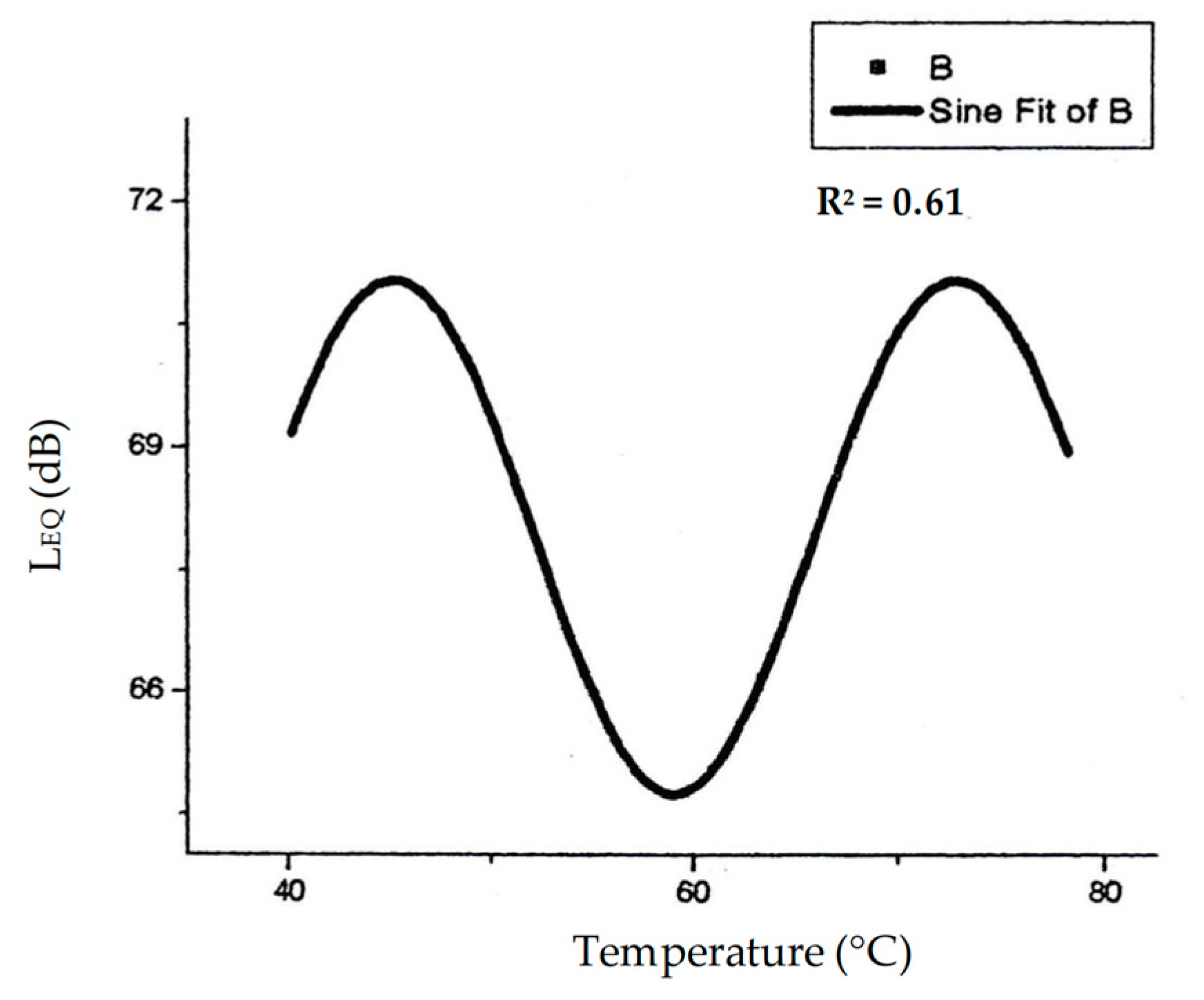
3.3. Humid Tropical Climate Influence to Noise level

Humid tropical climate has special characters which appear in high temperature and high Relative Humidity (RH), yet it has quite low difference daily temperature average. The airport is located in a northern coastal area of the city, therefore wind velocity is a significant aspect on influencing the noise level received. To observe more detail related to the correlation between climate and noise levels received in building models, based on Relative value data, the orientation angle 180 ° is chosen as the correlation model between climate and noise level, because it has the lowest sound reduction value. Therefore, in order to obtain the data on the influence of climate on noise level, rotation in the building model is not needed.

Meanwhile, the duration of the observation was carried out in the range from 06.00 AM to 07.00 PM. Based on the phenomena in the field, the predicted climate aspects greatly affecting the Noise level consist of temperature, humidity and wind speed. To obtain the synergistic data with Relative Value (R_V) and the correlation model between orientation (α) and noise level, the climate data influence were then observed in both the aircraft take-off and landing as listed in

Table 10. Climate influence to noise level.

Condition	Time	Take-off				Landing
		Leq (dB)	T °C	RH (%)	Wind (m/sec)	Leq (dB)	T °C	RH (%)	Wind (m/sec)
OS	1	70.17	24.30	95.00	0.02	65.43	30.00	65.70	1.08
	2	71.62	25.00	70.50	0.30	64.76	30.30	57.70	0.78
	3	72.18	30.90	56.70	1.20	69.77	32.50	48.10	2.00
	4	72.18	30.90	56.70	1.35	72.11	33.20	45.10	2.06
	5	68.13	34.40	45.40	1.53	71.34	34.50	41.30	3.34
	6	68.80	34.40	45.40	2.30	68.95	34.90	40.20	2.57
	7	70.26	34.50	40.20	2.70	67.10	32.00	56.50	5.00
	8	70.97	33.60	53.70	3.26	72.02	28.60	72.10	3.00
	9	67.90	31.00	63.90	3.60	70.98	28.70	76.20	2.00
	10	75.88	28.50	75.30	2.30	68.75	28.50	76.50	2.00
	11	69.86	28.60	76.80	2.00	68.11	28.10	77.20	1.60
	12	73.23	28.10	77.10	1.60	68.73	28.00	78.20	1.40
CW	1	37.95	25.50	81.00	0.07	36.48	30.80	66.30	0.04
	2	42.67	26.00	71.00	0.02	35.81	30.80	63.20	0.01
	3	43.23	31.00	60.20	0.01	40.82	32.80	50.90	0.05
	4	43.23	31.00	60.20	0.05	43.16	33.70	51.20	0.07
	5	39.18	34.90	43.90	0.01	42.39	34.80	42.40	0.05
	6	39.85	34.90	43.90	0.01	40.00	35.40	42.30	0.07
	7	41.31	35.30	42.30	0.01	38.15	32.50	59.30	0.01
	8	42.02	36.60	48.60	0.01	43.07	28.60	72.10	0.01
	9	38.95	31.00	63.90	0.01	42.03	28.70	76.20	0.01
	10	46.93	28.50	75.30	0.01	39.80	28.50	76.50	0.01
	11	40.91	28.60	76.80	0.01	39.16	28.10	77.20	0.01
	12	44.28	28.10	77.10	0.01	39.78	28.00	78.20	0.01
OW	1	67.95	25.50	80.10	0.01	63.95	25.50	79.40	0.01
	2	65,86	27.40	70.10	0.01	63.46	25.50	79.40	0.01
	3	64.00.	28.10	67.30	0.04	63.02	32.00	54.30	0.03
	4	65.84	33.50	48.20	0.03	67.71	33.40	49.90	0.01
	5	66.58	36.30	43.40	0.06	67.01	33.50	48.20	0.03
	6	66.02	37.10	39.10	0.03	67.01	36.50	42.20	0.02
	7	65.64	37.20	37.70	0.09	65.08	37.10	39.10	0.01
	8	66.58	35.80	40.40	0.12	64.98	37.10	39.40	0.02
	9	64.39	31.00	63.90	0.02	62.76	32.50	62.50	0.02
	10	65.09	28.50	75.30	0.02	66.50	28.60	72.10	0.02
	11	64.82	28.60	76.80	0.02	66.46	28.70	76.20	0.02
	12	64.91	28.10	77.10	0.02	66.48	28.50	76.50	0.02

.

Table 10 describes the data on the climate influence to noise level received in the building model at the orientation 180° as the lowest noise level receiver angle. Correlation modeling between climate aspects and noise level could be predicted to have similar pattern as those of orientation and noise level. The discussion will be explained in the discussion session.

4. Discussion

4.1. Relative Value (R_V) for Establishing Building Orientation toward Runway

Principally, the relative value (R_V) at take-off is much higher than that at landing because the noise level at take-off is much higher than that at aircraft landing. Table 3 reveals that at aircraft take-off, the building block has the lowest R_V of 0.834 and 0.703 at angle of 135° in the condition of OS-T and CW-T respectively, while the highest R_V is at an angle of 270° with 1.041 and 1.076 in condition of OS-T and CW-T respectively. This shows that the orientation of 135° was effective to reduce the aircraft noise due to the opposing position to the runway. Unfortunately, the orientation angle ranging from 270° to 330°, 0°, and 45° to 120° received much higher noise because the angles were facing the area of aircraft take-off. The highest noise level was received by the angle of 270° on its position which is perpendicular toward the peak noise at take-off. On the other hand, the orientation of 180° received much more noise coming from walls reflection of the front building block that strengthened the noise level.

In OW-T conditions (Open Window-Take-off), the lowest R_V rating is at an angle of 180° with a value of R_V 0.918, while the highest value is 330° with an R_V of 0.972. In addition, the 150° angle has a high average R_V due to the reflection factor of the wall sound in front of the configuration. Although the 330° angle in conditions outside and inside the building had a low R_V, in open window conditions it reached the highest average R_V, which was caused by a reflection factor from the front building block. While the orientation of 135° is the lowest noise level orientation for conditions outside and inside the building, in the open window condition, the orientation of 180° also has the lowest relative value (see Table 3). At the same time, other orientations toward the runway had varying values. The highest relative value is achieved by the angle of 270° for condition of outside (OS-T) and inside the building (CW-T). Table 3 shows that the highest relative value for open window conditions is achieved by an orientation angle of 330 ° because it directs to the noise peak at take-off. Similarly, the angle of 270° has noise level ranging from 0.967 to 1.076 because its position is perpendicular to the peak noise level during aircraft take-off.

In addition, in the OS-L condition (Outside of building-landing) as indicated in Table 1, the lowest R_V rating is at an angle of 135° with the highest R_V of 0.802 and the highest R_V at an angle of 270° with an R_V of 0.976. The orientation angle of 330° experiences the highest R_V because it is perpendicular to the position of the aircraft when landing. For the angles of 315° and 330°, because they were in the range of angle adjacent to 300°, then the angles were quite high on the R_V because of the reflection factor and the propagation of sound waves that form sinusoidal patterns. The relative value of the lowest sound change is achieved by an angle of 135°, and not at a 180° angle due to the reflection aspect of the sound by wall reflection of the front building configuration accelerating noise waves and strengthening the noise pressure level. In the CW-L (Closed window-landing) condition, the lowest R_V is at an angle of 135° with the highest R_V of 0.655, while the highest R_V is angle of 270° with an R_V of 0.965. The 180° angle is most effective at reducing sound levels, which can be seen from the lowest average R_V compared to any angles. The angles 300°–330° have the highest average R_V because its position is facing perpendicularly to the position of the aircraft when the peak sound at landing. Furthermore, in the measurement conditions outside the building, the lowest relative value is achieved by an angle of 135° to the runway. Unlike the OW-L conditions, the OW-L has the lowest R_V at an angle of 180° with the highest R_V of 0.903, while the highest R_V is at an angle of 330° with an R_V of 0.956.

The Table 3 shows that the orientation angle of 135° is lowest for either conditions outside or in a building, while the orientation opposite the runway (180°) has a Relative value in the window open condition, which is the most important conclusion for all conditions. On the other hand, other orientation angles have varying relative values. The highest relative value is achieved by a 270° orientation angle for conditions outside the building and inside the building, whereas the highest relative value for open window conditions is achieved by an orientation angle of 90°, which has the value of sound changes ranging from 0.697 to 0.969. These symptoms are the results of reflection and absorption of sound energy in the structure of the building block configuration.

4.2. Humid Tropical Climate Influence to Noise Level

As described in the data subheading on the climate influence to noise level received in the building model, the correlation between climate and noise level was firstly analyzed using the regression method of the 20 version SPSS software in cumulative procedure (see

Table 11. The regression of climate toward noise level at take off and landing.

Variable		Take-off		Landing
		Noise Level	Wind Speed	Noise Level	Wind Speed
Noise level	Pearson Correlation	1	0.492 **	1	0.488 **
	Sig. (2-tailed)		0.001		0.002
	N	41	41	38	38
Wind speed	Pearson Correlation	0.492 **	1	0.488 **	1
	Sig. (2-tailed)	0.001		0.002
	N	41	41	38	38

Note: ** Correlation is significant at the 0.01 level (2-tailed).

).

Further, to observe the correlation on term of establishing modeling between noise level and temperature, relative humidity (RH) as well as the wind velocity, the correlation modeling should be determined by the Origin software. The cumulative correlation can be seen in Table 11, while the correlation modeling can be illustrated in Figure 9, Figure 10, Figure 11, Figure 12, Figure 13 and Figure 14 as well as

Table 12. Correlation modeling between Temperature and Noise Level at OW-T.

Variable	Value	Standard Error
$x_c$	$11.89639$	$1.62139$
$\omega$	$5.06975$	$0.38454$
$A$	$1.4338$	$0.34164$
$L_0$	$65.6941$	$0.27528$
OW-T		$R^2=0.54$

,

Table 13. Correlation modeling between Temperature and Noise Level at OW-L.

Variable	Value	Standard Error
$x_c$	$13.80899$	$1.18945$
$\omega$	$2.72208$	$0.16983$
$A$	$-1.58536$	$0.44357$
$L_0$	$65.33293$	$0.32787$
OW-L		$R^2=0.58$

,

Table 14. Correlation modeling between Relative Humidity and Noise Level at OS-L.

Variable	Value	Standard Error
$x_c$	$-16.71270$	$5.43634$
$\omega$	$13.76808$	$0.94522$
$A$	$3.14713$	$0.72015$
$L_0$	$67.90167$	$0.55403$
OS-L		$R^2=0.61$

,

Table 15. Correlation modeling between Relative Humidity and Noise Level at OW-L.

Variable	Value	Standard Error
$x_c$	$-14.17280$	$2.08994$
$\omega$	$13.31167$	$0.37540$
$A$	$3.02166$	$0.45982$
$L_0$	$64.73870$	$0.32821$
OW-L		$R^2=0.76$

,

Table 16. Correlation modeling between Relative Humidity and Noise Level at OS-T.

Variable	Value	Standard Error
$x_c$	$12.54890$	$3.69641$
$\omega$	$0.84870$	$0.03758$
$A$	$1.02270$	$0.48807$
$L_0$	$1.97270$	$0.30437$
OS-T		$R^2=0.15$

and

Table 17. Correlation modeling between Relative Humidity and Noise Level at CW-T.

Variable	Value	Standard Error
$a$	$-0.02625$	$1.26E-04$
$b$	$0.01750$	$0.00537$
$c$	$-4.54E-04$	$1.35E-04$
CW-T		$R^2=0.61$

. Depend on the SPSS output that the temperature and humidity were less in influencing the noise level with correlation value between −0.060 to 0.020, on the other hand, the wind speed was the only aspect that significantly influenced the noise level with correlation value 0.492 to 0.488. Table 11 reveals that the wind speed influence to the noise level during take-off is the most significant of others in correlation value 0.492, while at the aircraft landing, the correlation value between noise level and wind speed is 0.488. This finding concluded that the wind speed significantly influences the noise level. Continuing on the second step on observing the correlation between noise level and climate, the origin-8 software helped to determine the R² on the climate aspects influence to the noise. As the R² is determinant coefficient means the ability of independent variable on explaining the dependent variable, the correlation modeling which was embedded with maximum R² between climate and noise can be seen in Table 12, Table 13, Table 14, Table 15, Table 16 and Table 17.

The Table 12, Table 13, Table 14, Table 15, Table 16 and Table 17 reveal the correlation modeling between climate and noise level based on the value of RR². The R² represent the correlation value between two variables. Table 12 and Table 13 describe that the temperature has a significant effect to noise level at about 0.54–0.58 maximumly. Meanwhile, the relative humidity maximumly influences the noise level at between 0.61–0.71. Table 12 and Table 13 reveal that the correlation between temperature and noise level refer to the non linier sinusoidal pattern as same as those modeling between orientation angle and noise level. A is amplitude, π/ω is constant, α is orientation angle in (°), and $\pi \ast \left(\alpha -{\alpha }_c\right)/\omega$ is phase. The high L₀ in the Table 12 indicates noise disturbance on low frequencies [7,36,37]. The determinant correlation coefficient (R²) are quite high at 0.54 and 0.58 during take-off and landing respectively because temperature is main variable on accelerating the noise wave variable in the air (see Figure 9 and Figure 10).

Like the previous correlation modeling, A is amplitude, π/ω is constant, α is orientation angle in (°), and $\pi \ast \left(\alpha -{\alpha }_c\right)/\omega$ is phase. The Table 14 and Table 15 describe that the Relative Humidity significantly influences the noise level at more than 50% among other variables. The symptoms occur due to the water vaporization which contributes noise wave absorption in the air (see Figure 11 and Figure 12). Similar to the temperature influence to the noise pressure level, in the Relative Humidity effect to noise, it is found that the L₀ is very high and over than the treeshold [7]. It is indicates that the aircraft noise is such a comprehensive noise and disturb with its low and high frequencies [36].

The most interesting is that the wind velocity is actually less in influencing the noise level refer to the Table 16. The less influence occurs due to the configuration between buildings and other mass block surrounding the ground buildings. Moreover, when the correlation modeling between wind velocity and the noise had been changed into another modeling, the influence had been increased to be 0.61 (see Figure 14). The phenomenon occur due to the sinusoidal pattern of wind direction was reflected and broken by the building mass configuration [7].

4.3. Theoretical Validation of the Correlation Modeling

Theoretical validation is carried out with the aim to prove that the correlation modeling is derived from the grand theory: inverse square law. To build a linear moving sound level equation model observed by sensoric Sound Level Meter (SLM) based on various orientation angle (α), the schematic picture in Figure 15 shows the paradigm formulation of the correlation modeling.

From Figure 15, the following mathematical equations are drawn:

$$\sin \alpha =\frac{a}{r_2}\to a=r_2\sin \alpha$$

(10)

$$\cos \alpha =\frac{r_1}{r_2}\to r_1=r_2\cos \alpha$$

(11)

On the other hand, based on inverse square law as seen in Equations (3) and (4). If the Equation (4) is substituted to the Equation (3), the formulation will be:

$$\frac{L_1}{L_2}={\left(\frac{r_2}{r_1}\right)}^2=\frac{A}{r_1^2}+\frac{B}{r_2^2}$$

(12)

where A and B are constants, and from the Equation (5), a correlation is found.

$$\frac{L_1}{L_2}=\frac{A·r_2^2}{B·r_1^2}=C·\frac{r_2^2}{r_1^2}\to C=\frac{A}{B}$$

(13)

Equation (3) is substituted to the Equations (4) and (5), it is found that:

$$\frac{L_1}{L_2}=C·\frac{r_2^2}{r_2^2·co{s}^2\alpha }=\frac{C}{co{s}^2\alpha }$$

(14)

$$L_1·co{s}^2\alpha =C·L_2$$

(15)

from the mathematical formulas, two equations applied are as follows:

$$(\mathrm{i}) si{n}^2\alpha +co{s}^2\alpha =1\to co{s}^2\alpha =1-si{n}^2\alpha$$

(16)

$$(\mathrm{ii}) si{n}^2\alpha =\frac{1}{2}-\frac{1}{2}co{s}^2\alpha$$

(17)

then, Equation (15) could be formulated as:

$$C·L_2=L_1·co{s}^2\alpha$$

(18)

$$C·L_2=L_1\left(1-si{n}^2\alpha \right)$$

(19)

$$C·L_2=L_1\left[1-\left(\frac{1}{2}-\frac{1}{2}co{s}^2\alpha \right)\right]$$

(20)

and it could be simplified as:

$$C·L_2=L_1\left[\frac{1}{2}+\frac{1}{2}co{s}^2\alpha \right]$$

(21)

On the other hand, we have the following equations:

$$co{s}^2\alpha =\sin \left[\frac{\pi }{2}-2\alpha \right]$$

(22)

$$co{s}^2\alpha =\sin \left[2\alpha -\frac{\pi }{2}\right]$$

(23)

then, it is obtained as:

$$L_2=\frac{L_1}{C}\left[\frac{1}{2}-\frac{1}{2}\sin \left(2\alpha -\frac{\pi }{2}\right)\right]$$

(24)

$$L_2=\frac{I_1}{2C}-\frac{I_1}{2C}·\sin \left(2\alpha -\frac{\pi }{2}\right)$$

(25)

$$L_2=A+B\sin \left(2\alpha -\frac{\pi }{2}\right)$$

(26)

Therefore, to determine the equation functions empirically, it must fulfill the nature of the correlation modeling in Equation (8) as:

$$L\left(\alpha \right)=C+A\sin \left(\alpha \left(\alpha -b\right)\right)$$

(27)

where C, A, α and b are searched based on observational data (empirical data). Because α and ω are together and depend on data, it is determined as:

$$\alpha =\frac{\pi }{\omega }$$

(28)

and then as a result,

$$L\left(\alpha \right)=C+A\sin \left(\frac{\pi }{\omega }\left(\alpha -b\right)\right)$$

(29)

or,

$$L=L_0+A\sin \left(\alpha \left(\alpha -b\right)\right)$$

(30)

This equation modeling is identical with the correlation modeling found by Origin-8 in this research as Equation (8). Therefore, the Equations (8) and (30) are identical, with assumption that:

$$\alpha =\frac{\pi }{\omega }$$

(31)

and

$${\alpha }_c=b$$

(32)

as that,

$$L_0=\frac{L_1}{2c}$$

(33)

with c is climatic factors such as climate and temperature. On the one hand, for the π/ω and x_c components, then in the sinusoidal pattern, it should be noted that the first peak in the highest point is assumed as S₁, while the second peak in the lowest point is assumed as S₂. Based on these assumptions, it could be determined the equations:

$$C=\frac{S_1+S_2}{2}$$

(34)

$$A=\frac{S_1-S_2}{2}$$

(35)

By understanding that the distance from the highest point to the lowest point is π, then for finding b, we should put α = 0, then:

$$L_1=C+A\sin \left[\alpha -\left(b\right)\right]$$

(36)

$$L_1=C+A\sin \left[\alpha -b\right]$$

(37)

$$\sin \left(\alpha -b\right)=\frac{L_1-C}{A}$$

(38)

$$\alpha ·b=arc·\sin \frac{L_1-C}{A}$$

(39)

$$b=arc·\sin \frac{L_1-C}{A}$$

(40)

$$b=\frac{\pi }{\omega }=\frac{22/7}{\omega }$$

(41)

$$\omega =\frac{22/7}{b}$$

(42)

If Equation (34) is substituted to the empirical data. For example, of OS-T conditions with the maximum L_eq, then the formulation will be:

$$C=\frac{74.8+90.1}{2}=82.45\to L_0$$

(43)

$$A=\frac{90.1-74.8}{2}=7.65\to A$$

(44)

understanding that $\mathit{\alpha }=\frac{\mathit{\pi }}{\mathit{\omega }}$ and $\mathit{y}\ne {\mathit{L}}_{\mathbf{1}}$, then:

$$L\left(\alpha \right)=C+A\sin \left(\frac{\pi }{\omega }\left(\alpha -b\right)\right)$$

(45)

$$L\left(\alpha \right)=82.45+7.65\sin \left(\frac{\pi }{\omega }\left(0-b\right)\right)$$

(46)

$$L\left(\alpha \right)=82.45+7.65\sin \left(-\frac{\pi b}{\omega }\right)$$

(47)

$$90.1=82.45+7.65\sin \left(-\frac{\pi b}{\omega }\right)$$

(48)

$$7.65=7.65\sin \left(-\frac{\pi b}{\omega }\right)=1$$

(49)

$$-\sin \frac{\pi b}{\omega }=1$$

(50)

$$\sin \frac{\pi b}{\omega }=-1$$

(51)

the only angle which has sin α = −1 is 3/2 π, then:

$$\frac{\pi b}{\omega }=\frac{3\pi }{2}$$

(52)

$$\frac{b}{\omega }=\frac{3}{2}$$

(53)

$$\frac{x_c}{\omega }=\frac{3}{2}$$

(54)

Therefore, it could be concluded that the mathematical modeling in this research Equation (8) is an identical derivation of the grand theory of inverse square law in Equation (3), so that the Equation (45) is identic to the Equation (8). Finally, it can be concluded that the Equation (8) is derivation of the Inverse Square Law as written in Equation (3).

4.4. Empirical Validation of the Correlation Modeling

The correlation modeling found in this study should be generalized in the case of housing around the airport. The building cluster around the airport was used as a model for empirical validation. Figure 16 shows building block having orientation angle of 66° and distance of 378.69 meters to runway. Noise level (OS-T) on the building block when the aircraft take-off is empirically measured as listed in Figure 17.

The descriptive statistic based on the empirical noise level data of the building block is shown in

Table 18. Descriptive Statistic of empirical noise level data on the 66° oriented building to runway.

Condition	N	Minimum	Maximum	Average	Standard Deviation
OS-T (66°)	20	65.10	80.50	68.04	3.96
Valid N (list wise)	20	-	-	-	-

.

Refer to the equation of correlation modeling in Table 6 for maximum OS-T where A is 7.173, α_c is 0.841, ω is 41.826 and L₀ is 83.281 dB, therefore based on the Equation (8), the noise level prediction could be calculated as:

$$\begin{gathered} L=83.381+7.173\ast \sin \left(3.14\ast \left(66-63.081/41.826\right)\right) \\ L=83.381+7.173\ast \sin \left(0.219\right) \\ L=83.381+0.027=83.405 \mathrm{dB} \end{gathered}$$

(55)

The building is located in 378.69 meter from the runway, while the modeling was established on the distance of 340.20 from the runway. Therefore, based on the Equation (6), the calculation of noise level in the distance of 378.69 to runway becomes:

$$\begin{gathered} L=L_0-10\log \left(\frac{378.69}{340.20}\right) \\ L=63.405-0.466=82.939 \mathrm{dB} \end{gathered}$$

(56)

It could be concluded that the deviation of the empirical calculation towards the measurement on site is about 1.94%. Then in this research, the equation on the 66° building block noise level when aircraft take-off has been empirically validated. Continuing on, the angle 180° building block on site (see Figure 18) when aircraft landing with the similar procedure as the previous calculation, the empirical validation, has been further discussed. Figure 10 and Figure 11 indicate the 180° oriented building block and onsite noise level measurement.

Based on the empirical measurement on noise level at the building block in Figure 19, the descriptive statistics of the empirical noise level are seen in

Table 19. Descriptive Statistics of empirical noise on the 180° oriented building to runway.

Condition	N	Minimum	Maximum	Average	Standard Deviation
OS-L (180°)	20	61.60	62.00	61.69	0.117
Valid N (listwise)	20	-	-	-	-

. Furthermore, based on Table 19 and Equations (8) the correlation modeling for the condition of the aircraft landing becomes:

$$\begin{gathered} L=58.834+3.913\ast \sin \left(3.14\ast \left(180-29.647/11.934\right)\right) \\ L=58.834+3.913\ast 0.637 \\ L=58.834+2.492=61.326 \mathrm{dB} \end{gathered}$$

(57)

The building was located 349.75 meters from the runway, while the modeling was established on the distance of 340.20 from the runway. Therefore, based on the Equation (6), the calculation of noise level in the distance of 349.75 to runway becomes:

$$\begin{array}{c}L=L_0-10\log \left(\frac{349.75}{340.20}\right)\\ L=61.326-10\log \left(\frac{349.75}{340.20}\right)\\ L=61.326-0.120=61.206 \mathrm{dB}\end{array}$$

(58)

It could be concluded that the deviation of the empirical calculation towards the measurement on site is about 1.27%. Then in this research, the equation on the 180° building block noise level during aircraft landing has been empirically validated. In so far as the angles on site are only three angles, 66°, 180° and 246°, therefore, to discuss the similar procedure for other angles of orientation,

Table 20. The empirical validation of noise level on the building block.

Aircraft Condition	Angle	On Site Measurements (dB)		Empirical Validation (dB)		Deviation
		Maximum	Average	Maximum	Average
Take-off	66°	80.50	68.04	82.94	69.36	0.0194
	180°	82.40	72.85	82.78	73.19	0.0046
	246°	82.70	73.55	83.70	74.44	0.0121
Average		81.86	71.48	83,14	72.33	0.0120
Landed	66°	67.10	60.56	66.24	60.55	0.0127
	180°	62.00	61.69	61.20	60.91	0.0127
	246°	62.20	57.26	61.66	56.76	0.0086
Average		63.76	59.83	63.03	59.51	0.0113

provides the results.

Table 20 reveals that the three angles on site have been empirically validated during aircraft take-off, the average deviation between on-site measurements and empirical validations is only about 0.0120. This value is just definitely tiny compared to the noise level received and lower than 1 dB from the greatest value of noise level measured either on site or empirical validation calculation (see Table 20).

On the other hand, during an aircraft landing, the average deviation is only 0.0113. It means that the deviation between on-site measurement and empirical validation is 0.72 dB, lower than 0.80 dB. To sum up, it could be verified that the correlation modeling could be used to predict the noise level received in building block surrounding the airport. Based on this finding, building master plan design on dwelling surrounding the airport could be performed as shown in the Figure 20. As the runway located on the northeast side of the housing cluster, The Figure 20 shows that there are no blocks facing to the runway and, instead, the blocks are oriented with an angle to runway, based on the research findings on mapping in Figure 6.

5. Conclusions

Unlike noise control themed studies in general, this research highlights building orientation mapping and the validation of noise level correlation modeling either in theoretical or empirical ways. As far as building orientation mapping is concerned, there are two important conclusions related to the orientation angles toward the runway as a noise source and critical point during an aircraft take-off and landing. For the measurement conditions of both take-off and landing, the orientation angle of 135° is the lowest in noise level value which was caused by the reflection factor and sound absorption of the building element such as, wall, roof and floor. On the other hand, for the opened window condition in both take-off and landing, the lowest Relative value was at the angle of 180°. It was caused by the configuration position towards the critical reflective angles between the building block and the block between the buildings. These symptoms occur because of the influence of the low and high frequences of noise emitted by the aircraft during take-off and landing. High frequency sound waves when the aircraft landing caused sound shadows occured due to the building mass configuration. On the other hand, low frequency sound waves caused reflection, diffraction and absorption due to the building mass configuration.

In some observations about the relationship of climate to noise level, it is found that the greatest correlation value between noise level and climate variables covering temperature, relative humidity and wind velocity are 0.58, 0.61 and 0.61 respectively. The high correlation value of wind speed to noise level proves that climate aspects, especially wind speed, have a significant effect on noise level. Continuing on this facts, during the aircraft take-off, the wind speed towards north west to the Java sea strengthens the noise level because it is in the same direction as the aircraft take-off. On the other hand, the coastal wind flowing to the mainland strengthens the noise level because it is in the direction of the plane landing. On the contrary, the land wind which flows to the coastal from the land shortens the time period of noise due to the opposite direction of the aircraft landing.

As for the validation of correlation modeling, it is concluded that the modeling is a derivation from the grand theory of inverse square law. The validation also proved that the variable of orientation angle in the housing master plan design is the most important variable beside the variable of distance and the sound pressure level. From empirical validation, it is verified that the correlation modeling could be used not only to predict the sound level received in buildings, but also to design the building orientation in the master plan of buildings surrounding the noisy airport in the city.

References

1. Harris, C.M.; Piersol, A.G. Harris’ Shock and Vibration Handbook, 5th ed.; McGRAW-HILL: New York, NY, USA, 2002. [Google Scholar]
2. Setyowati, E.; Trilistyo, H. Climate Assessment of orientation design in the housing master plan close to the airport. GSTF Int. J. Eng. Technol. 2013, 2, 158–164. [Google Scholar] [CrossRef]
3. Babisch, W.; Houthuijs, D.; Pershagen, G.; Cadum, E.; Katsouyanni, K.; Velonakis, M.; Dudley, M.L.; Marohn, H.D.; Swart, W.; Breugelmans, O.; et al. Annoyance due to aircraft noise has increased over the years—Results of the HYENA study. Environ. Int. 2009, 35, 1169–1176. [Google Scholar] [CrossRef] [PubMed]
4. Ministry of Environment, The Indonesian Government. Baku Tingkat Kebisingan (Environmental Noise Quality Standard); Indonesia, 1996; 9p.
5. Lagonigro, R.; Martori, J.C.; Apparicio, P. Environmental noise inequity in the city of Barcelona. Transp. Res. Part D Transp. Environ. 2018, 63, 309–319. [Google Scholar] [CrossRef]
6. Ganić, E.; Babić, O.; Mirjana, Č.; Stanojević, M. Air traffic assignment to reduce population noise exposure using activity-based approach. Transp. Res. 2018, 63, 58–71. [Google Scholar] [CrossRef]
7. Caniato, M.; Bettarello, F.; Schmid, C.; Fausti, P. Assessment criterion for indoor noise disturbance in the presence of low frequency sources. Appl. Acoust. 2016, 113, 22–33. [Google Scholar] [CrossRef] [Green Version]
8. Setyowati, E.; Sadwikasari, A.F. Building materials composition influence to Sound Transmission Loss (STL) reduction. Adv. Mater. Res. 2013, 789, 242–247. [Google Scholar] [CrossRef]
9. Setyowati, E. Algorythm Evolution of new environmental acoustic theory on housing masterplan design. Int. J. Eng. Technol. 2013, 13, 49–58. [Google Scholar]
10. Ozkurt, N.; Hamamci, S.F.; Sari, D. Estimation of airport noise impacts on public health. A case study of Izmir Adnan Menderes Airport. Transp. Res. Part D Transp. Environ. 2015, 36, 152–159. [Google Scholar] [CrossRef]
11. Licitra, G.; Gagliardi, P.; Fredianelli, L.; Simonetti, D. Noise mitigation action plan of Pisa civil and military airport and its effects on people exposure. Appl. Acoust. 2014, 84, 25–36. [Google Scholar] [CrossRef]
12. Lawton, R.N.; Fujiwara, D. Living with aircraft noise: Airport proximity, aviation noise and subjective wellbeing in England. Transp. Res. Part D Transp. Environ. 2016, 42, 104–118. [Google Scholar] [CrossRef]
13. Lambert, J.; Champelovier, P.; Blanchet, R.; Lavandier, C.; Terroir, J.; Márki, F.; Griefahn, B.; Iemma, U.; Janssens, K.; Bisping, R. Human response to simulated airport noise scenarios in home-like environments. Appl. Acoust. 2015, 90, 116–125. [Google Scholar] [CrossRef]
14. Krunic, N.; Nenkovic, M. The impact of airport noise as part of a Strategic Environmental Assessment, case study: The Tivat (Montenegro) Airport expansion plan. Transp. Res. 2016, 49, 271–279. [Google Scholar]
15. Janssen, S.A.; Centen, M.R.; Vos, H.; Van Kamp, I. The effect of the number of aircraft noise events on sleep quality. Appl. Acoust. 2014, 84, 9–16. [Google Scholar] [CrossRef]
16. Camara, T.; Kamsu-Foguem, B.; Diourte, B.; Faye, J.P.; Hamadoun, O. Management of acoustic risks for buildings near airports. Ecol. Inform. 2018, 44, 43–56. [Google Scholar] [CrossRef]
17. Gagliardi, P.; Teti, L.; Licitra, G. A statistical evaluation on flight operational characteristics affecting aircraft noise during take-off. Appl. Acoust. 2018, 134, 8–15. [Google Scholar] [CrossRef]
18. Ignaccolo, M. Environmental capacity: Noise pollution at Catania-Fontanarossa international airport. J. Air Transp. Manag. 2000, 6, 191–199. [Google Scholar] [CrossRef]
19. Sahai, A.K.; Snellen, M.; Simons, D.G. Objective quantification of perceived differences between measured and synthesized aircraft sounds. Aerosp. Sci. Technol. 2018, 72, 25–35. [Google Scholar] [CrossRef]
20. Schäffer, B.; Plüss, S.; Thomann, G. Estimating the model-specific uncertainty of aircraft noise calculations. Appl. Acoust. 2014, 84, 58–72. [Google Scholar] [CrossRef]
21. Lu, C. Combining a theoretical approach and practical considerations for establishing aircraft noise charge schemes. Appl. Acoust. 2014, 84, 17–24. [Google Scholar] [CrossRef]
22. Aparecida, T.; Ghislain, J.; Maldonado, F. Analysis of airport noise through L Aeq noise metrics. J. Air Transp. Manag. 2014, 37, 5–9. [Google Scholar]
23. Xie, H.; Li, H.; Kang, J. The characteristics and control strategies of aircraft noise in China. Appl. Acoust. 2014, 84, 47–57. [Google Scholar] [CrossRef] [Green Version]
24. Pàmies, T.; Romeu, J.; Genescà, M.; Arcos, R. Active control of aircraft fly-over sound transmission through an open window. Appl. Acoust. 2014, 84, 1–6. [Google Scholar] [CrossRef]
25. Ku, H.; Kim, H. Acoustic insulation performance of improved airtight windows. Constr. Build. Mater. 2015, 93, 542–550. [Google Scholar]
26. Suárez, E.; Barros, J.L. Traffic noise mapping of the city of Santiago de Chile. Sci. Total Environ. 2014, 466–467, 539–546. [Google Scholar] [CrossRef] [PubMed]
27. Cai, M.; Zou, J.; Xie, J.; Ma, X. Road traffic noise mapping in Guangzhou using GIS and GPS. Appl. Acoust. 2015, 87, 94–102. [Google Scholar] [CrossRef]
28. Tsai, K.; Lin, M.; Chen, Y. Noise mapping in urban environments: A Taiwan study. Appl. Acoust. 2009, 70, 964–972. [Google Scholar] [CrossRef]
29. Ko, J.H.; Chang, S.I.; Lee, B.C. Noise impact assessment by utilizing noise map and GIS: A case study in the city of Chungju, Republic of Korea. Appl. Acoust. 2011, 72, 544–550. [Google Scholar] [CrossRef]
30. Vogiatzis, K.; Remy, N. From environmental noise abatement to soundscape creation through strategic noise mapping in medium urban agglomerations in South Europe. Sci. Total Environ. 2014, 482–483, 420–431. [Google Scholar] [CrossRef]
31. Dintrans, A.; Préndez, M. A method of assessing measures to reduce road traffic noise: A case study in Santiago, Chile. Appl. Acoust. 2013, 74, 1486–1491. [Google Scholar] [CrossRef]
32. Bastián-Monarca, N.A.; Suárez, E.; Arenas, J.P. Assessment of methods for simplified traffic noise mapping of small cities: Casework of the city of Valdivia, Chile. Sci. Total Environ. 2016, 550, 439–448. [Google Scholar] [CrossRef]
33. Duta Citra Consultant. Final Report: Building and Environment Spatial Planning (RTBL) in Ahmad Yani Airport Area Semarang; Semarang, Indonesia, 2005. [Google Scholar]
34. International Organization for Standardization. ISO 1996-1: 2016: Acoustics—Description, Measurement and Assessment of Environmental Noise—Part 1: Basic Quantities and Assessment Procedures; International Organization for Standardization: Geneva, Switzerland, 2016; 11p, Available online: https://www.sis.se/api/document/preview/920252/ (accessed on 19 January 2019).
35. Filippone, A. Aircraft noise prediction. Prog. Aerosp. Sci. 2014, 68, 27–63. [Google Scholar] [CrossRef]
36. Persson-Waye, K.; Bjorkman, M.; Rylander, R. Loudness, annoyance and dBA in evaluating low frequency sounds. J. Low Freq. Noise Vib. Act. Control 1990, 9, 32–45. [Google Scholar] [CrossRef]
37. Sahlgrenska Academy. Effects of Low Frequency Noise and Vibrations: Environmental and Occupational Perspectives; Göteborg University: Göteborg, Sweden, 2011; pp. 240–253. [Google Scholar]
Figure 1. Noise Mapping in Achmad Yani International Airport in Semarang city [33].
Buildings 09 00027 g001
Figure 2. Location of the housing cluster near the runway.
Buildings 09 00027 g002
Figure 3. Measurement procedure with building model. (a) building model with α facing to runway; (b) building model with rotated α.
Buildings 09 00027 g003
Figure 4. Placement of building model in the location near the runway; (a) control building model; (b) building block model was rotatable on its axis.
Buildings 09 00027 g004
Figure 5. Reflection and absorption in orientation 135° and 180°.
Buildings 09 00027 g005
Figure 6. Building Orientation mapping to runway.
Buildings 09 00027 g006
Figure 7. Maximum Leq at OS-T [9].
Buildings 09 00027 g007
Figure 8. Average Leq at OW-L [9].
Buildings 09 00027 g008
Figure 9. Correlation modeling between Temperature and Noise Level at OW-T.
Buildings 09 00027 g009
Figure 10. Correlation modeling between Temperature and Noise Level at OW-L.
Buildings 09 00027 g010
Figure 11. Correlation modeling between Relative Humidity and Noise Level at OS-L.
Buildings 09 00027 g011
Figure 12. Correlation modeling between Relative Humidity and Noise Level at OW-L.
Buildings 09 00027 g012
Figure 13. Correlation modeling between Relative Humidity and Noise Level at OS-T.
Buildings 09 00027 g013
Figure 14. Correlation modeling between Relative Humidity and Noise Level at CW-T.
Buildings 09 00027 g014
Figure 15. Building orientation angle toward runway.
Buildings 09 00027 g015
Figure 16. The 66° oriented building block toward runway.
Buildings 09 00027 g016
Figure 17. Empirical Noise level (OS-T) of 66° oriented building toward runway.
Buildings 09 00027 g017
Figure 18. The 180° oriented building block toward runway.
Buildings 09 00027 g018
Figure 19. Empirical noise level (OS-L) of 180° oriented building toward runway.
Buildings 09 00027 g019
Figure 20. (a) Dwelling layout design in residence area closed to the airport; (b) Key plan.
Buildings 09 00027 g020