Article

Duration and Labor Resource Optimization for Construction Projects—A Conditional-Value-at-Risk-Based Analysis

1
School of Civil Engineering, Qingdao University of Technology, Qingdao 266033, China
2
Department of Civil and Environmental Engineering, Syracuse University, Syracuse, NY 13244, USA
3
Department of Systems Engineering and Engineering Management, University of North Carolina at Charlotte, Charlotte, NC 28223, USA
4
New Huayou Construction Engineering Group Co., Ltd., Qingdao 266033, China
*
Author to whom correspondence should be addressed.
Buildings 2024, 14(2), 553; https://doi.org/10.3390/buildings14020553
Submission received: 19 December 2023 / Revised: 26 January 2024 / Accepted: 5 February 2024 / Published: 19 February 2024
(This article belongs to the Special Issue Construction Scheduling, Quality and Risk Management)

Abstract

:
The complexity and uncertainty of construction projects contribute to low efficiency in the construction industry. This research applied the Takt-time planning method to optimize the construction working process, and proposed a risk control framework based on Value at Risk (VaR) and Conditional Value at Risk (CVaR) approaches to explore and predict a project schedule and cost performance under different scenarios. This research selected a high-rise residential building project for a case study and collected 1672 productivity data samples. Arena Simulation models were established based on 90 combinations of labor assignments to assess Takt-time planning strategies’ impact on project performance in four scenarios. The VaR and CVaR evaluations at 75% and 90% confidence levels were compared to balance project benefits and risks. Without any overtime or additional workers, this research found a Takt-time planning method that can reduce the project duration by 20.2% and labor costs by 2.1% at the same time, using a labor assignment of 12 bar placers, 12 carpenters, and 5 pipefitters. The findings can assist construction managers to achieve a shorter duration, reduced cost, and safer work environment, which will be very effective and beneficial to improve project overall performance.

1. Introduction

Construction projects are often characterized by complexity and variability, making project management a very difficult task in the construction industry and leading to inefficiencies in the whole process [1,2]. Project managers need to spend a lot of time and effort to keep track of various information about the project. Therefore, an effective and efficient method to help them perform this work is very important. In construction planning, each piece of information contains unique uncertainties, and such uncertainties make project decisions risky [3]. At present, there is a lack of a decision-making mechanism in the field of building construction management that takes into account the subjective tendency of the managers and the objective situation of the project. Therefore, the objectives of this research are to (1) establish a workflow simulation to explore how various Takt-time planning strategies impact project duration and cost performance; (2) develop a risk control framework based on Value at Risk (VaR) and Conditional Value at Risk (CvaR) approaches to quantify the risks associated with different construction scenarios, balancing subjective tolerance levels and objective project performance; and (3) develop recommendations for optimal resource allocation to enhance the work efficiency and risk control.

2. Literature Review

2.1. Takt-Time Planning Method

The construction industry has long attempted to benefit from manufacturing technologies to improve productivity. However, in most of the current practice, the construction sites heavily rely on managers’ experience to coordinate the scheduling. Faghihi et al. compared existing studies and found that the research on optimizing construction scheduling mainly focuses on the temporal aspects of the project schedule [4]. However, the importance of working space availability at an assigned location tends to be ignored [5,6,7,8,9].
The word Takt in German means beats [10]. The first mention of Takt production in construction dates back to the time the Empire State Building was built in the 1930s, when Takt-time was called a “pacemaker” [11,12]. A more systematic use of Takt-time emerged in the early 2010s via Greg Howell, Mario Fiallo, Iris Tommelein, etc. [12]. Takt-time is a manufacture term used to describe the rate at which a good needs to be produced to meet customer demand [11]. It can be interpreted as the speed at which customers require products. Takt-time = (Net Time Available for Production)/(Customer’s Daily Demand) [12]. Takt-time planning is carried out by first determining preliminary Takt and planning the work zones, then optimizing labor, space, and duration assignments to enhance a smooth flow of workers entering and leaving a workspace at a fixed time interval (Takt), one crew at a time. The uniqueness of Takt-time planning is that it assigns only one crew to work in a specific space within a Takt, minimizing the chance of overcrowding or work waiting for workers to protect productivity [12,13]. The Takt-time planning method ensures continuity and stability in the execution of work and defines clear handoffs between operators to facilitate coordination and control [14,15]. Software such as Tactplan 1.0 and inTakt 1.0 was developed to facilitate Takt-time planning.
Lerche et al. applied Takt-time scheduling to the assembly of six towers in an offshore project, and the intervention reduced the time per tower module by nine days and the loading interval by 3.6 days, which reduced wastage and uncertainty in the construction schedule [13]. Kimmo et al. applied Takt-time scheduling to a project of about 200 units of a refurbished apartment building, and the rationalization of the Takt-time and the division of areas allowed the building to be delivered on time, and pointed out that Takt production must be planned [16]. Janosch et al. developed a methodology for designing Takt planning and Takt control systems based on the Takt-time scheduling method, which was applied to a large construction project, bridging the various construction phases and reducing the construction time from the original 11 months to 5 months [17]. Current Takt-time planning tools were not designed to reflect the dynamic interaction between duration and manpower allocation. Therefore, this research developed simulation models using empirical productivity data to help construction managers thoroughly understand the dynamics and visualize the potential risks.

2.2. Arena Computer Simulation

Construction projects are complex and dynamic in nature, and with the increasing size and complexity of construction projects, most of the traditional manual quantitative analysis methods are not able to effectively and accurately capture the project productivity performance indicators [18]. Arena Simulation software is a widely used and accepted simulation tool in the field of industrial technology [19,20]. Durdu et al. developed a simulation model of automotive production using Arena, performed a system analysis to find the bottlenecks in the production process, and proposed a facility layout plan to achieve the goals of eliminating delays. The research reduced total production time and improved productivity [21]. Li et al. proposed a new benchmark to assess the benefit–cost ratio of regional traffic volume based on the advantages of Arena Simulation with high data availability and fast simulation speed to customize the incident scenarios in highway service patrols, and simulate and evaluate the benefit–cost ratio under different scenarios [22]. In the field of construction engineering, Chen et al. redesigned the 16 steps of prefabricated constructed buildings using the Judgment, Processing, and Transfer modules of the Arena, which resulted in an overall savings of 24% in production time and a reduction in space requirements, idle time, and resource conflicts in assembly operations [19]. He et al. applied Arena Simulation to 17 activities in a high-rise residential building to simulate 89 workforce and 2 fast-follow-up levels to explore the impact of scenario changes on the project [23]. This research applied Arena Simulation 15.1 to establish the simulation model. Developed by Rockwell Software, Arena Simulation version 16 is computer software for process flow simulation modeling.
In construction research, simulation has been used as a decision support tool to quantitatively analyze activity operations and project performance [24,25]. In this paper, the Arena Simulation model was applied to repetitive construction activities in order to optimize the construction schedule. In contrast to other models, the simulation moves forward only when the external events arrive, rather than using a uniform time step. Therefore, the Arena model is capable of simulating more realistic operations [22,26].

2.3. VaR- and CVaR-Based Risk Assessment

Risk management and risk metrics have their origins in the financial and insurance industries [27]. In 1999, the concept of VaR was introduced to quantify significant losses associated with the probability of occurrence in the measurement of financial market risk and regulatory capital in accordance with the Basel Accord [28,29]. VaR is based on mathematical methods to quantify risk and is a typical risk measure that plays a key role in regulation, forecasting, etc. [30,31,32]. As an extension to the concept of VaR, the CVaR is the conditional mean of asset loss over VaR at the corresponding confidence level [33,34]. Compared to other assessment methods, the VaR concept is simple and intuitive, easy to calculate, and easy to implement; CVaR is a downside risk-focused, quartile-based risk metric, implying that the risk loss is determined by the right-tailed quartile. VaR and CVaR are evaluated considering the subjective preference and a large amount of distribution data. Decision making can be assisted by adjusting the preference, i.e., the confidence level in this paper, to predict the outcomes under different ideas, and also to give remedies for unfavorable situations that have already occurred [35,36]. Alejandro et al. conducted VaR and CVaR analyses for finance (optimal investment) and insurance (optimal reinsurance) to prove their practical effectiveness [37]. Harry utilized VaR and CVaR to find the optimal trade-off between return and risk in an application that assumes a financial market consisting of a bank account and a stock [38]. Hu et al. developed a risk control model for water allocation and economic loss based on the integration of the CVaR and Gini coefficient, which was verified during the construction for the Qujiang River Basin [39].
Construction projects are usually characterized by a high degree of complexity [40,41]. Construction project management should be both reliable and resilient, dealing with high probability events with low impact and guarding against events that have a considerable impact on the outcome [42,43]. Franco et al. introduced VaR to quantitatively check the level of risk in bidding investment decisions and validated it in co-generation power plant projects to help balance the overall project portfolio of engineering and contracting firms [44]. Alireza et al. applied VaR to the calculation of escalation factors to realize the preparation of budgets for construction projects, which reduces the prevalence of over-budget risk [45]. Decisions in construction management are often made in complex, dynamic, and uncertain environments, making effective planning and risk assessment particularly important [46]. Mohsen et al. proposed the design planning of a hybrid reverse logistics network based on CVaR, which solved the network design problem of recovering the product and investment rate under uncertainty [47]. He et al. applied VaR and CVaR to 267 construction scenarios of high-rise residential buildings to establish a risk control framework to assess project risks [48]. In recent years, although research on topics related to risk management and risk metrics has spread across different industrial fields [49], the research application of VaR and CVaR in the construction field is still relatively small; therefore, in this paper, VaR and CVaR approaches were used to synergistically analyze the uncertainty of construction scenarios and to predict the probability of the occurrence of various events. The goal was to evaluate the resilience and robustness of different decisions of the project, and to help the project managers to look for the objects of maximizing the rewards and minimizing the risks in different scenarios [50].

3. Research Method

As illustrated in Figure 1, the research steps of this paper are as follows: (1) based on the case study, apply the Takt-time planning method to gradually optimize the promotion of resource allocation and optimize the construction scheduling process; (2) based on the collected productivity data, set up Arena Simulation to analyze the interaction between labor, duration, and cost under different scenarios; (3) organize the simulation data for probability function fitting, apply VaR and CVaR to quantify the risk value of different construction scenarios, and customize the construction strategy based on the subjective risk tolerance of the manager.

3.1. Data Collection

This research collected empirical production data by recording the detailed activity operations at one or two person–crew levels on an hourly basis, and conducting in-depth interviews with the workers and managers. The data were organized at the close of business each day, and Table 1 shows an example of the data collection form for one activity. Figure 2 shows the corresponding construction activity critical path (CPM) diagrams that were determined after the aggregation of activities from multiple repetitive criteria layers. After data were collected, the data were organized into tables by activity type and location number to calculate productivity (activity duration/quantity of the work). A statistical analysis was performed to identify the productivity distribution type and parameters for each activity. Appendix A and Appendix B show examples for productivity calculation and distribution fitting.

3.2. Apply Takt-Time Optimization

One of the main contributions of this research is to use a real project to demonstrate how to adjust the construction process, and delineate the workflow to provide a large number of feasible Takt-time planning alternatives and the subsequential cost and duration. Appendix C shows the activity duration analysis results based on the empirical production data collected from the project.
The Takt-time planning method reprogramming the number of workers and working hours for the major trades to ensure the workflow follows a certain rhythm. By consulting with the appropriate management personnel, some adjacent activities can be performed in parallel by setting the overlap percentage on the basis of the original sequence, i.e., fast-track. For example, in this research, tying vertical column bars allows for a fast-track of 50%, indicating that tying vertical column bars can start after the previous activity of column straight reinforcement bar extension has completed 50% for the whole floor. In order to accelerate the project effectively, projects often use the fast-track technique to shorten the duration [6]. In this regard, this paper accordingly modeled non-fast-track and fast-track, and designed the overlap ratio of sequential activities.
The delineation of the construction area for the activities is re-planning the working area of different trades so that only one type of trade is operating in a single area per unit Takt. For example, at the beginning of the new floor, scaffolders were building the outer frame, carpenters were matching the vertical formwork, bar placers were tying the column rebars, pipefitters installed the wall wiring pipe. At the same time, there were workers going back and forth to different floors to transport materials. During this time, there were more than 30 workers sharing the same floor. They can run into each other’s traffic paths. Therefore, based on the work method and pattern, bar placers and scaffolders were divided into staggered areas, while limiting the time of entry of pipefitters and carpenters, so as to reduce the interruption of working areas by various trades.

3.3. Arena Simulation

The simulation model of the construction activities was developed by formulating the corresponding logical relationship judgments according to the CPM diagram. Figure 3 shows the operation logic diagram adopted by the model, which is divided into 3 parts—(1) yellow section: responsible for data input/output and constructing the construction scenario; (2) orange section: the decision procedure of not setting up fast-tracking or not allowing the fast-tracking process; and (3) blue section: the decision procedure of allowing the fast-tracking process under the fast-follow-up model. Appendix D shows an example of the Arena modeling. Equation (1) is used to calculate the duration in the model:
D = W C × P
where D is the duration of an activity, and P, W, and C correspond to the workload, productivity, and number of workers, respectively. For instance, if the quantity of P for tying beam reinforcing bars is 246.14 m, C is 12 workers, and W is 15 min/m (generated by a productivity function of 2 + LOGN(12.9,10.3)); D is 308 min = 15 × 246.14/12, equivalent to 5.13 h.
The modules used for each activity are (1) create; (2) assign; (3) process; (4) read/write; (5) dispose; (6) decide and delay: to determine whether the previous activity is complete or not, and to decide whether to delay its successor. Module (6) only exists for activities that have predecessors.
The production rates used in the assign module fall into two main categories. One is a continuous probability distribution function generated by fitting multiple sets of empirical productivity data, e.g., tying column bars, tying beam bars; the others used discreet discrete probability density functions, e.g., installing formwork, installing wiring and a conduit.
According to the schedule and work pattern of the project, one Takt was determined to be 5 h. In the case that an activity has a duration of less than one hour, the model deferred to overtime to complete the activity. An example is if an activity needs 10.5 h to complete. Two Takts are 10 h. Instead of having a third Takt totally devoted for the remaining 0.5 h, the model used overtime of 0.5 to complete the activity.

3.4. VaR and CVaR Evaluation Analysis

The results of 4500 permutations of construction arrangements were simulated using the Arena model. In order to effectively assist managers to select the optimal solution among these combinations according to their own project conditions and preference, this research adopted the VaR and CVaR methods for risk assessment to provide decision support for construction managers. The VaR and CVaR methods can clearly select the optimal solution among a large number of alternatives and ensure that the solution meets the managers’ preference as well as the objective constraints of the site.
VaR calculates the maximum loss expected at a given significance level, which in this research can be interpreted as the latest time to finish at a given confidence level. For example, a VaR of 20 days for α = 90% implies that the probability of not finishing in 20 days is limited to 10% [51]. The confidence level α represents the decision maker’s risk tolerance level.
Equation (2) was used to evaluate VaR. Let a series of events obey a probability distribution X, whose probability density function (PDF), i.e., f(x), and cumulative distribution function (CDF) can be calculated. Let the VaR value of X be at confidence level α, i.e., it should be satisfied:
ψ f ( x ) d x = α
Assuming the relative duration of the PDF for f(x), project managers aim to ascertain the completion time for α = 90% of the project, wherein the CDF equals F(x) = 90%. Substituting this into Equation (2) yields a result of 0.700, which is then translated into a VaR of 90% as VaR(0.9) = 70.0%. In conjunction with Equation (2), VaR can be understood as the maximum upper bound in the manager’s given confidence level α or acceptable range. VaR ignores the 100 (1 − α)% out-of-acceptance range scenario and focuses on the α% best-case scenario only.
The concept of VaR is simple and can be quickly applied to find the maximum upper limit of the acceptable range. But VaR itself has some drawbacks. As a discontinuous risk measure [31], the VaR function is non-convex and not sub-additive, so when the extent of loss exceeds the confidence level, i.e., α, the VaR measure does not provide any indication of the severity of loss beyond the confidence level [27,52].
Instead, CVaR allows for the measurement of risk beyond the confidence level scenario. CVaR, as a risk metric mechanism that extends VaR, will take into account these extreme events in order to minimize their impact, allowing for risk assessment in the most unlikely scenarios (beyond the confidence level) [53]. Unlike VaR, CVaR is a consistent risk measure and a convex function with sub-additivity [52]. From a computational point of view, CVaR usually does not significantly increase the complexity of the optimization model [30,37]. From a practical point of view, CVaR takes tail extremes into account, effectively metrics the tails to obtain a globally optimal solution, and provides a relatively conservative risk metric value with higher security and stability [52,53,54,55].
C V a R α ( x ) = 1 1 α α 1 V a R t ( x ) d t
Equation (3) is calculated based on Equation (2), and the example where α = 90% is still employed here. Initially, the integral of VaRₜ(x) within the range of 0.9 to 1 is computed, followed by multiplying the integration result of 0.0862 by the weighted average of 1/0.1 to obtain CVaR(0.9), which equals 86.2%. Equation (3) was used to calculate CVaR. In Equation (3), CVaR represents the expected loss beyond the accepted range. According to Equation (3), CVaR can be interpreted as an integral from α to 1 that calculates the expected time for all extremes that exceed the confidence level α, and then divides the result by the percentage of extremes (1 − α). Thus, CVaR reflects the conditional expected value of the extremes, or the average loss in excess of the acceptable level of risk. Compared to VaR, CVaR assesses risk from a more conservative perspective and provides more robust optimization.
A total of 4500 sets of data from 50 simulations of 90 labor combinations of the selected model were simulated and the function images were fitted. Assuming that the minimum value of the total duration in model (1) is 50 h and the maximum value is 90 h, which is normalized to 0–1 for the fairness measure, the actual duration is transformed into the corresponding percentile values using Equation (4) [52]. A histogram plot was developed in steps of 2.5% and the probability density function was fitted using the great likelihood estimation method. Combined with the subjective risk tolerance of the project manager, the relative duration under the confidence level α was calculated using VaR Equation (2), and the optimal solution for the extreme case beyond the acceptable situation was calculated using Equation (3). At the same time, if the confidence level α corresponding to the relative duration is known, the maximum duration corresponding to this confidence level can be derived inversely [51]. For example, the minimum value of the duration of the simulation is xmin = 30 h and the maximum value is xmax = 60 h; now, the relative duration at x = 42 h is required, which can be obtained by substituting into Equation (4) as 40%.
x % = x x min x max x min × 100 %

4. Case Studies

The case study is a high-rise residential project under construction in Qingdao with a cast-in-place shear wall structure, Building #7, including 3 floors underground and 22 floors above-ground, with a total floor area of 11,156 square meters. The standard floor is an approximate rectangle, with a length of 34 m, a width of 15.7 m, and a single-floor area of 534 m2. The project started in February 2022. The building entered the main structure construction phase in April. When data collection commenced in July, the building was in the initial stages of constructing the 13th floor. The entire main structure was anticipated to be completed by September 2022.

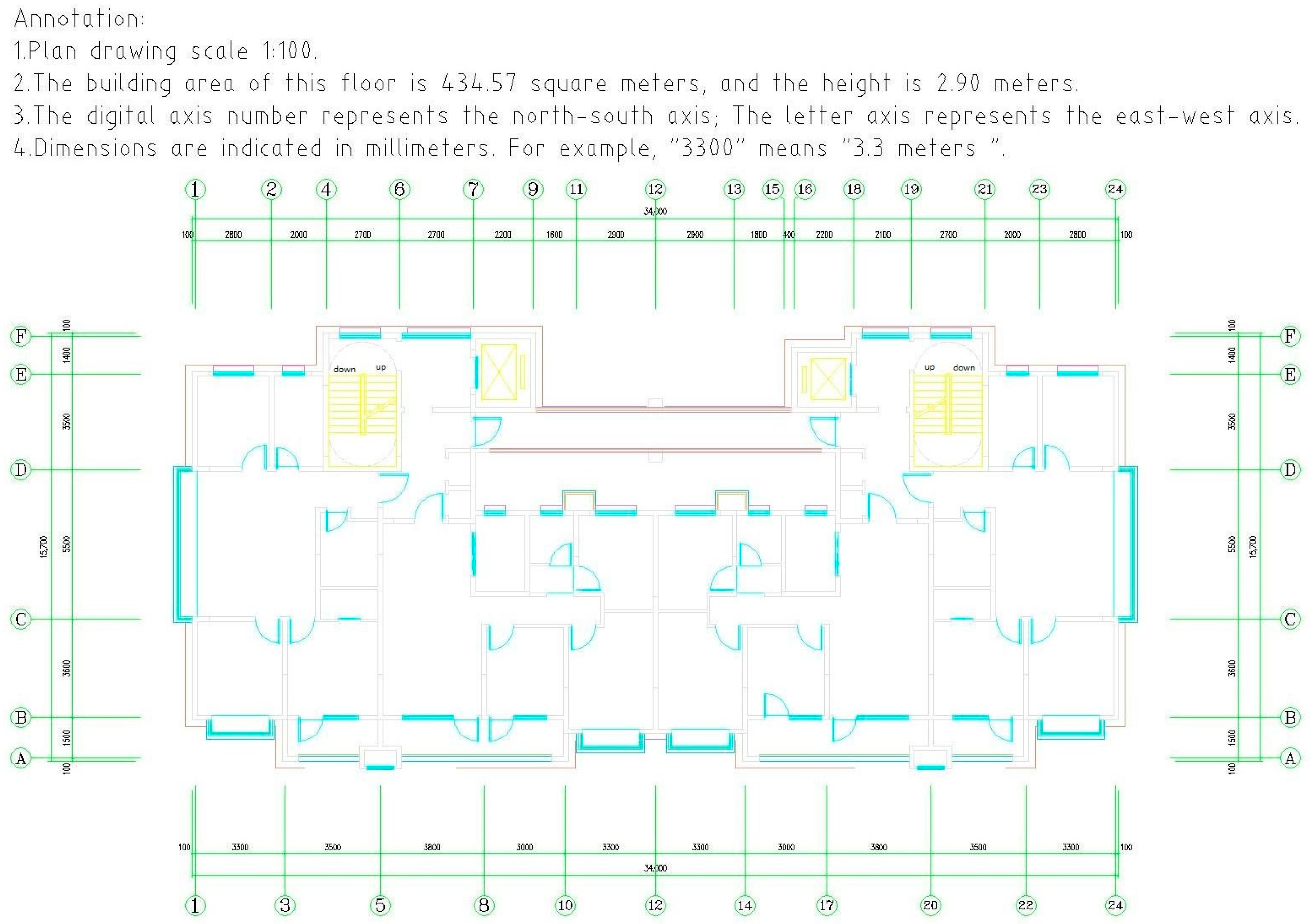
4.1. Preliminary Work

Figure 4 shows the standard floor construction plan, and the project has standardized floors from the 2nd to the 21st floor. The structural design and construction methods are identical for each floor. Based on the experience of the site managers, the production data above the 19th floor became more stable and representative. This is because the initial and end construction may be affected by the effect of start-up in the early stage and finishing-up at a later stage. Therefore, this study collected data from the 14th to 17th floors. Two authors stayed at the jobsite for the entire data collection period, 37 workdays from July to August 2022. They observed and recorded the start and finish of each crew (typically one or two workers) for each activity from the beginning to the end of working time every day. As shown in Table 1, they recorded the date, location, start and finish time, and workspace of each crew for each activity. For example, two workers erected column rebar on 15 July from 8:30–9:15 a.m. between the designated column numbers in the structural design. In total, the research team collected 1672 pieces of productivity data. The data were updated in a shared folder and checked daily by the research group and compiled in a spreadsheet for a further analysis.
Eighteen construction activities were identified after four layers of repetitive criteria layer aggregation, and the corresponding CPM diagrams are shown in Figure 2, with different colors corresponding to different work types. On average, it takes 78 h per layer. Figure 5 includes site photos of construction activities.
According to the site conditions, the site workers can be categorized into carpenters, bar placers, pipefitters, concrete workers, and scaffolders. Carpenters are roughly equally subcontracted to four groups according to the floor plan, and the rest of the laborers are day laborers and team workers. Carpenters were divided into four groups from left to right, and there are four, two, three, and two workers per group. They worked 7 days a week for an average of 10 h per day, from 6:00 a.m.–11:00 a.m., and from 1:00 p.m.–6:00 p.m. The work of other trades was relatively unstable depending on the completion of their predecessors, and interruption from the adjacent buildings. In general, they followed the same work hours as the ones of the carpentry.

4.2. Make Takt-Time Adjustments

The optimization process of the Takt-time planning method includes the following three steps: (1) Determine the number of people working—according to the site’s working conditions and consulting management personnel, the number of workers assigned for the bar placing activity was 11, 12, 13, 14, 15, and 16; carpentry was 10, 11, 12, 13, and 14; pipefitting was 4, 5, and 6; and the permutations and combinations were carried out to form a total of 6 × 5 × 3 = 90. For example, the combination 12, 10, and 4 indicates that there are 12 bar placers, 10 carpenters, and 4 pipefitters. The numbers of scaffolders, concrete workers, and bar placers were fixed and there is no work surface competition with other types of work in the actual operation. Therefore, this research did not adjust it. (2) Delineation of working hours—because carpentry is the key activity on the critical path, the working hours for the construction site were standardized from 6:00 to 11:00 and 13:00 to 18:00, using the working hours of carpenters as the benchmark. Accordingly, a Takt of 5 h was used. If an activity took less than 5 h, it was counted as 5 h. (3) Delineation of the work area—the building is a four-family residential building with symmetrical structure except for the elevator part, so the floor plan was divided into two areas: the left H and the right B as shown in Figure 6.

4.3. Generate Simulation Data

All available data were imported into Arena’s built-in Input Analyzer for function fitting, and productivity distribution functions were developed and used for model simulation. Random samples from the productivity distribution function were used as productivity inputs for each simulation.
Depending on the actual situation, some of the activities can be fast-tracked. Therefore, four sub-models were created by adjusting the Takt-time planning method: (1) no-fast-track and Takt = 5; (2) no-fast-track and Takt = 2.5; (3) 50% fast-track and Takt = 2.5; and (4) H-B area delineated, 50% fast-track, and Takt = 2.5. A detailed model is attached as Appendix D. Each sub-model simulates the aforementioned 90 labor combinations in the Arena model, respectively. Each combination was run 50 times and a total of 18,000 sets of outputs were produced. The details of research steps can be found in Appendix E.

5. Results and Discussion

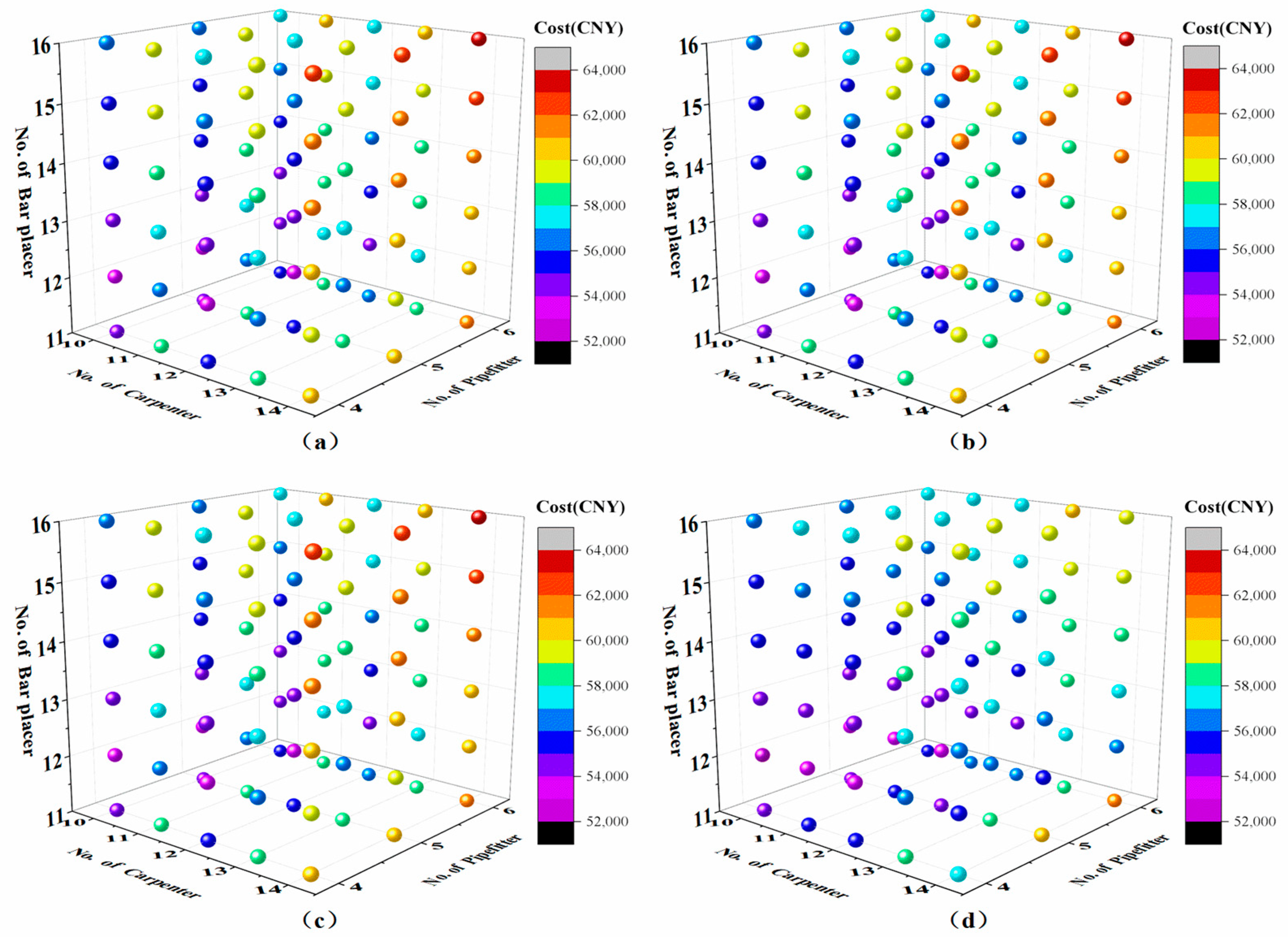
5.1. Optimization of Model and Workforce Combinations at Takt-Time

Figure 7 and Figure 8 show the results of the simulation for project duration and cost. Each color mapping chart corresponds to a model constructed in Arena, where the x-axis represents the number of carpenters, the y-axis represents the pipefitters, and the z-axis represents the bar placers. The coordinate points signify the corresponding simulation data.

5.1.1. Vertical Comparison: Different Models with the Same Labor Combination

The results of the comparison of the durations required for the same labor combination are shown in Table 2. The comparison of Figure 7 and Table 2 shows that shortening Takt = 5 to Takt = 2.5 results in a 3.2% reduction in the duration. By adjusting smaller Takt changes, we found more gap time and repetitive work. But there was no significant decrease in the duration found. The most obvious reduction in duration was found when fast-tracking was used. The goal of Takt production is to identify repetitive processes in production and balance them, and more repetitive work can be found by dividing smaller areas [17].
After continuously improving the Takt-time approach using the four models, the research found smaller Takt variations, a more compact process, smaller zones, and more gap time. The floor duration was 20.2% shorter than the actual duration of the project and uncertainty in man hours was also reduced. Accompanied by adequate batch sizes, Takt production can be considered to radically reduce the duration of production [56].
The reduction in project duration often requires additional costs [6]. This paper reduces indirect costs while avoiding additional labor costs by setting a Takt of 5 h or 2.5 h, which guarantees 10 working hours per day. Although the adjustment of Takt-time and fast-track did not change the actual operation time, the reduction in Takt and more compact flow reduced the probability of the gap period per unit of Takt. By optimizing the workers’ working space to facilitate more reasonable construction, the labor cost was reduced by 2.1%.

5.1.2. Horizontal Comparison: Different Labor Combinations with the Same Model

While optimizing the model, the research found the impact of workforce. Most pipefitters’ work is not on the critical path. Changes in the number of workers do not have a significant impact on the duration. Too many workers can instead add unnecessary costs to the project. It is worth noting that the labor cost is mostly the same when the number of pipefitters is four or five, but the duration varies. When the number of pipefitters is increased to six, the total cost increases by about 1.2%. But the reduction in duration is negligible. Therefore, in this case, it is most reasonable to assign five pipefitters.
Carpenters work long hours, so changes in the number of carpenters can lead to significant fluctuations in the duration. In this case, each time when the number of carpenters is increased, it can shorten the duration by about 3 h. However, the cost was about the same when using 11 or 13 workers. This is a similar situation when the number of pipefitters was adjusted. The cost of the project decreased when the number of pipefitters increased from 11 to 12. In summary, adjusting the number of carpenters can lead to a fluctuation of about 20% for duration and 10% for cost. In practical application, we can find the bottleneck of the number of carpenters and seek the best cost-effective number of workers.
Although bar placers occupy some of the CPM activities, these activities are generally short and were performed by a relatively large group of workers. Therefore, when increasing the number of bar placers in the range of 12–16, project duration was shortened and cost was increased. However, the increase from 11 to 12 workers shortens the duration but increases the cost by CNY 1400. Beyond a certain range, too few bar placers can have the dual side effect of lengthening the duration and increasing the cost. Once the minimum headcount threshold is met, the appropriate number of workers should be determined based on the schedule needs and the project budget.

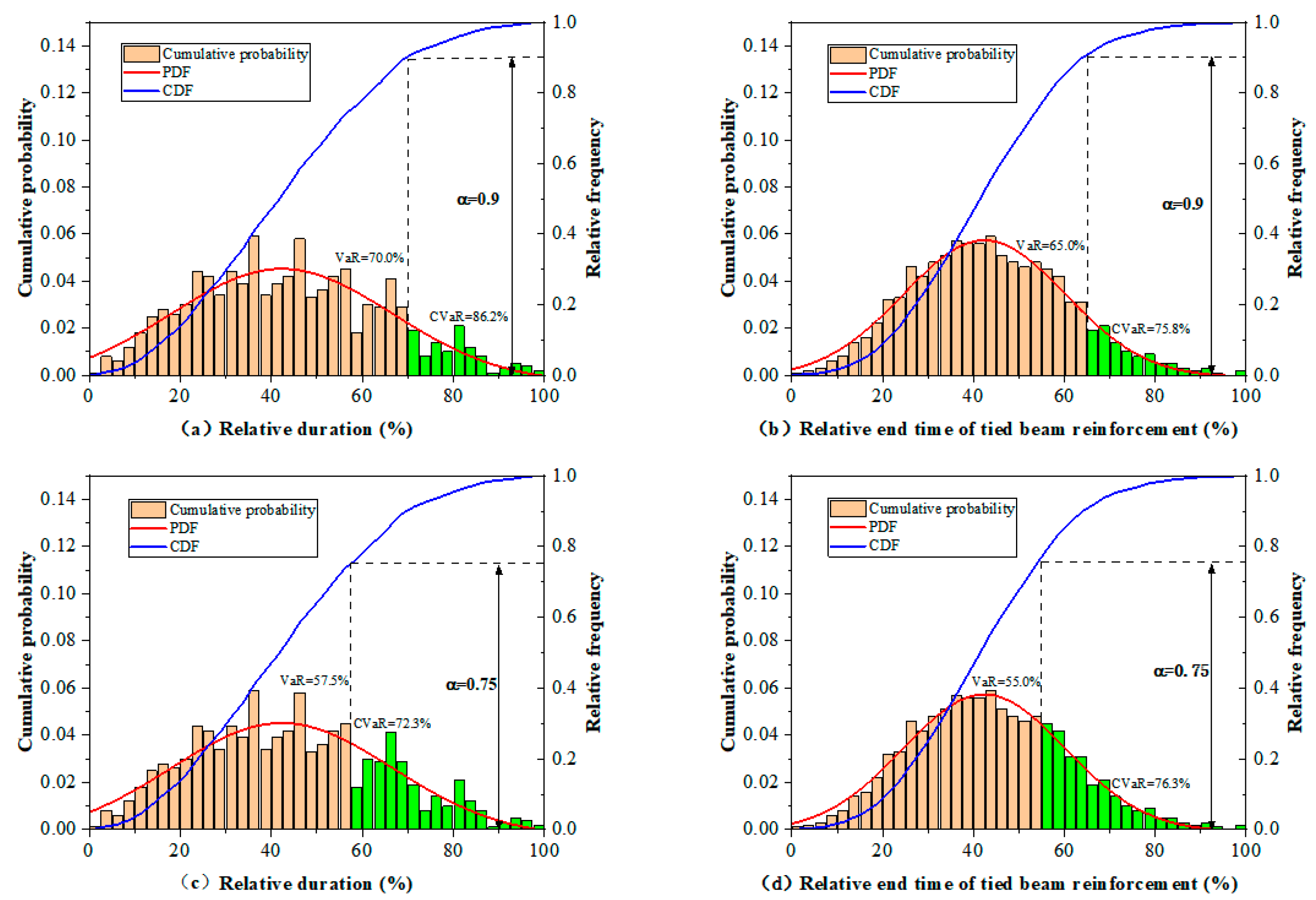
5.2. VaR and CVaR Analysis for Specified Models

5.2.1. VaR and CVaR Analysis of Construction Period

The 50 replicated simulations for each of the 90 labor combinations were fitted to a function image in Figure 9 according to the method described in Section 3.4. The image’s horizontal axis signifies the selected program indicators, the left vertical axis denotes the probability density, and the right vertical axis represents the cumulative distribution. Table 3 offers a comparative analysis of VaR and CVaR for the construction period under various confidence levels. In this research, the relative duration at the confidence level α = 0.9 was firstly chosen for the analysis, and Figure 8a shows the image of the VaR and CVaR function. Under this confidence level, the CDF corresponding to the cumulative distribution of 0.9 was found from the right axis, and the corresponding PDF was obtained, and then the relative duration x under this confidence level was calculated by combining with Equation (4). At the confidence level α = 0.9, we found VaR = 70.0%. Referring to Equation (2), we identified the associated actual duration of 69.69 h. It means that the floor can be completed in 69.69 h at the 90% confidence level. If the floor is not completed in 69.69 h, the expectation of the duration is outside the acceptable range. The new expectation will be 74.56 h, i.e., if 69.69 h is set as the upper limit of the acceptable range, the expected time to complete the floor after exceeding the upper limit will be 74.56 h. Conversely, a project manager who wants to complete the floor in 69.69 h can reverse the above process to arrive at a 90% certainty of completing the floor within that time.
The overestimation of risk incurs additional costs, and the underestimation of risk may lead to irreversible losses [31]. So, an appropriate confidence level needs to be chosen. In order to have a better grasp of the duration, instead of using Alierza’s confidence level of 0.9 for the escalation factor, this paper chooses to use the relative duration with confidence level α = 0.75 (Figure 9c) for comparison because α = 0.75 is more comparable in this case [45]. The floor duration at α = 0.75 was calculated as VaR(0.75) = 65.94 h, CVaR(0.75) = 70.38 h. Combining the durations at the two confidence levels, the degree of certainty was increased by 15% in the case of only a 4 h delay, which is undoubtedly favorable to the grasp of the schedule. Project managers can combine the probability image with fuzzy estimation when grasping the duration, and calculate the corresponding duration prediction after choosing the appropriate confidence level.

5.2.2. VaR and CVaR Analysis of End Time of Tying Beam Reinforcing Bars

Combining a VaR and CVaR analysis can help field managers to extrapolate activity duration. Using tying beam bars as an example, the distribution graph in Figure 9b can be used to find out that VaR(0.9) is 42.54 h and CVaR(0.9) is 45.27h. For α = 0.75 (Figure 9d), VaR(0.75) is 40.01 h and CVaR(0.75) is 45.39 h. Table 4 illustrates a comparison of VaR and CVaR for the completion time of tying beam reinforcing bars at different confidence levels. Research has found that (1) as the confidence level increases, VaR increases and completion time is delayed; (2) as the confidence level increases, CVaR may not necessarily increase, meaning that a conservative completion time may not necessarily be delayed; (3) the amplitude of changes in VaR and CVaR is found to be uncorrelated; and (4) the choice of confidence level is crucial for evaluating the changes in the results, and a low confidence level is not advisable. Thus, in practice, managers need to find the optimal trade-off between reward and risk [24].

5.3. Validation of Results

To test the validity of the findings, the authors interviewed two managers from the case study project and three managers from other projects. The five respondents had an average of 11 years of construction experience. In order to understand how the respondents assessed Takt-time and VaR and CVaR, the authors asked the following questions: (1) Does the step-by-step optimization in Takt-time facilitate the improvement in on-site construction? (2) Is the proposed workforce combination based on the optimization of Takt-time beneficial to the workforce allocation? (3) Does the schedule plan based on the VaR and CVaR analysis facilitate schedule communication?
The interviewees agreed that the step-by-step optimization provided by Takt-time is aligned with the principle of continuous improvement. Through the improvement, the construction plan will be more compacted. At the same time, the workforce combination developed is useful for worker allocation on the site. The VaR and CVaR prediction and analysis graph connected the probability with the corresponding results, so that they have a more solid basis for reporting in the corresponding meetings.

6. Conclusions

This paper applied the Takt-time planning method in a case study project to establish four fast-track simulation models using a three-step optimization and 90 labor combinations to optimize the duration and cost of the project. The optimized result is 20.2% shorter than the actual duration, while the labor cost is reduced by 2.1%.
In construction projects with many repetitive activities, the proposed method can be used to optimize resource utilization based on the project’s unique conditions and preference. In addition, the advantages of the Takt-time scheduling method lie in regulating working time, reducing overtime, and limiting one crew in a certain construction area, which is very beneficial to improve safety and minimize interference of working space.
VaR and CVaR approaches derive a threshold at a given confidence level and provide a way to evaluate and prepare for extreme situations. The VaR approach provides the corresponding probability interchangeable with the actual situation. CVaR provides the optimal scenario for unanticipated situations. This research demonstrated how to implement a VaR and CvaR analysis using outputs from 4500 sets of simulation. The combination of the VaR and CVaR approach can help managers to minimize the chance of blindly choosing the worst combination, and facilitate progress monitoring and effective communication for site management.
The theoretical contributions of this paper are mainly twofold. Firstly, it is the first instance of establishing a research framework that integrates three independent research methods, namely, the Takt-time-based schedule method, Arena’s multi-scenario simulation, and VaR and CvaR’s subjective and objective risk analysis method. This framework can realize a whole set of mechanisms from resource allocation to a scenario change and risk analysis, to achieve resource optimization based on the actual needs of the project and risk control with stability under different scenario changes. This study not only created a new research framework, but also enabled a smooth connection at the data interface level. Secondly, the VaR and CVaR approaches for risk assessment were applied to the field of construction planning. It predicts the results of different construction scenarios based on the managers’ preference and projects’ risk tolerance. In practice, the optimal solution selected among a large number of alternatives and specific application scenarios is useful for project managers to make planning decisions facing uncertainty of job sites and particular priority requirements of projects.
Two future research directions are proposed. First, this paper focused on high-rise residential buildings with a design of standard floors. Future research can be expanded to other types of structures to explore the adaptability of the research framework. Second, the current VAR and CVAR evaluations focus only on the construction schedule, and additional performance indicators such as cost or quality can be added to develop a more comprehensive risk evaluation profile of construction projects.

Author Contributions

Conceptualization, F.D., S.M.H. and M.L.; methodology, F.D. and M.L.; software, F.D. and K.J.; validation, M.L. and Y.Z.; analysis, F.D., M.L. and Y.Z.; writing—original draft preparation, F.D.; writing—review and editing, M.L. and Y.Z.; resources, P.H.; project administration, K.J.; visualization, F.D. and M.L. All authors have read and agreed to the published version of the manuscript.

Funding

This research received no external funding.

Data Availability Statement

The data presented in this study are available on request from the corresponding author. The data are not publicly available due to project restrictions.

Conflicts of Interest

Author Peng Hu was employed by the company New Huayou Construction Engineering Group Co., Ltd. The remaining authors declare that the research was conducted in the absence of any commercial or financial relationships that could be construed as a potential conflict of interest.

Appendix A. Preliminary Organization of Data and Calculations

Buildings 14 00553 i001

Appendix B. Identifying Productivity Distribution Curve for Tying Beam Reinforcing Rebar

Buildings 14 00553 i002

Appendix C. Activity Duration Defined for the Simulation Models (Unit: Hour)

Buildings 14 00553 i003

Appendix D. The Models Generated in Arena Software (an Excerpt)

Buildings 14 00553 i004

Appendix E. Detailed Description of Research Steps

1. Productivity data collection and analysis:
(1)
Collect sufficient productivity data (illustrated in Table 1);
(2)
Calculate productivity (illustrated in Appendix A).
Example: For tying beam reinforcement at B1 on the 14th layer, calculate productivity as follows: A. Divide recorded time data into sessions: “1 person, 6:02–6:47” and “1 person, 8:12–8:34”. B. Calculate tying duration (D) = 67 min. C. Measure beam reinforcement length (P) at B1 = 3.75 m. D. Calculate productivity at B1 as W = D/P = 17.87min/m. E. Apply the same method to determine productivity for other layers and other activities.
2. Identifying productivity distribution curves:
Detailed analysis steps are shown in Appendix B.
3. Takt-Time adjustment:
(1)
Determine working hours based on recorded data.
(2)
Dividing regions for different construction activities.
(3)
Set Takt as 5 or 2.5 h, only allowing one crew in one unit area within the Takt.
(4)
Apply 50% fast-tracking.
4. Model establishment:
Build simulation models and assign variables. Appendix D shows an example.
5. Simulation and data analysis:
Simulate 50 iterations randomly using the productivity function.
Utilize a 95% confidence level for the simulation results.
Record model data into an external table based on the CPM chart (Appendix C).
6. Create a 3D color-mapped plot:
A summary of 90 groups of the labor force for four models is compiled and plotted in Figure 7.
7. Normalize data, and VaR and CvaR analysis:
(1)
Select optimal model data.
(2)
Normalize simulated data from 0 to 1.
(3)
Calculate project parameters using Equation (4).
(4)
Determine VaR and CVaR values based on the selected confidence level using Equations (2) and (3), respectively.

References

  1. Dave, B.; Koskela, L. Collaborative Knowledge Management—A Construction Case Study. Autom. Constr. 2009, 18, 894–902. [Google Scholar] [CrossRef]
  2. Guo, H.; Yu, Y.; Skitmore, M. Visualization Technology-Based Construction Safety Management: A Review. Autom. Constr. 2017, 73, 135–144. [Google Scholar] [CrossRef]
  3. He, C.; Liu, M.; Alves, T.C.L.; Scala, N.M.; Hsiang, S.M. Prioritizing Collaborative Scheduling Practices Based on Their Impact on Project Performance. Constr. Manag. Econ. 2022, 40, 618–637. [Google Scholar] [CrossRef]
  4. Faghihi, V.; Nejat, A.; Reinschmidt, K.F.; Kang, J.H. Automation in Construction Scheduling: A Review of the Literature. Int. J. Adv. Manuf. Technol. 2015, 81, 1845–1856. [Google Scholar] [CrossRef]
  5. Khalesi, H.; Balali, A.; Valipour, A.; Antucheviciene, J.; Migilinskas, D.; Zigmund, V. Application of Hybrid SWARA--BIM in Reducing Reworks of Building Construction Projects from the Perspective of Time. Sustainability 2020, 12, 8927. [Google Scholar] [CrossRef]
  6. Biruk, S.; Rzepecki, Ł. A Simulation Model of Construction Projects Executed in Random Conditions with the Overlapping Construction Works. Sustainability 2021, 13, 5795. [Google Scholar] [CrossRef]
  7. Dasović, B.; Galić, M.; Klanšek, U. Active BIM Approach to Optimize Work Facilities and Tower Crane Locations on Construction Sites with Repetitive Operations. Buildings 2019, 9, 21. [Google Scholar] [CrossRef]
  8. Mohamed, H.H.; Ibrahim, A.H.; Soliman, A.A. Toward Reducing Construction Project Delivery Time under Limited Resources. Sustainability 2021, 13, 11035. [Google Scholar] [CrossRef]
  9. Chen, G.; He, C.; Hsiang, S.; Liu, M.; Li, H. A Mechanism for Smart Contracts to Mediate Production Bottlenecks under Constraints. In Proceedings of the 31st Annual Conference of the International Group for Lean Construction (IGLC), Lille, France, 26 June–2 July 2023; International Group for Lean Construction (IGLC): Lille, France, 2023; pp. 1232–1244. [Google Scholar]
  10. Ballard, G.; Koskela, L.; Howell, G.; Zabelle, T. Production System Design in Construction. In Proceedings of the 9th Annual Conference of the International Group for Lean Construction, Singapore, 6–8 August 2001. [Google Scholar]
  11. Koskela, L.; Ballard, G. What Should We Require from a Production System in Construction? In Proceedings of the Construction Research Congress, Honolulu, HI, USA, 19–21 March 2003; pp. 1–8. [Google Scholar]
  12. Abbasi, S.; Taghizade, K.; Noorzai, E. BIM-Based Combination of Takt Time and Discrete Event Simulation for Implementing Just in Time in Construction Scheduling under Constraints. J. Constr. Eng. Manag. 2020, 146, 04020143. [Google Scholar] [CrossRef]
  13. Lerche, J.; Enevoldsen, P.; Seppänen, O. Application of Takt and Kanban to Modular Wind Turbine Construction. J. Constr. Eng. Manag. 2022, 148, 05021015. [Google Scholar] [CrossRef]
  14. Tommelein, I.D. Work Density Method for Takt Planning of Construction Processes with Nonrepetitive Work. J. Constr. Eng. Manag. 2022, 148, 4022134. [Google Scholar] [CrossRef]
  15. Ibrahim, K.K.; Daniel, C.O. Influence of Project Planning Processes on Construction Project Success in Nigeria. Eur. J. Bus. Manag. 2020, 12, 40–47. [Google Scholar]
  16. Keskiniva, K.; Saari, A.; Junnonen, J.-M. Takt Planning in Apartment Building Renovation Projects. Buildings 2020, 10, 226. [Google Scholar] [CrossRef]
  17. Dlouhy, J.; Binninger, M.; Oprach, S.; Haghsheno, S. Three-Level Method of Takt Planning and Takt Control--A New Approach for Designing Production Systems in Construction. In Proceedings of the 24th Annual Conference of the International Group for Lean Construction, Boston, MA, USA, 20–22 July 2016; pp. 20–22. [Google Scholar]
  18. Akhavian, R.; Behzadan, A.H. Construction Equipment Activity Recognition for Simulation Input Modeling Using Mobile Sensors and Machine Learning Classifiers. Adv. Eng. Inform. 2015, 29, 867–877. [Google Scholar] [CrossRef]
  19. Chen, J.-H.; Yang, L.-R.; Tai, H.-W. Process Reengineering and Improvement for Building Precast Production. Autom. Constr. 2016, 68, 249–258. [Google Scholar] [CrossRef]
  20. Zahraee, S.M.; Esrafilian, R.; Kardan, R.; Shiwakoti, N.; Stasinopoulos, P. Lean Construction Analysis of Concrete Pouring Process Using Value Stream Mapping and Arena Based Simulation Model. Mater. Today Proc. 2021, 42, 1279–1286. [Google Scholar] [CrossRef]
  21. Utku, D.H. The Evaluation and Improvement of the Production Processes of an Automotive Industry Company via Simulation and Optimization. Sustainability 2023, 15, 2331. [Google Scholar] [CrossRef]
  22. Li, P.; Walton, J.R. Evaluating Freeway Service Patrols in Low-Traffic Areas Using Discrete-Event Simulation. J. Transp. Eng. 2013, 139, 1095–1104. [Google Scholar] [CrossRef]
  23. He, C.; Liu, M.; Zhang, Y.; Wang, Z.; Simon, M.H.; Chen, G.; Chen, J. Exploit Social Distancing in Construction Scheduling: Visualize and Optimize Space–Time–Workforce Tradeoff. J. Manag. Eng. 2022, 38, 4022027. [Google Scholar] [CrossRef]
  24. Leite, F.; Cho, Y.; Behzadan, A.H.; Lee, S.; Choe, S.; Fang, Y.; Akhavian, R.; Hwang, S. Visualization, Information Modeling, and Simulation: Grand Challenges in the Construction Industry. J. Comput. Civ. Eng. 2016, 30, 04016035. [Google Scholar] [CrossRef]
  25. Liu, S.; Li, X.; He, C. Study on Dynamic Influence of Passenger Flow on Intelligent Bus Travel Service Model. Transport 2021, 36, 25–37. [Google Scholar] [CrossRef]
  26. Kolny, D.; Kaczmar-Kolny, E.; Dulina, L. Modeling and Simulation of the Furniture Manufacturing and Assembly Process in the Arena Simulation Software. Technol. Autom. Montażu 2023, 119, 13–22. [Google Scholar] [CrossRef]
  27. Göb, R. Estimating Value at Risk and Conditional Value at Risk for Count Variables. Qual. Reliab. Eng. Int. 2011, 27, 659–672. [Google Scholar] [CrossRef]
  28. Hong, L.J.; Hu, Z.; Liu, G. Monte Carlo Methods for Value-at-Risk and Conditional Value-at-Risk: A Review. ACM Trans. Model. Comput. Simul. 2014, 24, 1–37. [Google Scholar] [CrossRef]
  29. Xie, K.; Zhu, S.; Gui, P.; Chen, Y. Coordinating an Emergency Medical Material Supply Chain with CVaR under the Pandemic Considering Corporate Social Responsibility. Comput. Ind. Eng. 2023, 176, 108989. [Google Scholar] [CrossRef]
  30. Bodnar, T.; Lindholm, M.; Niklasson, V.; Thorsén, E. Bayesian Portfolio Selection Using VaR and CVaR. Appl. Math. Comput. 2022, 427, 127120. [Google Scholar] [CrossRef]
  31. Müller, F.M.; Righi, M.B. Comparison of Value at Risk (VaR) Multivariate Forecast Models. Comput. Econ. 2024, 63, 75–110. [Google Scholar] [CrossRef]
  32. Balbás, A.; Balbás, B.; Balbás, R. Differential Equations Connecting VaR and CVaR. J. Comput. Appl. Math. 2017, 326, 247–267. [Google Scholar] [CrossRef]
  33. Avci, M.G.; Avci, M. An Empirical Analysis of the Cardinality Constrained Expectile-Based VaR Portfolio Optimization Problem. Expert Syst. Appl. 2021, 186, 115724. [Google Scholar] [CrossRef]
  34. Fan, W.; Tan, Z.; Li, F.; Zhang, A.; Ju, L.; Wang, Y.; De, G.; Lund, H.; Kaiser, M.J. A Two-Stage Optimal Scheduling Model of Integrated Energy System Based on CVaR Theory Implementing Integrated Demand Response. Energy 2023, 263, 125783. [Google Scholar] [CrossRef]
  35. Oulidi, A.; Charpentier, A. Estimating Allocations for Value-at-Risk Portfolio Optimzation. Available online: https://ssrn.com/abstract=1023911 (accessed on 3 February 2024).
  36. Altun, E.; Tatlıdil, H.; Özel, G. Conditional ASGT-GARCH Approach to Value-at-Risk. Iran. J. Sci. Technol. Trans. A Sci. 2019, 43, 239–247. [Google Scholar] [CrossRef]
  37. Balbás, A.; Balbás, B.; Balbás, R. VaR as the CVaR Sensitivity: Applications in Risk Optimization. J. Comput. Appl. Math. 2017, 309, 175–185. [Google Scholar] [CrossRef]
  38. Zheng, H. Efficient Frontier of Utility and CVaR. Math. Methods Oper. Res. 2009, 70, 129–148. [Google Scholar] [CrossRef]
  39. Hu, Z.; Wei, C.; Yao, L.; Li, L.; Li, C. A Multi-Objective Optimization Model with Conditional Value-at-Risk Constraints for Water Allocation Equality. J. Hydrol. 2016, 330–342. [Google Scholar] [CrossRef]
  40. Chen, G.; Liu, M.; Zhang, Y.; Wang, Z.; Hsiang, S.M.; He, C. Using Images to Detect, Plan, Analyze, and Coordinate a Smart Contract in Construction. J. Manag. Eng. 2023, 39, 04023002. [Google Scholar] [CrossRef]
  41. Javanmardi, A.; He, C.; Hsiang, S.M.; Abbasian-Hosseini, S.A.; Liu, M. Enhancing Construction Project Workflow Reliability through Observe–Plan–Do–Check–React Cycle: A Bridge Project Case Study. Buildings 2023, 13, 2379. [Google Scholar] [CrossRef]
  42. Tang, L.; Ling, A. A Closed-Form Solution for Robust Portfolio Selection with Worst-Case CVaR Risk Measure. Math. Probl. Eng. 2014, 2014, 494575. [Google Scholar] [CrossRef]
  43. Schniederjans, M.J.; Schniederjans, D.; Cao, Q. Value Analysis Planning with Goal Programming. Ann. Oper. Res. 2017, 251, 367–382. [Google Scholar] [CrossRef]
  44. Caron, F.; Fumagalli, M.; Rigamonti, A. Engineering and Contracting Projects: A Value at Risk Based Approach to Portfolio Balancing. Int. J. Proj. Manag. 2007, 25, 569–578. [Google Scholar] [CrossRef]
  45. Joukar, A.; Nahmens, I. Estimation of the Escalation Factor in Construction Projects Using Value at Risk. In Proceedings of the Construction Research Congress 2016, San Juan, Puerto Rico, 31 May–2 June 2016. [Google Scholar]
  46. Elena Bruni, M.; Beraldi, P.; Guerriero, F.; Pinto, E. A Scheduling Methodology for Dealing with Uncertainty in Construction Projects. Eng. Comput. 2011, 28, 1064–1078. [Google Scholar] [CrossRef]
  47. Rahimi, M.; Ghezavati, V. Sustainable Multi-Period Reverse Logistics Network Design and Planning under Uncertainty Utilizing Conditional Value at Risk (CVaR) for Recycling Construction and Demolition Waste. J. Clean. Prod. 2018, 172, 1567–1581. [Google Scholar] [CrossRef]
  48. He, C.; Liu, M.; Zhang, Y.; Wang, Z.; Hsiang, S.M.; Chen, G.; Li, W.; Dai, G. Space–Time–Workforce Visualization and Conditional Capacity Synthesis in Uncertainty. J. Manag. Eng. 2023, 39, 04022071. [Google Scholar] [CrossRef]
  49. Filippi, C.; Guastaroba, G.; Speranza, M.G. Conditional Value-at-Risk beyond Finance: A Survey. Int. Trans. Oper. Res. 2020, 27, 1277–1319. [Google Scholar] [CrossRef]
  50. Charpentier, A.; Oulidi, A. Estimating Allocations for Value-at-Risk Portfolio Optimization. Math. Methods Oper. Res. 2009, 69, 395–410. [Google Scholar] [CrossRef]
  51. De Schepper, A.; Heijnen, B. How to Estimate the Value at Risk under Incomplete Information. J. Comput. Appl. Math. 2010, 233, 2213–2226. [Google Scholar] [CrossRef]
  52. Heinkenschloss, M.; Kramer, B.; Takhtaganov, T.; Willcox, K. Conditional-Value-at-Risk Estimation via Reduced-Order Models. SIAM/ASA J. Uncertain. Quantif. 2018, 6, 1395–1423. [Google Scholar] [CrossRef]
  53. Almeida, J.; Soares, J.; Lezama, F.; Vale, Z. Robust Energy Resource Management Incorporating Risk Analysis Using Conditional Value-at-Risk. IEEE Access 2022, 10, 16063–16077. [Google Scholar] [CrossRef]
  54. AbouRizk, S. Role of Simulation in Construction Engineering and Management. J. Constr. Eng. Manag. 2010, 136, 1140–1153. [Google Scholar] [CrossRef]
  55. Romanko, O.; Mausser, H. Robust Scenario-Based Value-at-Risk Optimization. Ann. Oper. Res. 2016, 237, 203–218. [Google Scholar] [CrossRef]
  56. Lehtovaara, J.; Seppänen, O.; Peltokorpi, A.; Kujansuu, P.; Grönvall, M. How Takt Production Contributes to Construction Production Flow: A Theoretical Model. Constr. Manag. Econ. 2021, 39, 73–95. [Google Scholar] [CrossRef]
Figure 1. Research flowchart.
Buildings 14 00553 g001
Figure 2. CPM diagram: orange arrows are critical paths.
Buildings 14 00553 g002
Figure 3. Arena Simulation model logic diagram.
Buildings 14 00553 g003
Figure 4. Floor plan.
Buildings 14 00553 g004
Figure 5. Part of the construction activity real photos.
Buildings 14 00553 g005
Figure 6. Construction work areas.
Buildings 14 00553 g006
Figure 7. Duration for different labor combinations: (a) no-fast-track Takt = 5; (b) no-fast-track Takt = 2.5; (c) 50%-fast-track Takt = 2.5; (d) H-B area delineated and 50%-fast-track Takt = 2.5.
Buildings 14 00553 g007
Figure 8. Cost for different labor combinations: (a) no-fast-track Takt = 5; (b) no-fast-track Takt = 2.5; (c) 50%-fast-track Takt = 2.5; (d) H-B area delineated and 50%-fast-track Takt = 2.5.
Buildings 14 00553 g008
Figure 9. Sample calculations of VaR and CVaR: (a) relative duration for α = 0.9; (b) relative end time of tying beam reinforcing bars for α = 0.9; (c) relative duration for α = 0.75; (d) relative end time of tying beam reinforcing bars for α = 0.75.
Buildings 14 00553 g009
Table 1. Sample data collection.
Date30 July 2022Floor15th Floor
Job categoryBar placersNumber of workers1 person
Working positionDataStarting time16:40
ActivityTying of wall and column reinforcementEnd time17:05
Description of activitiesSet column hoops, tied lap vertical structural bars
Table 2. Comparison of duration under 4 models (in hours).
No-Fast-tr.
Takt = 5
No-Fast-tr.
Takt = 2.5
Fast-tr.
Takt = 2.5
Subarea-Fast-tr.
Takt = 2.5
Minimum69.367.1857.9555.28
Maximum87.2684.974.5370.81
Average77.9875.5565.7362.55
Average/No-fast-tr.
Takt = 5
10.9690.8430.802
Average/No-fast-tr.
Takt = 2.5
/10.870.828
Average/Fast-tr.
Takt = 2.5
//10.952
Table 3. VaR and CVaR comparison of the construction period.
Confidence Level αα = 90%α = 75%Results of
α = 90% vs. α = 75%
VaRrelative value70.0%57.5%reduced by 12.5%
actual value69.69 h65.94 hreduced by 3.75 h
CVaRrelative value86.2%72.3%reduced by 13.9%
actual value74.56 h70.38 hreduced by 4.18 h
Results of
VAR vs. CVAR
relative value increased by 16.2%
actual value increased by 4.87 h
relative value increased by 14.8%
actual value increased by 4.44 h
Table 4. VaR and CVaR comparison of end time for tying beam bars.
Confidence Level αα = 90%α = 75%Results of
α = 90% vs. α = 75%
VaRrelative value65.0%55.0%reduced by 10.0%
actual value42.54 h40.01 hreduced by 2.53 h
CVaRrelative value75.8%76.3%increased by 0.5%
actual value45.27 h45.39 hincreased by 0.12 h
Results of
VAR vs. CVAR
relative value increased by 10.8%
actual value increased by 2.73 h
relative value increased by 21.3%
actual value increased by 5.38 h
Disclaimer/Publisher’s Note: The statements, opinions and data contained in all publications are solely those of the individual author(s) and contributor(s) and not of MDPI and/or the editor(s). MDPI and/or the editor(s) disclaim responsibility for any injury to people or property resulting from any ideas, methods, instructions or products referred to in the content.

