Comparison of Linear and Nonlinear Procedures for the Analysis of the Seismic Performance of Straight Multi-Span RC Bridges

Abstract

The assessment of the seismic performance of transportation infrastructures is of primary importance for the management of the aftermath of an earthquake. To perform such an assessment, various modeling approaches characterized by different levels of accuracy are available and modern seismic design codes provide recommendations about their use. Non-linear time-history analysis (NLTHA) is acknowledged as the most reliable method, but is difficult to implement and is computationally expensive. This paper aims to investigate the viability of less complex methods, but with low computational cost, for the assessment of straight, multi-span bridges and compare their performance against the results of NLTHA in order to quantify the expected accuracy. The study is developed considering three bridge archetypes with either simply-supported or continuous-deck layouts, representative of typical features of the Italian bridge stock. The bridges are analyzed first through nonlinear dynamic analyses, to define the benchmark solution; then linear dynamic analyses, such as Linear Time-History and Response Spectrum Analysis, nonlinear static analyses, such as MPA (Modal Pushover Analysis), and Equivalent Static Analysis are considered. A comparison among the examined procedures is eventually proposed, highlighting the strengths and weaknesses of each approach.

1. Introduction

Bridges are a key component of the transportation infrastructure system. Given their importance for the economic and social development of communities, the design and construction of bridges should ensure their sustainability throughout their lifetime. However, in developed countries, e.g., Italy [1], most existing bridges were designed according to outdated codes that did not address current requirements, including seismic resistance. In this regard, it is necessary to emphasize that bridges perform a strategic function in civil protection plans for emergency management and must remain functional in the aftermath of an extreme event. Therefore, the assessment of their potential performance in the case of ground motions is of paramount importance in earthquake-prone countries.

The seismic demand of a bridge can be assessed through an analysis performed on a mathematical model that describes the behavior of the superstructure and substructure and the characteristics of the ground motion. To perform this analysis, modern seismic design codes [2,3,4] recommend different approaches, characterized by different levels of accuracy in relation to the assumed structural model. To provide a reliable estimate of the seismic response of the structure, the model should include the actual geometry, boundary conditions, gravity load, mass distribution, energy dissipation, and nonlinear properties of all the main components of the bridge. On the other hand, increasing the complexity of the mathematical model involves longer times for modeling and analysis, a demand for greater computing capabilities, and, finally, the designer’s ability to handle more complex models.

Modeling and analysis procedures can be divided into linear and nonlinear approaches. In linear models, the important properties are the elastic stiffnesses of the structural members, which are usually simple and well-standardized. In nonlinear analyses, two categories of nonlinearities must be addressed in the model. The first category includes the nonlinear stress–strain relationships of materials (the required properties include yield strength, post-yield behavior, and stiffnesses degradation under cyclic loading, in addition to the initial elastic stiffness), as well as the presence of gaps, dampers, or nonlinear springs in special bridge components. The second category consists of geometric nonlinearities that account for P-Δ effects (second order effects) and large deformation situations, where the equilibrium condition is determined by the deformed shape of the structure. This second type of nonlinearity is incorporated directly into the analysis algorithm. However, the precise definition of the material and geometric nonlinearities in the model is a delicate task that requires expert judgment and a deep understanding of structural behavior, as the analysis results are generally sensitive to even small variations in input parameters. When an elastic model is used, the analysis can reproduce the actual structural response only if the stresses in the structural members do not exceed the elastic limit of their materials. Above this level of demand, the forces and displacements calculated using a linear analysis differ considerably from the forces and displacements actually triggered in the structure. A linear model fails to represent many sources of the inelastic bridge response, including the cyclic yielding of structural components, the opening and closing of deck expansion joints, the engagement, yielding and release of constraints, and the complex nonlinear behavior of abutments and foundations. In linear analyses, the forces in the structural members are computed, and the performance is assessed using strength demand/capacity (D/C) ratios.

Nonlinear analyses provide more reliable predictions of internal forces and deformations in the bridge members and can be used for the design of the bridge subsystems or the evaluation of the bridge’s global capacity and ductility. In nonlinear analysis, inelastic deformations as also calculated, and the performance is assessed using both deformation and strength D/C ratios.

In recent years, studies have been undertaken to develop accurate and practical analysis procedures to assess the seismic performance of existing bridges. Nonlinear time-history analysis (NLTHA) is acknowledged, by far, to be the most reliable method to assess the seismic response of structures. However, it requires the formulation of complex mathematical models of the real structure, the analyses are time-consuming and in addition, the accuracy of the results depends on the assumptions made on the seismic action. To reduce the computational burden, research has investigated alternative procedures, mainly related to multi-span continuous-deck bridges, using nonlinear static analysis [5,6,7,8,9,10,11,12,13,14,15]; the debate to validate such procedures is still ongoing. Paraskeva et al. adapted modal pushover analysis to bridges, developing a multimodal pushover analysis procedure that was applied to two case study bridges, consisting of a 12-span RC (reinforced concrete) structure with a prestressed concrete box girder and characterized by a large curvature in plan, and of a 3-span RC overpass with the deck monolithically connected to the piers [12,16]. Araújo et al. studied the applicability of pushover analyses to archetypes of irregular-in-plan curved bridges and compared the results to those provided by NLTHA [17]. Kohrangi et al. investigated the reliability of four nonlinear static analyses (N2, Modal push over, Adaptive capacity spectrum method and Extended N2 method) for evaluating the seismic performance of RC bridges characterized by different levels of irregularities [18]. Nuti and co-workers developed a method for interpreting modal pushover analyses (IMPA) [19,20], presenting an application to bridges subjected to near-fault ground motions [21]. The application of multi-modal pushover analyses to six bridge typologies representative of the Italian Highway Network was investigated by Crespi [22]; the typologies included examples of both simply supported and continuous superstructures.

The level of accuracy required for the analysis may depend on whether its scope is to provide a refined structure-specific risk assessment or to provide portfolio-scale risk predictions aiming at identifying high-risk structures that will be subjected to further in-depth analysis. To this scope, simplified procedures involving a lower computational demand for analysts in comparison to advanced nonlinear methodologies, appear a viable alternative for analyzing several structures in a short time, representing a viable solution for portfolio-scale risk-informed prioritization [23]. Simplified strategies for simply-supported bridges based on the individual pier model [24], also endorsed in the Italian Building Code NTC 2018 [2], are described in the cited reference [23]. For hyperstatic, continuous-deck bridges, a satisfactory trade-off between the simplicity of the analysis and the accuracy of the results can be achieved using the Displacement-Based Assessment (DBA) method [25,26,27,28], which was further extended to include the effects of higher modes [29,30,31,32] and soil-structure interaction [33]. An alternative displacement-based pseudo-pushover method was proposed by Gentile et al. for RC hyperstatic bridges [34], and further improved by Nettis et al. [35] for bridges governed by higher modes.

In this context, the aim of this study, which is mainly addressed to practitioners involved in the seismic assessment of bridges, is to present a review and evaluation of some of the seismic analysis procedures recommended in the codes, starting from simplified static/dynamic linear approaches to nonlinear static methods and well-known nonlinear time history analysis. In particular, reference has been made to the Italian Building Code (IBC) [2] and the Eurocode 8 [3,4]. Popular linear and nonlinear techniques have been selected among those prescribed in the cited codes, and three archetypes of multi-span RC ordinary bridges with either simply supported or continuous deck, which represent the most common bridge typologies in Europe, have been analyzed. A comparison between the different techniques has been eventually proposed, highlighting the strengths and weaknesses of each approach.

The study will consider examples of multi-span bridges with straight decks. The analysis of curved multi-span bridges is complicated by the torsional forces induced by the curvature and requires dedicated approximate methods that account for the curvature. This is out of the scope of the present work.

2. Examined Procedures

Five linear and nonlinear procedures recommended in the codes [2,3,4] have been considered in the study. They are the Equivalent Static Analysis (ESA), the Modal Pushover Analysis (MPA), the Response Spectrum Analysis (RSA), the Linear Time History Analyses (THA), and the Nonlinear Time History Analysis.

2.1. Equivalent Static Analysis

Equivalent Static Analysis is a simplified method typically used to estimate displacement demands and to perform preliminary evaluations of ordinary structures. The Italian Building Code [2] and the Eurocode [4] provide a list of conditions for the applicability of this technique to bridges. ESA is allowed in the case of structures or individual frames with well-balanced spans and uniformly distributed stiffness where the response can be captured by a predominant translational mode of vibration. According to the Eurocode [4], ESA can be performed in the longitudinal direction of continuous-deck bridges, when the mass of the piles carrying the seismic forces is less than 20% of the total mass of the superstructure, and in the transverse direction when the structural system is approximately symmetric about the center of the deck (i.e., maximum eccentricity less than 5% of the deck length). In the case of simply-supported bridges, ESA is allowed when no significant interaction occurs between the piles, and the mass of the piles carrying the seismic forces is less than 20% of the total mass of the superstructure.

The seismic demand is represented by an equivalent static horizontal force defined as the product of the tributary mass times the spectral acceleration from the 5% damped Acceleration Spectrum [36]. In the case of bridges, the spectral acceleration is determined by the natural period of the pile-superstructure system, and the equivalent horizontal static force is applied at the height of the center of mass of the superstructure and distributed horizontally in proportion to the actual mass distribution. The internal forces, reactions and displacements of the purely elastic system are hence provided from the analysis.

In order to account for the nonlinear resources of the structure, the codes [2,3] recommend estimating the approximated nonlinear strength demand by reducing the full elastic seismic demand by means of the behavior factor (also called q factor in [2]) depending on the energy dissipation capacity of the structural system.

2.2. Modal Pushover Analysis

The Modal Pushover Analysis, initially developed by Chopra and Goel [37,38] to assess the seismic response of unsymmetrical-in-plan buildings, is an extension of the static pushover analysis that has become a popular performance-based design tool for existing and new structures. The purpose of the pushover analysis is to estimate the expected performance of a system by evaluating its strength and deformation demands by means of static nonlinear analysis and comparing these demands to available capacities at the target performance levels. The method relies on the assumption that the response of the structure is controlled by its fundamental mode, and the structure is subjected to monotonically increasing lateral forces with an invariant spatial distribution until a predetermined target displacement is reached at the monitoring point. Modal Pushover Analysis (MPA) is an extension of the static pushover analysis to consider higher mode effects, under the assumption that the uncoupling of modal responses is still valid in the inelastic stage. The seismic response of each mode is determined by pushing the structure to its modal target displacement with an invariant modal lateral force distribution; the global response is obtained by combining the responses of each mode according to a certain rule (e.g., SRSS, CQC). Since the higher modes are taken into consideration, MPA fits the real structural behavior better than conventional pushover analysis [37], especially in the case of bridges, where higher modes play a more critical role than in buildings. However, in MPA the lateral load patterns are generally assumed to remain constant after yielding, an approximation similar to the one made in standard pushover analysis. Although the superposition of modal responses does not apply in the inelastic range, where modes are not uncoupled, Chopra and Goel have shown that the associated error is typically smaller than in the case where superposition is carried out at the level of loading [38]. Some applications of MPA to bridges can be found in the cited references [12,16].

2.3. Response Spectrum Analysis

The Response Spectrum Analysis is an elastic procedure that generally results in reasonable estimates of displacements and internal forces in structural systems that remain essentially elastic under load.

For each considered natural mode, a static analysis is performed for the entire structure under a set of equivalent forces. The resulting modal static response is then multiplied by the spectral acceleration to obtain the peak modal response. Such a procedure reduces the dynamic analysis to a series of static analyses, thus avoiding the lengthy computation required from NLTHA [36]. It is possible to account for nonlinear effects and plastic resources of the structure by reducing the full elastic seismic demand by means of the behavior factor [2,3,4]. Though the distribution of forces resulting from linear analyses may have little similarity to that expected during the actual earthquake, the concept of using a factor in design to reduce forces has been adopted by most seismic codes, e.g., [2,3,4], in order to account for the nonlinear response of the structure associated with the material, the structural system and the design procedures.

RSA is considered a dynamic analysis technique since it makes use of the vibration properties of the structure, including the natural periods, modes, and modal damping ratios, as well as the dynamic characteristics of the ground motions considered. All modes which provide a significant contribution to the total structural response must be taken into account. According to the Eurocode [4], this condition is deemed as satisfied when the sum of the effective modal masses for the modes considered in the analysis, (ΣM_i)_c, represents at least 90% of the total mass M of the bridge. Alternatively, if the sum of the effective modal masses is at least 70% of the total mass of the bridge, RSA can be used, providing that the seismic action effects calculated by the analysis are multiplied by (ΣM_i)_c [4].

RSA can be used for linear dynamic analysis of structures, but not for nonlinear. The main reason is that response spectrum analysis depends on superposition, which does not apply to nonlinear behavior. Therefore, in the case of standard bridges with significant nonlinear behavior and nonstandard or important bridges, it is necessary to use step-by-step integration, also known as time history or response history analysis. Nevertheless, RSA is generally considered enough accurate for structural design, and it represents one of the most popular analysis methods among practitioners.

A major limitation of RSA is related to the combination of effects. Because of the statistical method used to combine the results, response spectra results can be confusing or misleading to engineers who are not familiar with the process. The confusion is usually associated with the fact that any single response spectra result is correct, but it is not known whether the sign of that result should be positive or negative. This results in a number of limitations that should be considered when using response spectra analysis. Therefore, the selected modal combination rule may lead to significant inaccuracy when computing the modal contribution to the total response [36]. The classical approach is to use the absolute sum of the maximum response quantities obtained for each mode. The assumption behind this is that in all modes the peak response quantities occur at the same time instant, which leads to very conservative design parameters. The alternative common approach is to use the Square Root of the Sum of the Squares, SRSS, of the peak response quantities in each mode of vibration. This approach assumes that the peak modal response quantities are statistically independent. For three-dimensional structural systems in which a large number of periods of vibration are close, this assumption is not justified [39]. The third approach is to use the Complete Quadratic Combination, CQC, to add the peak modal response quantities [40]. The key characteristic of the CQC method is the ability to distinguish the relative signs of peak modal responses and, therefore, eliminate some of the errors that will be observed by using absolute sum and SRSS methods.

2.4. Nonlinear Time History Analysis

Nonlinear Time History Analysis (NLTHA) is a rigorous numerical method consisting of the direct numerical integration of the differential equations of motion by considering the inelastic deformation of the structural members. The loading is formulated in terms of foundation displacement or ground motion acceleration, and the structural forces and displacements are directly determined through dynamic analysis using suites of ground motion records. The dynamic responses in terms of displacement, velocity, and acceleration can be determined by the time-history analysis; thus, the structural internal forces and deformations are obtained at each time step over the total duration of the accelerogram [2].

Each bridge possesses predominating mode shapes and frequencies, which are excited according to the frequency content of the ground motion. The calculated bridge response is highly sensitive to the characteristics of individual ground motions [36]. Therefore, a time-history analysis should be performed using different earthquake histories to ensure that all the significant modes are excited. The use of artificial accelerograms was attractive in the past years since it allowed for the generation of spectrum-compatible compatible time-series in those cases where natural accelerograms were not available [41]. Today, thanks to the growing availability of strong motion databases, the use of ground motion time histories recorded during real earthquakes is preferred [42]. The selection, scaling and application of ground motions to the structural model must be, therefore, carried out according to code recommendations. Since seismic motions can excite the higher frequencies of the structure, neglecting the higher modes of the system may result in significant errors. The number of degrees of freedom and the modes considered in the analysis capture at least 90% of the structural mass in both the longitudinal and transverse directions [3].

The main disadvantage of NLTHA lies in the high computational and analytical efforts required and the large amount of output information provided [36]. Despite these challenges, the evaluation of the bridge capacity by NLTHA yields accurate results, since it accounts for the redistribution of internal forces occurring in the inelastic range within the structure. Therefore, NLTHA allows for the design of each member, and therefore, is not designed for maximum peak values, e.g., by the response spectrum method, but for the actual forces produced in the structure during dynamic excitation.

The numerical stability and accuracy of NLTHA are affected by the methods employed for solving the equations of motion of the structure. The most general approach is the direct numerical integration of the dynamic equilibrium equations at a discrete point in time. This analysis is started at the undisturbed static condition of the structure and repeated throughout the duration of the ground motion input in equal time increments to obtain the complete history of the structural response under a specified excitation.

Direct explicit integration methods are very fast, as they do not require iteration at each time step [36,41]. They allow for any kind of damping and nonlinearity in the model; however, they require very small time intervals to obtain stable results and consequently yield large and unnecessary amounts of output data. On the other hand, direct implicit integration schemes of differential equations of motion require iteration at each time step to achieve equilibrium and involve huge calculations to solve large sparse matrices [43]. They also allow for any kind of damping and nonlinearity in the structural model and tolerate longer time intervals due to the unconditional stability of the results using certain parameters. Implicit integration methods include the Newmark family, the Hilber–Hughes–Taylor and the Chung and Hulbert Method [44,45,46].

2.5. Linear Time History Analysis

For the design of regular structures where the inelastic behavior is predictable, and/or in case of moderate or weak seismicity, where low engagement of inelastic resources is expected, NLTHA may be unnecessary and computationally expensive. For such structures, Linear Time History Analysis (LTHA) can provide sufficient accuracy with limited computational effort. In LTHA, a step-by-step analysis of the dynamic response of the structure is performed like in NLTHA, but all sources of nonlinearity, both geometrical and related to materials’ inelastic behavior, are disregarded. As stated in the Commentary to IBC [47], LTHA is not prescribed in the Italian Building Code; however, it is allowed in the Eurocode Part 2 [4] §4.2.3.1. In this regard, it must be mentioned that the Eurocode recommends using a set of accelerograms compatible with the elastic spectrum for LTHA, as prescribed also for NLTHA, without accounting for the behavior factor ([4], §3.2.3.1.1).

Though the analysis is less accurate than for NLTHA, LTHA features some advantages over static methods, such as the ability to account for multidirectional ground motions (for static methods design guidelines recommend some combination rules, e.g., 100% of the reactions obtained in one direction and 30% in the other), and the availability of time histories of the response quantities. The knowledge of the time histories of internal forces, deformations and accelerations will give an understanding of the dynamic behavior of the bridge which cannot be provided by static methods. In fact, regardless of the method used to superimpose the results, the modal response spectrum analysis will produce positive maximum response quantities that are not a function of time. Consequently, a plot of the deformed shape of the structure under RSA has little meaning and cannot reliably be used to assess nonstructural damage. Further, in the design of structural elements under combined axial load and bending, in static methods, the maximum force quantities are considered, assuming that the maximum axial load and bending moments will occur at the same time, leading to a conservative design.

For solving the equations of motion of the structure, a modal solution is a viable methodology for linear elastic systems, and it results in some cases in reduced computational effort together with reliable results [36].

3. Case Studies

Three archetype RC bridges are considered in the study: two of them are simply supported bridges and the third is a bridge with a continuous deck. The first bridge has frame piles, each composed of three circular columns and a pile cap, and the deck consists of a concrete slab supported from T-shaped beams. The second bridge has circular piles; the spans are 35 m long with V-shaped beams. The third bridge has rectangular hollow section piles and a 35 m span box-girder deck. The selected typologies are the most common in the Italian stock, where they represent more than 90% of existing bridges [1,5], and the dimensions of the decks correspond to typical values in Italian practice [48]. The piles were designed in order to account in the study for different behaviors. The frame piles in the first bridge have different capacities in the two horizontal directions, with low resources in the longitudinal direction. The circular piles in the second bridge have the same strength and stiffness in both longitudinal and transverse bridge directions. Eventually, the rectangular hollow section of the piles of the third bridge is characterized by a very high sectional capacity and is commonly used for tall piles. The dimensions and reinforcement of the piles were taken from the literature, as they will be defined later in the paper.

Three seismic scenarios relevant to as many seismic zones according to the Italian Building Code [2] are examined, corresponding to the municipalities of Reggio Calabria for zone 1 (high seismicity zone with PGA > 0.25 g), Sirmione for zone 2 (medium-high seismicity zone with 0.15 g < PGA ≤ 0.25 g) and Pavia for zone 3 (medium-low seismicity zone, with 0.05 g < PGA ≤ 0.15 g).

3.1. Bridge Characteristics

The three case studies are 4-span reinforced concrete (RC) bridges with different geometries of both superstructures and substructures. For all bridges, the same material properties are assumed: concrete for piles is C25/30, with Young’s modulus E_c = 31,476 MPa and characteristic cylindrical strength f_ck = 25 MPa; steel for the rebar is FeB44k, with Young’s modulus E_s = 200 GPa, characteristic yield strength f_yk = 430 MPa and characteristic tensile strength at break f_tk = 540 MPa.

3.1.1. Bridge 1

The bridge has a simply supported deck with four isostatic spans of 20 m each and is supported from three frame piles with the same height of 5 m according to the layout sketched in Figure 1.

Each pile consists of three circular columns with a 1 m diameter connected at the top by a pile cap (Figure 2a). Each column is reinforced with 12φ18 longitudinal bars arranged circumferentially. The transverse reinforcement consists of φ10 stirrups with 20 cm spacing. The longitudinal and the transverse reinforcement ratios are ρ_s = 0.4% and ρ_w = 0.09% [49,50], respectively.

The deck has a concrete slab and four T-shaped beams of 20 m length (Figure 2b). The relevant characteristics in terms of geometry and loads are summarized in

Table 1. Deck characteristics for Bridge 1.

Property	Value	Unit
A	5.434	m2
γcls	25	kN/m3
g1	135.85	kN/m
g2	47	kN/m
L	20	m
GSpan	3657	kN
Q	276	kN

A = area; γ_cls = weight for unit volume; g₁ = permanent structural load; g₂ = permanent non-structural load; L = span length; G_Span = Span weight; Q = variable load.

.

The bearing layout of each isostatic span consists, in the longitudinal bridge direction, of a fixed axis and a movable axis, while in the transverse direction, the rigid body movement of the deck is prevented (Figure 3); rotations are permitted about the transverse axis. In terms of seismic mass distribution, in the longitudinal direction, the seismic mass acting on each pile is the mass of the rigidly connected span; in the transverse direction, the seismic mass acting on a pile is still equal to the mass of a span as each pile supports half of the seismic mass of the two isostatic spans transversely connected to the pile.

3.1.2. Bridge 2

The bridge has a simply supported deck with four isostatic spans of 35 m each, and is supported by three piles with circular cross-sections and different heights, simulating the situation of a bridge crossing a small valley; the two external piles are 5 m high, while the central pile is 10 m high (Figure 4). The bearing layout is the same as for Bridge 1 (Figure 3), providing the same distribution of seismic masses on the piles.

The piles have a single shaft with a circular cross-section of 2 m diameter (Figure 5). The pile shafts have a longitudinal reinforcement consisting of 24φ26 bars for the 5 m-high pile and 32φ30 bars for the 10 m-high pile. The transverse reinforcement of all piles consists of φ16 stirrups with 15 cm spacing (adapted from [49,50]).

The deck has three V-shaped beams supporting the concrete slab (Figure 6). The relevant characteristics in terms of geometry and loads are summarized in

Table 2. Deck characteristics for Bridge 2.

Property	Value	Unit
A	6.732	m2
γcls	25	kN/m3
g1	168.3	kN/m
g2	47	kN/m
L	35	m
GSpan	7535.5	kN
Q	438	kN

A = area; γ_cls = weight for unit volume; g₁ = permanent structural load; g₂ = permanent non-structural load; L = span length; G_Span = span weight; Q = variable load.

.

3.1.3. Bridge 3

The bridge has a continuous deck with four spans of 35 m each, supported by three piles with the same height of 10 m, according to the layout sketched in Figure 7.

The piles have a rectangular hollow section with dimensions of 200 × 550 cm (Figure 8). The longitudinal reinforcement consists of 70φ24 steel bars, and the transverse reinforcement is composed of stirrups with four arms and a diameter of φ14, spaced at 15 cm [49,50].

The superstructure is a continuous box girder. The cross-section is shown in Figure 9, and the relevant characteristics in terms of geometry and loads are given in

Table 3. Deck characteristics for Bridge 3.

Property	Value	Unit
A	12.54	m2
γcls	25	kN/m3
g1	313.5	kN/m
g2	47	kN/m
Ltotal	140	m
GDeck	50,470	kN
Q	1402	kN

A = area; γ_cls = weight for unit volume; g₁ = permanent structural load; g₂ = permanent non-structural load; L_total = deck length; G_Deck = deck weight; Q = variable load.

.

The bearing layout of Bridge 3 is shown in Figure 10. In the longitudinal direction, there is a fixed axis in the center of the deck, corresponding to the central pile, and four movable axles corresponding to the two external piles and the abutments. The multidirectional bearings on the two abutments and on the external piles are provided with seismic shear keys that are engaged in an earthquake. Therefore, when the bridge is hit by the ground motion all the axes become fixed and the seismic action is resisted by all the superstructures, which behave as an in-parallel system. This solution is aimed at avoiding overloading a single pile as it would occur in the case of a single fixed axis.

Table 4. Moment at first yielding of piles of the case study bridges.

Bridge	Pile	MRd,y [kNm]	MRd,x [kNm]
Bridge 1	P1, P2, P3	2959	7860
Bridge 2	P1, P3	9280	9280
	P2	13,258	13,258
Bridge 3	P1, P2, P3	19,915	51,633

M_Rd,y = moment at yielding of the pile in the longitudinal bridge direction; M_Rd,x = moment at yielding of the pile in the transverse bridge direction. P1 and P3: external piles; P2: central pile (Figure 1, Figure 4 and Figure 7).

compares the elastic capacity of the piles of the three bridges, defined by the bending moment at yielding. For the piles of Bridges 2 and 3 the yield moment is obtained from a sectional moment-curvature analysis, while for the frame piles of Bridge 1, the yield moment in either direction was calculated by a pushover analysis. In Bridge 2, the higher capacity of pile P2 in comparison to piles P1 and P3 is due to the different amount of longitudinal reinforcement. The rectangular piles of Bridge 3, owing to the particular geometry and reinforcement, are characterized by the highest elastic strength in both directions.

3.2. Seismic Scenario

Three scenarios were defined according to IBC [2], assuming a design life V_N = 50 years and a use class IV (cu = 2.0) (IBC, §2.4.3), resulting in a reference period for the seismic action equal to V_R = V_N ∙ cu = 100 years (IBC, §3.2.1). Hereinafter, the performance of the bridge at the Life Safety Limit State is considered, corresponding to a return period of 949 years (IBC, §3.2.1).

Three seismic scenarios are examined, corresponding to seismic zones 1, 2 and 3 established by IBC [2]. According to the code, the Italian country is divided into four zones based on the magnitude of the horizontal peak ground acceleration (PGA) with a probability of exceedance equal to 10% in 50 years. For each zone a municipality was chosen to define the seismic scenario: for zone 1, Reggio Calabria (PGA = 0.398 g); for zone 2, Sirmione (PGA = 0.241 g); for zone 3 Pavia (PGA = 0.108 g). Topographic class T1 and soil type B were assumed for every site, resulting in the elastic spectra shown in Figure 11.

Starting from the elastic spectra, specific seismic inputs were defined for each type of seismic analysis. For ESA and RSA, the target spectra were obtained from the elastic spectra by accounting for a behavior factor q according to IBC [2] and Eurocode [3]. The input for MPA was derived from the acceleration spectrum and the displacement spectrum, thus obtaining the demand curves in the Acceleration-Displacement Response Spectrum (ADRS) plane shown in Figure 12. For time-history analyses (both LTHA and NLTHA) three sets of seven bidirectional ground motions consistent with the target spectra were selected for each seismic scenario. Ground motion search was performed in the European Strong-motion Database [51] using the REXEL v3.4 beta [52] software, and spectrum compatibility was verified by checking that the average spectrum of the fourteen ground motion time-histories (seven components in either direction) matched the target spectrum, within a −10%/+30% tolerance, over the range of periods from 0.15 to 2.0 s (IBC [2], §3.2.3.6). The scaled horizontal spectra at 5% damping are shown in Figure 13, while information on the ground motion data set is reported in Appendix A.

4. Numerical Models

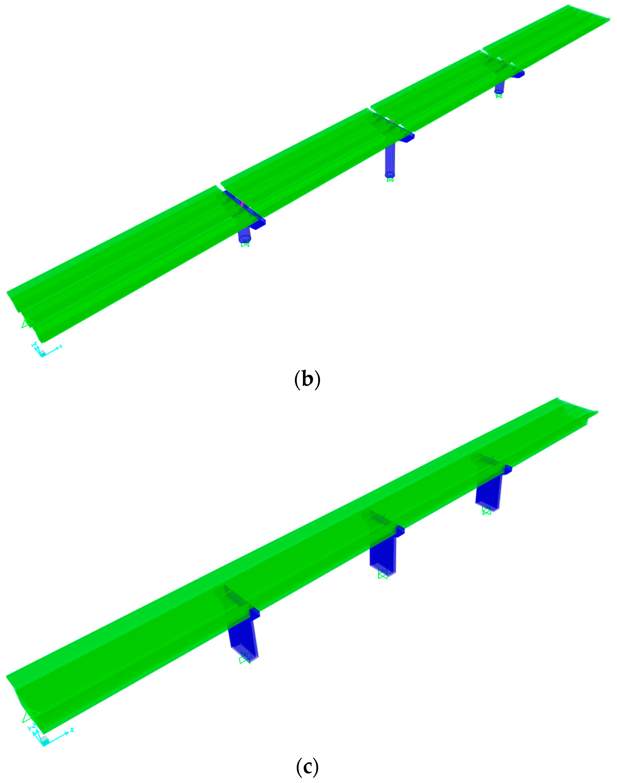
Three numerical models reproducing the geometries of the examined archetype bridges were implemented in SAP2000 v23.1.0 software [53]. The x axis of the models coincides with the longitudinal direction of the bridge, the y axis with the transverse direction, and the z axis with the vertical direction (Figure 14).

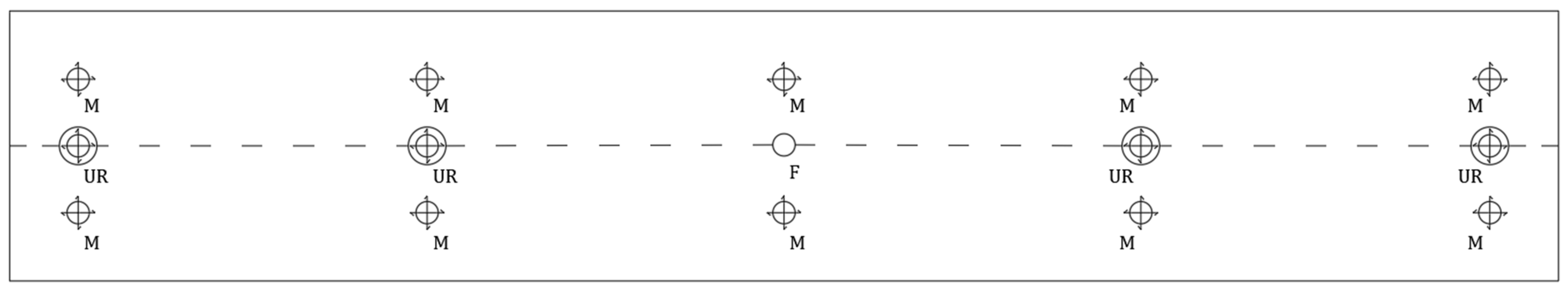
The piles were rigidly fixed to the ground; permanent non-structural loads and variable loads were uniformly distributed on the deck. For the sake of simplicity, the connections between the deck and the substructures (piles and abutments) were modeled through rigid links [53], either fixed (with no displacement) or unrestrained (free to move with no reaction) in one or two horizontal directions according to the bearing layout shown in Figure 3 for Bridges 1 and 2. Regarding Bridge 3, it was assumed that the shear keys were engaged during the earthquake, and all the axes were modeled as fixed. All links allowed free rotation about the transverse bridge axis (y-axis), while rotations about the longitudinal and the vertical bridge axes were locked. No damping was assigned to the rigid links since conventional bridge bearings are not designed to dissipate energy. The abutments were not explicitly included in the model, as they were assumed to be infinitely rigid.

The internal structural damping was modeled as Rayleigh damping [54], with parameters assigned to achieve a 5% damping ratio at the first frequencies in the longitudinal and the transverse directions. The formulation consists of the superposition of a mass-proportional damping contribution and a stiffness-proportional damping contribution and has the main advantage that there is no need to explicitly build and store a damping matrix because mass and stiffness matrices are already stored for other purposes [54]. Rayleigh damping parameters assigned in the model are summarized in

Table 5. Rayleigh damping parameters.

Parameter	Bridge 1	Bridge 2	Bridge 3
T1x [s]	0.424	0.967	0.2888
T1y [s]	0.189	0.488	0.1745
a	0.9578	0.4318	1.3562
b	0.00214	0.00516	0.00173

T_1x = fundamental period in x direction; T_1y = fundamental period in y direction; a = mass-proportional coefficient; b = stiffness proportional coefficient.

.

4.1. Material Behavior

Different material behaviors were formulated in the models depending on the examined analysis procedure. For linear procedures (ESA, RSA, LTHA), the materials were modeled as purely elastic; for nonlinear analyses (MPA, NLTHA), the nonlinear constitutive laws of C25/30 and FeB44k were implemented into the model. Whichever the adopted behavior, material characteristics were assigned as design values, calculated from the characteristic values by means of the partial factors recommended by IBC [2] (γ_c = 1.5 for concrete and γ_s = 1.15 for steel, respectively). The reduction in the stiffness of concrete members was disregarded. Structural and non-structural masses and 20% of traffic loads were considered for eigenvalue analysis (IBC [2], §5.1.3.12).

In the RSA and ESA, in accordance with IBC [2] Table 7.3.II, for fixed piles a behavior factor q = 1.5 was assumed equivalent to the maximum allowed value for RC bridges designed for low ductility class.

For linear analyses, the piles were modeled as linear elastic members. In nonlinear analysis, in order to account for inelastic concrete deformation, at the base of each pile a bidirectional plastic hinge (parametric P-M2-M3) formulated according to Table 10-8 (concrete columns) of ASCE 41-13 [55] was implemented, with the plastic hinge backbone computed accounting for the vertical load. Cyclic degradation of the moment–rotation curve was disregarded. Only for Bridge 1 was a second plastic hinge introduced at the head of the pile shafts in the transverse direction of the bridge; the frame piles may provide an additional plastic resource in this position [56].

The brittle behavior of the piles was considered by introducing hinges with rigid brittle behavior in the two main shear directions, with limits defined accounting for the shear resistance of each type of section.

Foundations and abutments were modeled as rigid constraints, and the relevant damping was neglected. This modeling assumption was aimed at locating the sources of material nonlinearity in a few members (the piles) and facilitating the comparison between the different analyses, making it easier to search for the causes of the divergence of results. Moreover, the assumption of rigid foundations is justified by past bridge design practice, where foundations were generally conservatively designed [57].

4.2. Analyses

Eigenvalue analysis was performed with a Ritz vector solution, considering a maximum of 100 modes.

Table 6. Significant modes for the three bridges.

	Bridge 1				Bridge 2				Bridge 3
Mode	T [s]	MX [%]	MY [%]	Mode	T [s]	MX [%]	MY [%]	Mode	T [s]	MX [%]	MY [%]
1	0.42	24%	0%	1	0.97	25%	0%	1	0.29	0%	60%
2	0.42	24%	0%	2	0.49	0%	62%	3	0.18	53%	0%
3	0.42	24%	0%	3	0.45	25%	0%	8	0.04	24%	0%
4	0.19	0%	84%	4	0.45	25%	0%	11	0.02	0%	19%
6	0.07	0%	2%	6	0.14	0%	5%	13	0.02	13%	0%
11	0.03	0%	10%	9	0.05	0%	5%	14	0.01	0%	16%
17	0.02	6%	0%	10	0.05	10%	0%
18	0.02	6%	0%	16	0.03	0%	13%
19	0.02	6%	0%	21	0.02	0%	5%

T = period; M_x = participating mass in x direction; M_y = participating mass in y direction.

illustrates, for each bridge, the modes that involve more than 5 percent of the total mass.

NLTHA was performed considering all modes and carrying out direct integration with the Hilber–Hughes–Taylor (HHT) method. This is an implicit method that allows for energy dissipation and second-order accuracy (which is not possible with the regular Newmark object).

For linear dynamics analyses (LTHA and RSA) all modes were considered as well. LTHAs were performed with the Modal solution and RSA using the CQC Modal combination. In accordance with the provision of IBC [2], §3.2.3.5, for RSA the approximate nonlinear strength demand was estimated by reducing the full elastic seismic demand by means of a behavior factor q = 1.5, equal to the value allowed for RC bridges designed for low ductility class according to IBC [2].

The modes to be considered for MPA were selected by analyzing the results of the eigenvalue analysis. The two simply-supported bridges (Bridge 1 and Bridge 2) showed decoupled behavior between modes in the longitudinal bridge direction, while the coupling of modes occurred in the transverse direction. The continuous-deck Bridge 3 showed modal coupling in both directions. Based on the eigenvalue analysis, three modes in the x-direction and one in the y-direction were considered for Bridge 1, and three modes in either direction were considered for Bridge 2 and Bridge 3. Pushover analyses were run with a modal lateral force pattern for each mode, and the resulting capacity curves were then converted into the equivalent bilinear curve of the equivalent single-degree-of-freedom (SDOF) system, considering post-yielding stiffening behavior. This way, a set of Capacity Spectrum Curves (CSC) for each single degree of freedom (SDOF) was obtained from the original multi-degree of freedom system. Then, the peak response of each SDOF system (corresponding to a single mode) in terms of forces and displacements was calculated from the response spectrum in accordance with the Method B of the Commentary to IBC [47] §C7.3.4. For MPAs characterized by decoupled modes, performance points were defined separately for each individual mode (which typically involved a single pile), and reaction values associated with each of them were extracted. For analyses with coupled modes, performance points were defined for each mode; reactions at the performance point were calculated and then combined according to the SRSS rule. For the sake of brevity, this procedure is not described in detail in this paper, but interested readers are referred to reference [58]. For all case study bridges, it was checked that the total mass of the pile is less than 20% of the tributary mass of the deck, and in the case of piles carrying simply supported spans (Bridges 1 and 2) no significant interaction between piles is expected; therefore, the conditions for applicability of ESA [4] were met. ESA was performed according to the individual pier model [2,24] considering a single pile and the tributary mass of the deck and assessing the response in the longitudinal and transverse directions of the bridge separately. In the longitudinal direction, for simply-supported Bridge 1 and Bridge 2, it was assumed that the width of the expansion joints between adjacent decks was larger than the seismic displacement of the individual decks (i.e., no pounding occurred), allowing the use of the single pier model also in this direction. For the continuous-deck Bridge 3, the analysis was performed considering the whole bridge as consisting of several subassemblies (the piles and the abutment) forming an in-parallel system. Also, in the case of ESA, forces and moments were estimated by reducing the full elastic spectrum by the behavior factor q = 1.5, while the displacement demand was amplified by a ductility factor which depends on the behavior factor q and the first vibration period of the bridge in either horizontal direction according to the procedure recommended by IBC [2] §7.3.3.

4.3. Costs

In terms of the costs of the seismic analyses, three budget items could be identified: modeling, computation, and output. Modeling cost includes the time requested to code the geometric and mechanical properties of the structure into the numerical model and the definition of the seismic input. The computational cost is related to the time required for the processor to perform the analysis. The cost for output is related to the time and effort required to process the data provided by the procedure to obtain the Engineering Demand Parameters (EDPs) of interest.

The computer time required for dynamic analysis depends on the size of the structure and the strength of the ground motion (stronger motions cause more nonlinear behavior, which usually increases the computer time), as well as on the computing capacity of the processor. Therefore, in order to provide information of general validity, the cost of the analysis will be discussed in qualitative terms.

Modeling nonlinear behavior in NLTHA and MPA requires a large effort that is not requested in linear dynamic procedures and ESA; similarly, modeling ground motion time history inputs in NLTHA and LTHA is more onerous than modeling the seismic input through the response spectrum (MPA, RSA and ESA). The computational cost of NLTHA is higher than that of LTHA and MPA, while RSA and ESA have practically negligible costs. Finally, calculating EDPs from the raw output of NLTHA and LTHA is very expensive, like for MPA, due to the huge number of output information provided, while for the RSA and ESA, the calculation of EDPs is straightforward.

By associating qualitative scores with the three budget items, it is possible to estimate an overall cost of analysis for each procedure and define the relevant ranking, as shown in

Table 7. Qualitative estimates of analysis cost of examined procedures.

Procedure	Modelling	Computation	Output	Total Cost
NLTHA	High	High	High	High
LTHA	Medium-High	Medium-Low	High	Medium-High
MPA	Medium-High	Medium-Low	High	Medium-High
RSA	Medium	Low	Low	Medium-Low
ESA	Low	Low	Low	Low

.

5. Results

In NLTHAs, the maxima of global engineering demand parameters (EDPs) such as pile base reactions and top pile displacements were calculated for each ground motion of the set of seven accelerograms, and then averaged, as prescribed in the codes [2,3].

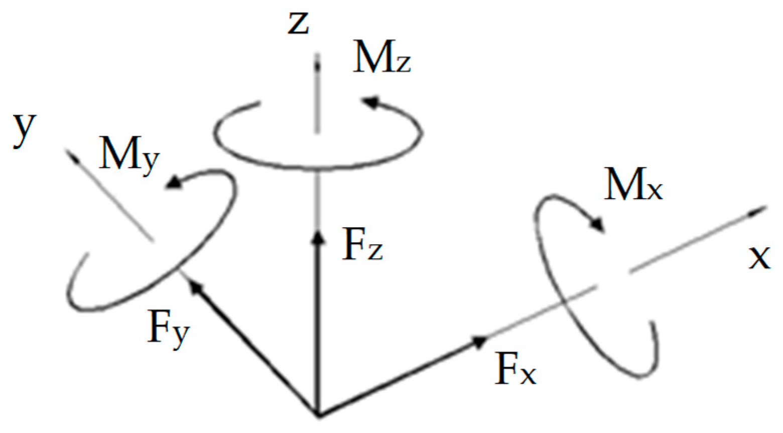
The performances of linear and nonlinear procedures were then evaluated in terms of global EDPs for each bridge, and the relative deviations from the results of NLTHA, assumed as a benchmark were calculated according to Equations (1) and (2)

$${∆}_R=\frac{R-R_{\mathrm{N}\mathrm{L}\mathrm{T}\mathrm{H}\mathrm{A}}}{R_{\mathrm{N}\mathrm{L}\mathrm{T}\mathrm{H}\mathrm{A}}}$$

(1)

$${∆}_U=\frac{U-U_{\mathrm{N}\mathrm{L}\mathrm{T}\mathrm{H}\mathrm{A}}}{U_{\mathrm{N}\mathrm{L}\mathrm{T}\mathrm{H}\mathrm{A}}}$$

(2)

where R_NLTHA and U_NLTHA stand for the benchmark values of pile base reactions (forces, F, and moments, M) and top pile displacements calculated from NLTHA, and R and U denote the corresponding values provided by the procedure under examination. Pile base reactions are defined in accordance with Figure 15, where the x-axis is aligned to the longitudinal direction of the bridge, and the y-axis to the transverse direction.

The EDPs calculated from the analyses for the three case studies are reported and commented on in the following subsections; tabulated deviations from the benchmark are reported in Appendix B.

5.1. Bridge 1

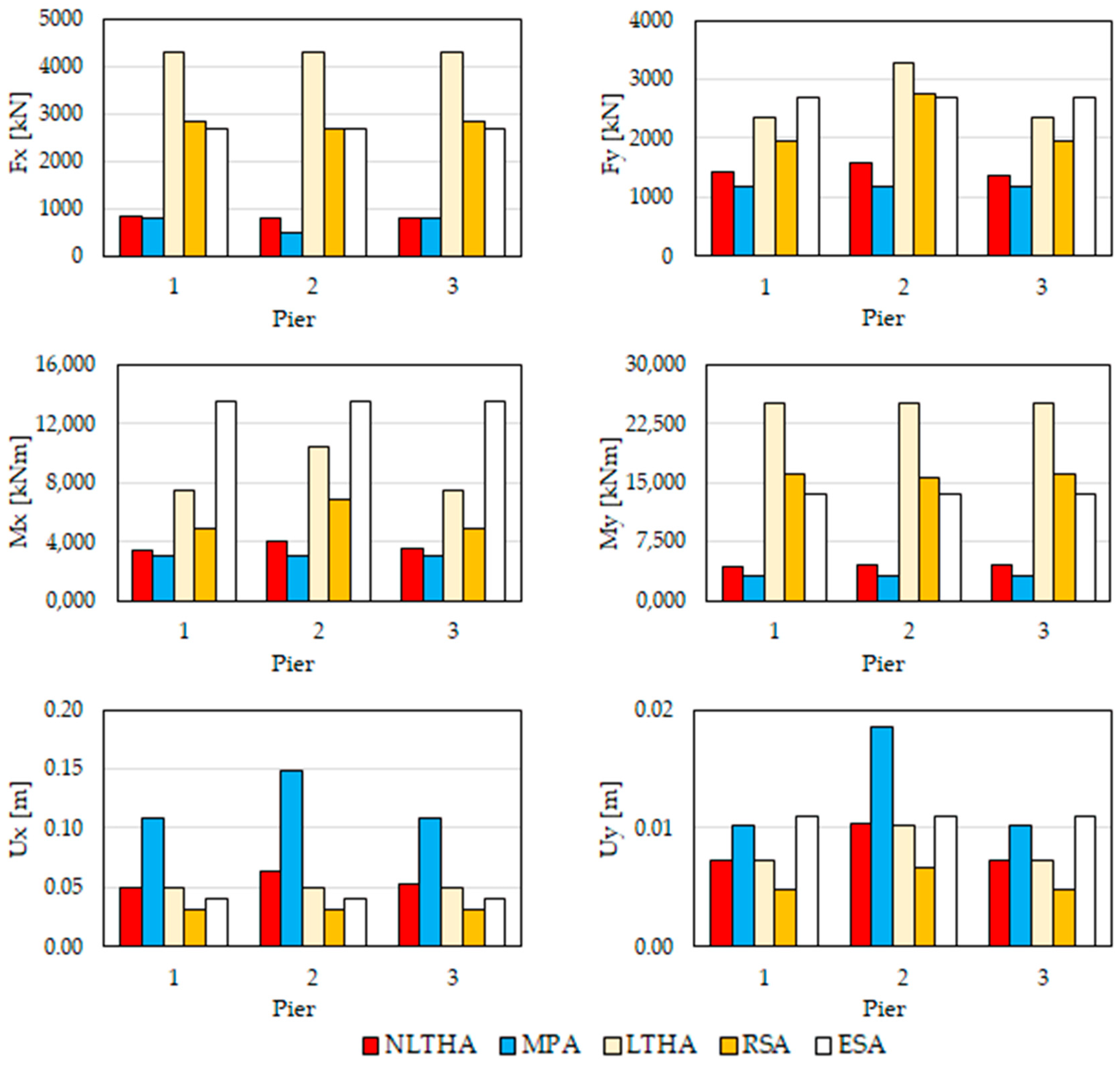
The results in terms of EDP of the analyses conducted on Bridge 1 are shown in Figure 16, Figure 17 and Figure 18 for the three seismic scenarios; Figure 19 reports the maximum absolute deviation from the benchmark for each EDP obtained from the simplified analyses as a function of the PGA.

Considering linear procedures, some points are worth noting.

First, linear procedures overestimate base reactions in the longitudinal direction of the bridge (F_x and M_y), with deviations from the benchmark that increase as the seismic intensity does (maximum deviation of approximately +450% on pile P2 for LTHA, +250% on pile P3 for RSA and +240% on pile P2 for ESA in zone 1). This behavior is due to the fact that the forces and moments calculated in NLTHA are capped because of material nonlinearities, while in linear analyses the forces and moments are not bound and increase almost proportionally with the magnitude of the seismic action. In NLTHA, plastic hinges were activated at the bases of each pile in seismic zones 1 and 2, while in seismic zone 3 plastic hinges were not triggered in piles P1 and P3. Therefore, at lower intensities of seismic input, the material nonlinearities are less engaged and the deviation of the linear analyses from the benchmark is reduced (maximum deviations on the order of +80% for LTHA, +45% for MPA and +50% for ESA in seismic zone 3).

The performance of linear procedures is better when the goal is to estimate the base reactions in the transverse bridge direction (F_y and M_x). This is explained considering the frame piles of Bridge 1 have a higher elastic capacity in the transverse than in the longitudinal direction (the moment at first yielding is about 2.5 times larger, as shown in Table 4). LTHA provides maximum deviations on F_y and M_x from the benchmark on the order of +160% in zone 1, +80% in zone 2 and +17% in zone 3. On the other hand, corresponding maximum deviations of RSA in the three seismic zones are +75%, +25% and -30%, respectively. Both LTHA and RSA have similar accuracy in estimating forces and moments. On the contrary, ESA shows a better performance in predicting the forces (with deviations similar to those of RSA), but worse accuracy on the moments.

In general, RSA shows better accuracy than LTHA as a consequence of the different models of seismic demand assumed in either analysis. The accelerograms used in LTHA referred to the elastic spectrum, while in RSA the design spectrum was defined by assuming the maximum behavior factor q = 1.5 allowed for RC bridges designed for low ductility class in accordance with IBC [2] Table 7.3.II. It was separately checked (results have not been reported for the sake of conciseness) that disregarding the behavior factor, RSA would provide the same results as LTHA. Though very simple, ESA provides acceptable estimates of F_y in seismic zones 2 and 3, and of M_x in seismic zone 3. The deviations are larger on F_x (three times larger than on F_y in zones 1 and 2) because of material nonlinearities triggered in the weakest direction of the frame pile.

Base reactions calculated from MPA are in acceptable agreement with the benchmark values, which is due to the common capped material behavior assumed in both NLTHA and MPA. Accuracy is similar on both forces and moments, regardless of the considered bridge direction, and there is not an apparent influence of the seismic intensity. The maximum deviations on the estimated reactions are about −37% (on F_x, pile P2) in zone 1, −24% (on F_x, piles P1 and P3) in zone 2, and −35% (on F_y and M_x, piles P1 and P3) in zone 3. In this regard, it is worth noting that MPA underestimates the reactions calculated by NLTHA. This result is specifically related to the ductile behavior exhibited by Bridge 1, characterized by capacity curves with a softening branch: beyond the maximum point, the strength decreases as the displacement demand increases; since MPA overestimates the displacements, the base reactions are lower than those predicted by nonlinear time history analyses.

The performance of linear procedures for the calculation of top pile displacement is substantially better, especially in medium-high and high seismicity scenarios, where the relative deviations from the benchmark are one-fold or two-fold smaller than those for base reactions. LTHA provides conservative estimates of the displacements in the medium-low and medium-high seismicity zones, with deviations that tend to become negligible in seismic zone 1 (Reggio Calabria). RSA always underestimates the displacements in both the longitudinal and transverse bridge directions. This effect is ascribed to the assumed behavior factor q = 1.5, which leads to overestimating the contribution to damping of the plastic deformation at the base of the piles. In this regard, it is recalled again that for LTHA, the set of accelerograms was selected in order to match the elastic design spectrum, disregarding the behavior factor q which on the contrary was considered in RSA and ESA.

The longitudinal displacement U_x calculated by MPA in the high and medium-high intensity scenarios is one order of magnitude higher than the benchmark value, while the deviation is smaller for the transverse displacement U_y, and practically in line with the deviations provided by linear procedures. In the medium-low seismic scenario, the accuracy of MPA on both U_x and U_y is similar to those of LTHA and RSA.

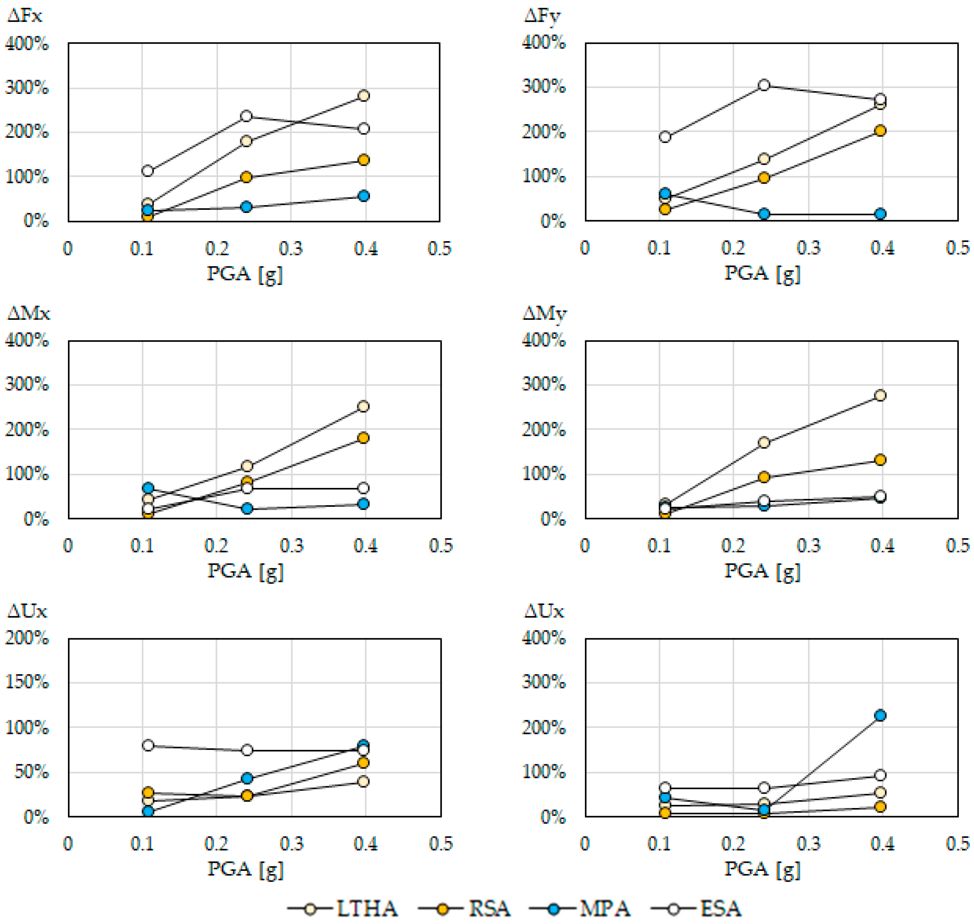
Eventually, the diagrams in Figure 19 provide a clearer visualization of the performance of the examined procedures in the different seismic scenarios. For the simple-supported Bridge 1, accurate estimates of the base reactions whichever the intensity of the seismic scenario, are provided only by MPA; the use of linear methods should be limited to the case of moderate-low intensity earthquakes. On the contrary, displacements on the top of the piles are better calculated by linear analyses, with the best accuracy in the high-seismicity scenario provided by LTHA.

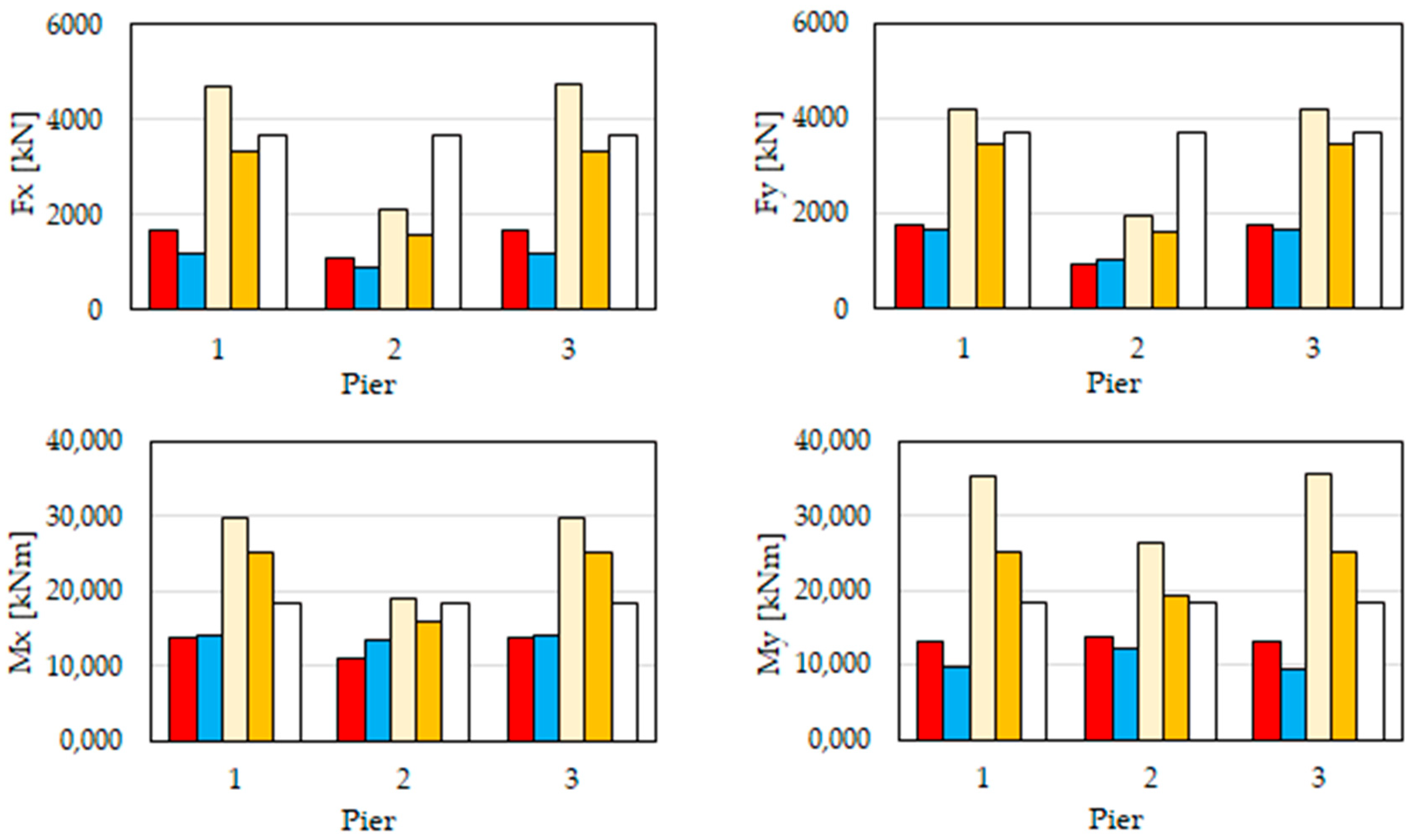
5.2. Bridge 2

The results in terms of EDP of the analyses conducted on Bridge 2 are shown in Figure 20, Figure 21 and Figure 22, considering the three seismic scenarios separately. Figure 23 reports the maximum absolute deviation from the benchmark for each EDP as a function of the PGA.

Linear procedures provide poor estimates of base reactions, though with lower deviations from the benchmark than those observed for Bridge 1. The deviation increases again with the intensity of the earthquake, reaching values as high as +280% for LTHA and up to +200% for RSA in zone 1. Since the piles have the same cross-sectional properties in both the x and y axes, the performance of the analyses is similar in either direction. In the medium-low seismicity scenario, the deviations are fair, between 30 and 50% for LTHA, and less than 20% for RSA (but for a 27% deviation on F_y on pile P2). ESA calculates acceptable estimates of the moments for each considered seismic scenario, while the forces are affected by larger errors, especially the forces on pile P2 (this is apparent in zones 2 and 3). In NLTHA yielding occurred at the bases of all piles in the bridge in seismic zone 1, while in seismic zones 2 and 3 pile P2 remained in the elastic range as it was designed with a higher amount of longitudinal reinforcement. This explains the better accuracy of linear techniques in moderate-intensity seismic scenarios.

MPA provides the smallest deviations on base reactions, though benchmark values are underestimated by more than 50% in seismic zone 1 (−57% and −52% on F_x on piles P1 and P3). As already observed for Bridge 1, Bridge 2 exhibits a ductile behavior, with capacity curves associated with the first three modes with a softening branch: since MPA calculates larger displacements of the structure than NLTHA, the associated base reactions are lower, especially in the longitudinal direction of the bridge. The accuracy on F_x and M_y improves in zones 2 and 3 where the seismic forces are lower. The opposite trend is observed on F_y and M_y on pile P2, where the reactions are overestimated.

The accuracy of LTHA and RSA in terms of top pile displacements is acceptable in zones 2 and 3 where the deviation of the structural response from linearity is small. In particular, the predictions are better for piles P1 and P3 than for P2. However, while LTHA overestimates the benchmark values, RSA underestimates the displacements in both longitudinal and transverse directions due to the effect of the behavior factor q = 1.5. The performance of ESA is comparable to the one of RSA in zone 1, but less accurate in zones 2 and 3. In particular, the deviation is higher on pile P2 which is ascribed to the fundamental period of the tall pile combined with the shape of the target spectrum.

MPA shows a worse performance in terms of displacements. The top pile displacements are overestimated, with maximum deviations of about 80% on U_x, and up to 225% on U_y for pile P2 in the high-intensity seismic scenario. The deviations become acceptable, and in line with those observed for LTHA and RSA, in zones 2 and 3.

Figure 23 shows that, like in the case of Bridge 1, the most accurate estimates of the base reactions for every seismic zone are provided by MPA, while the linear methods are accurate for moderate-low seismicity scenarios that do not substantially engage the plastic resources of the structure. RSA and ESA show better performance than LTHA as they partially account for the anelastic response of the piles through the behavior factor q. It is worth noting for the particular bridge that fair estimates of the base moments M_x and M_y are calculated by ESA.

LTHA, RSA and MPA provide comparable accuracy in estimating the longitudinal displacement of the pier cap for moderate-low and moderate-high earthquakes; the accuracy becomes lower for high seismicity. Similar results are obtained for the transverse displacements.

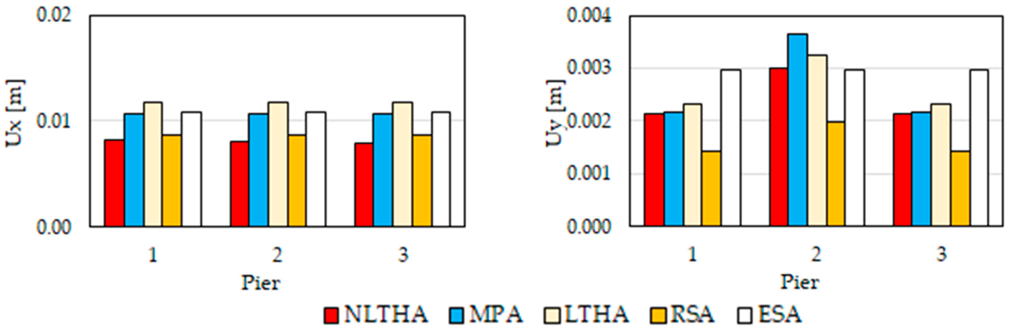
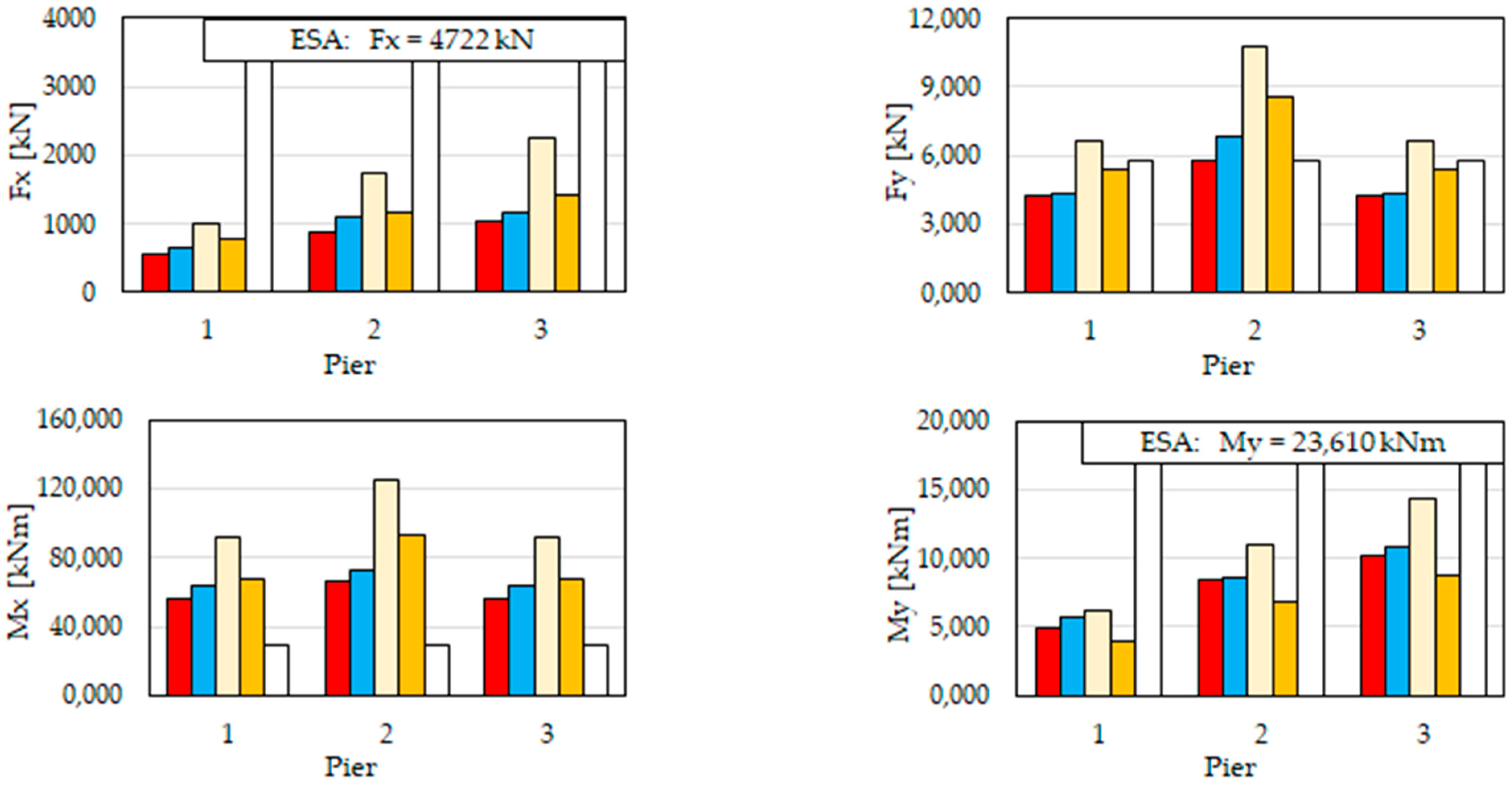
5.3. Bridge 3

The results of the analyses conducted on Bridge 3 are shown in Figure 24, Figure 25 and Figure 26 in terms of EDP, considering the three seismic scenarios separately, and in Figure 27 as the maximum absolute deviation from the benchmark for each EDP as a function of the PGA.

Regardless of the seismic scenario, ESA provided estimates of base reactions and top pile displacement along the longitudinal direction of the bridge (F_x, M_y, U_x, respectively) that were one order of magnitude greater than the values provided by the other procedures. Such behavior can be explained by recalling that in ESA each pile is studied individually, considering only its own mass and stiffness and the tributary mass of the deck according to the individual pier model [24], and as a fact, the bridge is modeled as if it consisted of simply supported spans. On the contrary, in a continuous-deck bridge, an in-parallel system, in which the piles resist the horizontal seismic actions depending on their stiffnesses, is triggered. Since the stiffness of the assumed hollow pile is very high, its base reactions evaluated according to ESA are very high too. For the sake of clarity, the results of ESA in terms of F_x, M_y, and U_x have not been drawn in the diagrams but reported only as a value.

In the transverse direction, the estimates provided by LTHA and RSA improve their accuracy as the seismic intensity decreases, with deviations (in absolute value) less than 20% for RSA and less than 50% for LTHA in the moderate-low scenario. In the longitudinal direction, both LTHA and RSA show the lowest deviation from the benchmark in zone 2, highlighting that in the continuous-deck bridge configuration, the influence of the ground motion intensity is less apparent than in the simply supported bridges. In general, the performance of RSA is better than that of LTHA; RSA overestimates base reactions up to +77% in the highest seismic scenario, but its accuracy improves significantly in zone 2 and zone 3, where it may represent a viable procedure to estimate the seismic response of the continuous-deck bridge at a low computational cost. The accuracy of linear analyses is significantly better for Bridge 3 than for Bridge 1 and Bridge 2, as inferred from tabulated deviations in Appendix B, due to the high elastic strength of the rectangular hollow section of the piles (Table 4).

Both LTHA and RSA provide fair estimates of the top pile displacements, though they show opposite behavior: LTHA overestimates the displacements, with a maximum deviation of 20%, while RSA is conservative, with deviations ranging between −20% in seismic zone 1 scenario and −30/−35% in seismic zones 2 and 3. The different performance between LTHA and RSA is ascribed again to the behavior factor q = 1.5 assumed in RSA. ESA provides deviations on the order of 50% on the transverse displacements, but unrealistic estimates of the longitudinal displacement as it relies on the assumption of the individual pile model.

MPA calculates a reliable estimate of base reactions, with maximum deviations less than 40%; there is no apparent influence of the seismic scenario on the accuracy. Different from the case studies of Bridge 1 and Bridge 2, for the continuous deck Bridge 3, the analysis overestimates forces and moments at the pile bases, resulting in a conservative approach. Unlike the bridges examined in Section 5.1 and Section 5.2, Bridge 3 exhibits a brittle behavior (for the second and third modes the structure fails in shear), and therefore, the base reactions are related to the displacement demand by a relationship of proportionality. Indeed, as shown in Figure 24, Figure 25 and Figure 26, base reactions and displacement follow the same general trend. Regarding the reliability of displacement estimates, deviations from the benchmark range between about 20% in seismic zone 2, and more than 100% in seismic zone 1 for U_x, and increase from 0% in seismic zone 1 to about 270% in seismic zone 3 for U_y.

It must be emphasized that, differently from Bridge 1 and Bridge 2, Bridge 3 has a continuous-deck layout with seismic restraints on the bearings, and the effects of seismic actions are shared between the piles: in the longitudinal direction of the bridge base reactions F_x and M_y, and top pile displacements increase from Pile 1 to Pile 3. This behavior is reproduced by every procedure but for ESA.

Figure 27 shows that in the continuous-deck bridge, the most accurate estimates of base reactions are provided, as expected, by MPA, but RSA allows obtaining, at a lower cost, predictions with errors less than 50% in seismic zones 2 and 3, and up to 75% in seismic zone 1. Only M_y linear and nonlinear analysis provide similar results while, in general, it is necessary to perform a nonlinear analysis to obtain acceptable previsions of the structural response. Noteworthy, in the transverse direction the accuracy of base reactions calculated by ESA is similar to that assessed for RSA, but in the longitudinal direction, ESA provides unrealistic estimates and the relevant deviations were not reported in the diagram as out of range. By comparing the diagrams of Figure 27 to those of Figure 19 and Figure 23, it is apparent that the average error of NLTH and RSA is smaller for Bridge 3, which is explained as a consequence of the high elastic capacity of its piles, which prevents, or reduces the engagement of nonlinearities in the material behavior. Concerning the displacements, the results of linear analyses are quite fair regardless of the seismic scenario, while the performance of MPA deteriorates with increasing seismic intensity, resulting in unacceptable deviations in the high seismicity situation.

5.4. Main Limitations

The study has considered the cases of RC bridges with straight decks. Other typologies of bridges, differing in materials (e.g., steel, masonry, or composite bridges), layout (e.g., curved bridges), and dynamic properties (e.g., flexible bridges with a long fundamental period), as well as bridges provided with seismic isolation or supplementary energy dissipation devices, have not been investigated. Therefore the validity of the results applies only to the specific typology addressed in the paper. For example, bridges with a fundamental period longer than 2 s are expected to provide an essentially elastic response to ground motions even of high intensity, and therefore, it is likely that linear procedures will provide a better performance in comparison to the results of the present study, where bridges with a period between 0.25 and 1.0 s in the longitudinal direction, and between 0.15 and 0.5 s in the transverse direction were examined.

Therefore, further investigations are needed to confirm or update the findings of the study to other bridge configurations.

6. Conclusions

The paper investigates the reliability of procedures recommended by the Italian Building Code [2] and the Eurocode [3,4] for the analysis of ordinary bridges subjected to seismic actions through their application to three archetype multi-span bridges, representative of geometric features and bearing layouts typical of the Italian bridge stock. Specifically, Bridge 1 is a simply supported bridge characterized by frame piles with different stiffness and capacity in the two horizontal directions; Bridge 2 is another simply supported bridge with three piles of different heights and different capacities, though the behavior of each pile is identical in the two horizontal directions; Bridge 3 represents the case of a continuous-deck structure on multiple piles, where the piles have a very high elastic capacity.

The main results of the study are summarized in the next points:

• Linear techniques such as LTHA and RSA are characterized by the low cost of analysis but, in general, their accuracy in estimating base reactions is low, especially in high-intensity seismic scenarios, with huge deviations from the benchmark values provided by NLTHA; such behavior is a consequence of the inability of the linear modeling to account for the capping in strength associated to nonlinear material behavior. In contrast, nonlinear material behavior can be formulated in MPA which, therefore, provides the most accurate estimates of forces and moments at the base of the piles.
• Due to the reason mentioned above, i.e., the inability to capture the capped strength response of the materials, the reliability of linear analyses (LTHA and RSA) for the calculation of base reactions is higher in those situations where the behavior of the bridge has small deviations from linearity, i.e., in case of medium-low or low-intensity seismic scenarios, and/or substructures with high elastic strength; in the case of piles with different behavior in the two horizontal directions, the accuracy of linear analyses is consequently different depending on the considered direction.
• MPA provides acceptable estimates of base reactions and top pile displacements of both simply-supported and continuous-deck bridges, with an accuracy apparently independent of the ground motion intensity. In the examined case studies, base reactions were estimated in the simply-supported bridge configuration due to the ductile behavior of the bridge represented by capacity curves with a post-peak softening branch (by which the base reaction decreases as the displacement demand increases), and overestimated in the hyperstatic continuous-deck bridge configuration with massive piles, characterized by a brittle behavior and an almost proportional relationship between base reactions and displacement of the control point.
• Linear procedures seem to be more accurate than MPA for estimating the displacements on the top of the piles, especially in high-seismicity scenarios, where the solution provided by MPA substantially deviates from the benchmark.
• For simply-supported bridges, the performance of ESA is comparable to that of the other linear procedures, but at a substantially lower cost. For the continuous-deck bridge, ESA provides reliable estimates of base reactions and top pile displacements in the transverse bridge direction, where the individual pier model applies; on the contrary, in the longitudinal bridge direction, ESA provides unrealistic values of base forces and moments as it is not able to catch the actual behavior of the piles that form an in-parallel system in which the piles resist to the horizontal seismic actions depending on their stiffnesses.

From a practical point, the study suggests that ESA can be a useful tool for the preliminary assessment at the portfolio scale of the seismic vulnerability of multi-span, simply-supported bridges, leaving more accurate but more expensive nonlinear analyses to the in-depth assessment of identified high-risk structures. Similarly, RSA provides the best trade-off between cost and accuracy for ordinary structures that remain in the elastic range or are subjected to limited anelastic deformations (e.g., structures subjected to weak or moderate-weak earthquakes, or resting on strong piles). LTHA is not recommended due to the large analysis cost without a substantial improvement in accuracy. MPA should be considered as a viable alternative to NLTHA for the assessment of individual critical bridges where a high level is required, though, as highlighted in the study, care should be paid to possible underestimates of actual reactions in simply supported bridges.

The paper is mainly addressed to practitioners involved in the seismic assessment of bridges, who must face the problem of choosing the most appropriate technique of analysis in compliance with the codes. Though the results are restricted to the simple cases of bridges with straight decks shown in the paper, the Authors deem that the work has some merit as it provides, for some common bridge typologies, a comparative evaluation of some of the most popular analysis methods, pointing out their main strengths and limitations.