Failure Probability and Economic Loss Assessment of a High-Rise Frame Structure under Synthetic Multi-Dimensional Long-Period Ground Motions

Abstract

Multiple research studies and seismic data analyses have shown that multi-directional long-period ground motion affects crucial and intricate large-scale structures like oil storage containers, long-span bridges, and high-rise buildings. Seismic damage data show a 3–55% chance of long-period ground motion. To clarify, the chance of occurrence is 3% in hard soil and 83% in soft soil. Due of the above characteristics, the aseismic engineering field requires a realistic stochastic model that accounts for long-period multi-directional ground motion. A weighted average seismic amplification coefficient selected NGA database multi-directional long-period ground motion recordings for this study. Due to the significant low-frequency component in the long-period ground motion, this research uses empirical mode decomposition (EMD) to efficiently decompose it into a composite structure with high- and low-frequency components. Given the above, further investigation is needed on the evolutionary power spectrum density (EPSD) functions of high- and low-frequency components. Analyzing the recorded data will reveal these functions and their corresponding parameters. Proper orthogonal decomposition (POD) is needed to simulate samples of high- and low-frequency components in different directions. These samples can be combined to illustrate multi-directional long-period ground motion. Representative samples exhibit the seismic characteristics of long-period multi-directional ground motion, as shown by numerical examples. This proves the method’s engineering accuracy and usefulness. Moreover, this study used incremental dynamic analysis (IDA) to apply seismic vulnerability theory. This study investigated whether long-period ground motions in both x and multi-directional directions could enhance the seismic response of a high-rise frame structure. By using this method, a comprehensive seismic economic loss rate curve was created, making economic loss assessment clearer. This study shows that multi-directional impacts should be included when studying seismic events and calculating structure economic damages.

1. Introduction

With the advancement of economic and social development, there has been a noticeable increase in the construction of large-scale infrastructure projects that include intricate systems. These projects include high-rise buildings, long-span bridges, gymnasiums, and oil storage tanks, among others. It is important to note that these structures are susceptible to the effects of long-period ground motion [1]. The substantial attention and emphasis of engineering and academia have been directed to multi-directional long-period ground motion due to the present advancements in anti-seismic design theory, the renewal of design concepts, and the increased availability of measured records. The foundation for ensuring the safety and reliability of large-scale infrastructure lies in anti-seismic design and analysis, which are conducted by considering the appropriate external excitation input of multi-directional long-period ground motion. Nevertheless, in the field of engineering structural dynamic time history analysis, it is common practice to utilize measured records as external excitations. However, these records are often limited in quantity and may not always accurately represent the soil conditions and seismic environment in which the infrastructure is situated. Given the aforementioned facts, it is crucial to thoroughly examine and accurately depict the seismic attributes of multi-directional long-period ground motion. Subsequently, it is imperative to develop a sound stochastic model in order to facilitate anti-seismic analysis.

The establishment of a realistic stochastic model relies on a thorough investigation of the seismic features of multi-directional long-period ground motion. The initial recorded long-period ground motion data were obtained in Tokachi-Oki in 1968. Subsequent research has revealed that long-period ground motion typically comprises two distinct spectrum components: body waves and surface waves. Body waves primarily consist of high-frequency components, while surface waves are characterized by low-frequency components [1]. Numerous researchers have conducted extensive investigations on these two types of components, focusing on three key seismic characteristics: spectrum, duration, and energy. A comprehensive investigation was undertaken by Yang [2] to examine the long-period ground motion resulting from the CHICHI and Northridge earthquakes. The study focused on utilizing suggested indicators, such as the period of Hilbert marginal spectrum and the improved characteristic period, to describe the seismic characteristics of the spectrum. Additionally, the analysis aimed to determine the extent to which these indicators accurately depict the high- and low-frequency properties of long-period ground motion. In a study conducted by Maeda [3], an investigation was carried out on the seismic features of long-period ground motions resulting from the 2003 Tokachi-Oki earthquake occurrences. The findings of this study proposed the utilization of peak ground velocity (PGV) as an indicator for differentiating between normal ground motion and long-period ground motion. In their research, Kitamura [4] examined the impact of the spectrum and energy of long-period ground motion on the dynamic response of structures. The study focused on the seismic occurrences of the 2011 earthquake off the Pacific coast of Tohoku and the 2003 Tokachi-Oki earthquake. Chen [5] conducted a calculation of the local spectrum density for the measured long-period ground motion and subsequently examined the energy distribution features within the low-frequency range of said ground motion. In broad terms, when comparing normal ground motion to long-period ground motion, the distinction can be succinctly described as follows: long-period ground motion exhibits energy distribution across both the low- and high-frequency ranges of the spectrum, possesses a longer duration, and demonstrates a lower peak ground acceleration [6]. Numerous researchers prioritize the investigation of seismic features pertaining to long-period ground motion. However, the current body of research lacks a specific quantification of energy distribution in the time–frequency domain of long-period ground motion, which is crucial for a comprehensive understanding of the seismic characteristics of such ground motions in engineering applications. Therefore, it is imperative to develop a suitable model and determine the appropriate parameters for future investigations in this field.

In the past few decades, there has been a notable acceleration in global population growth, resulting in a significant influx of individuals into urban areas. Consequently, this has led to a scarcity of available land for urban construction, thereby impeding economic and industrial development due to increasingly stressed spatial conditions. Within this particular environment, it is evident that high-rise buildings have emerged as an indispensable preference in the realm of urban construction. In recent times, there has been a significant and quick development. Significant advancements have been achieved in the domains of overall construction, vertical elevation, stratification, and capacity. However, high-rise buildings are typical long-period structures, making them more susceptible to the low-frequency components associated with long-period ground motion activity. Based on the aforementioned understandings, a substantial number of researchers has conducted extensive research on the dynamic response and damage process of tall buildings subjected to long-period ground motions.

In their study, Chung et al. [7,8,9] conducted a vibration table test on an 80 m high-rise frame structure at the E-DEFENSE facility. The objective of their research was to investigate the seismic resistance of high-rise structures subjected to long-period ground motions. Takewaki et al. [10] examined the seismic resistance of high-rise structures with 40 floors and 60 floors in the context of the 2011 East Japan earthquake. They specifically focused on the long-period ground motion effects and cyclic loading and compared the analysis results for structures with and without damping devices, structures with single or dual damping devices, as well as the influence of a dampening device on the structural response. Masayuki Nagano [11] conducted a study on long-period ground motion activity in the Kanto and Kansai regions, focusing on the earthquakes recorded in 2011 in East Japan. In their study, Bai [12] examined the seismic performance of a pre-existing high-rise steel frame structure in Japan. The analysis was conducted by considering the far-field harmony and seismic input, specifically focusing on the structure’s response to vibrations occurring in a distant location. Liao [13] selected a 5-story and 12-story reinforced concrete framework as the subject of their investigation. The study focused on analyzing the structural response of two buildings of varying heights to long-period ground motions and normal ground motions using a non-linear time analysis. In a study conducted by Alavi [14], the authors utilized long-period ground motion as the input to analyze the dynamic characteristics of a 20-floor reinforced-concrete frame structure. In a subsequent study, Ariga [15] investigated the response of a 10-floor foundation high-rise structure subject to long-period ground motions and normal ground motions. Their findings revealed a resonance phenomenon between long-period ground motions and high-level structures in terms of fundamental seismic response. In a study conducted by Arash [16,17], the performance of a magnetorheological damper was examined as an intelligent dissipating device in isolated buildings subjected to long-period ground motions. The results indicated that an optimized semi-active control system could effectively mitigate the building’s pounding and significantly enhance its behavior in comparison to the isolated-pounding building. At certain specified gap distances, the behavior of the structure was even identical to that of the building without the pounding.

Evidently, there are two principal concerns that necessitate resolution, as indicated by the aforementioned progress in the research. First, the multi-directional characteristics of long-period ground motions are not accounted for in the current seismic economic loss assessment of structures. Furthermore, the implementation of an extrinsic incentive is significantly predicated on measured records extracted from databases, which present considerable variability and are difficult to replicate, and creates a challenge in accurately representing average engineering characteristics. In this context, the main idea of this paper is to suggest an efficient and accurate stochastic model to describe multi-directional long-period ground motion by introducing a new method. The main structure of this paper is as follows: Section 2 introduces the selection principle of multi-directional long-period ground motion. Moreover, to fully research the seismic characteristics of multi-directional long-period ground motion, the empirical mode decomposition (EMD) method is adopted in this section to decompose said motion into a superimposed form of its high- and low-frequency components. Section 3 suggests the evolutionary power spectrum density (EPSD) functions of high- and low-frequency components and the parameter identification method of corresponding power spectrum density (PSD) functions and modulating functions using a normalized energy distribution function (NEDF) and a normalized frequency domain energy distribution function (NFEDF). As previously mentioned, the high- and low-frequency components are considered to be part of a 1D-2V stochastic vector process, and Section 4 expounds the proper orthogonal decomposition (POD)-based method for simulating them. Generally, the representative samples of multi-directional long-period ground motion can be obtained by superimposing those of its high- and low-frequency components. The accuracy of the proposed method is revealed in Section 5, and the engineering applicability of the suggested EPSD functions is verified. A typical high-rise frame structure is employed in Section 6, and its vulnerability is studied as subjected to a simulated multi-directional and x-directional ground motion. Additionally, this study proceeds to conduct a seismic failure probability and economic loss assessment based on the aforementioned analysis. Section 7 incorporates a set of concluding notes.

2. The Decomposition of Measured Records of Multi-Dimensional Long-Period Ground Motion

2.1. The Selection Principle

Recent research shows that long-period ground motion has a significant impact on large-scale structures that are provided with a longer natural period, such as high-rise buildings, long-span bridges, and oil storage tanks. In this view, the acceleration response spectrum, which can reflect the maximum acceleration response under a given ground motion, is employed in this paper as the index for selecting long-period ground motion data from a database. To this end, the weighted average seismic amplification coefficient of a measured ground motion $a(t)$, which is obtained via the acceleration response spectrum, is adopted in this paper and is defined as follows [18]:

$$\beta =\frac{{\displaystyle \sum _{m=1}^M[T_{0,m}^2(\frac{\alpha (T_{0,m})}{PGA})]}}{{\displaystyle \sum _{m=1}^M{T}_{0,m}^2}}$$

(1)

where $T_{0,m}$ indicates the m-th value of the M equidistant discrete natural periods of SDOF systems, for which the range is $[2,10]$. $\alpha (T_{0,m})$ indicates the acceleration response spectrum that correspond to $T_{0,m}$, with a structure damping ratio of 0.05. PGA indicates the peak ground acceleration of $a(t)$. Generally speaking, a ground motion with $\beta >0.3$ can be considered a long-period ground motion.

Further, the measured records of long-period ground motion with three directions are selected based on the weighted average seismic amplification coefficient and further divided into three categories according to the average shear wave velocity at the top 30 m ($V_{\mathrm{S}, 30}$), i.e., stiff or soft rock soil with $V_{\mathrm{S}, 30}>450 \mathrm{m}/\mathrm{s}$, medium–hard soil with $300 \mathrm{m}/\mathrm{s}\le V_{\mathrm{S}, 30}\le 450 \mathrm{m}/\mathrm{s}$, and medium–soft soil with $V_{\mathrm{S}, 30}<300 \mathrm{m}/\mathrm{s}$ [19,20]. Consequently, a total of 295 measured far-filed long-period ground motion records are selected; their details’ information is listed in

Table 1. The selected measured far-filed long-period ground motion records’ correspondence between site classes and $V_{\mathrm{S}, 30}$.

Measured Record	Site Classes
	1	2	3
$V_{\mathrm{S}, 30}$ (m/s)	>450	300~450	<300
Number of groups	93	72	130

.

2.2. The EMD-Based Decomposition Method

The long-period ground motions obtained both high-frequency components and significant low-frequency components and led to the non-stationary nature of their spectrum in the frequency domain. To illustrate this phenomenon, Figure 1a displays the acceleration time history of the CHICHI earthquake in three directions, as observed by station TCU029. The presence of evident non-stationary features in the frequency domain of the presented sample poses some challenges for conventional modeling methods, which are only suited for stochastic processes with stationary frequency. Because of this, it is imperative to consider long-period ground motion as a composite of high- and low-frequency components and conduct independent investigations on their respective seismic features.

This study introduces the empirical mode decomposition (EMD) approach, proposed by Huang, to decompose long-period ground motion in order to advance the aforementioned idea. In contrast to previous signal decomposition methods, the EMD approach does not require the pre-specification of any basis functions. Instead, it decomposes a signal by employing a screening procedure to obtain a sum of various intrinsic mode functions (IMFs) and a residual component. EMD can be utilized for the breakdown of various types of signals, with a special focus on non-stationary signals like ground motion. The specific decomposition process of this approach can be found in reference [21]. Figure 1b,c presents the instantaneous-frequency components (IMFs) and residual of the previously mentioned time history of the CHICHI earthquake in the x direction. The analysis reveals that, as the decomposition number increases, the frequency components exhibit a steady reduction, indicating a corresponding increase in the long-period components.

Further, the weighted average seismic amplification coefficient $\beta$ of each IMFs is calculated to determine the high-frequency IMFs and low-frequency IMFs by comparing them with 0.3. The $\beta$ of each IMFs is displayed in

Table 2. The weighted average seismic amplification coefficient of each IMFs.

	IMFs
No.	1	2	3	4	5	6	7
$\beta$	0.094	0.17	0.32	0.93	2.66	1.65	1.08

, which shows that IMF1~IMF2 and IMF3~IMF7 belong, respectively, to high-frequency IMFs and low-frequency IMFs. Hence, the superposition of IMF1 to IMF2 and IMF3 to IMF7 can achieve the goal of decomposing long-period ground motion into its high- and low-frequency components. Figure 2a shows the high- and low-frequency components of the CHICHI earthquake, and Figure 2b reveals the corresponding seismic influence coefficients. Figure 2b shows that the seismic influence coefficients of the decomposed high- and low-frequency components fit well with those of the original ground motion at the time intervals of 1~2 s and 2~10 s, respectively. Further clarification is required regarding the fact that Figure 2b reconstructs ground motion by summing all the IMFs and provides a comparison with the original ground motion. This comparison serves as additional evidence supporting the assertion that the EMD method does not introduce any modifications into the original signal. In light of this, the investigation and modeling of high- and low-frequency components of multi-directional long-period ground motions can be undertaken in the following work.

3. The EPSD Functions of Multi-Directional Long-Period Ground Motion

3.1. The EPSD Model

In this paper, we only take non-stationary intensity measurements of the high- and low-frequency component processes in the u direction $X_i^u(t)$ into consideration for simplicity, and the corresponding evolutionary power spectrum density (EPSD) functions $S(\omega ,t; {\mathsf{\lambda }}_{S_i}^u)$ can be uniformly defined as follows [22]:

$$S(\omega ,t; {\mathsf{\lambda }}_{S_i}^u)={\left|q(t; {\mathsf{\lambda }}_{q_i}^u)\right|}^2\overline{S}(\omega ; {\mathsf{\lambda }}_{{\overline{S}}_i}^u) i=1,2; u=1,2,3$$

(2)

where $i=1,2$ respectively indicate high- and low-frequency component processes, and $u=1,2,3$ respectively indicate x-, y-, and z-direction components. $q(t; {\mathsf{\lambda }}_{q_i}^u)$ and $\overline{S}(\omega ;{\mathsf{\lambda }}_{{\overline{S}}_i}^u)$ are the non-stationary intensity-modulating function and the two-sided power spectrum density (PSD) of $X_i^u(t)$, respectively.

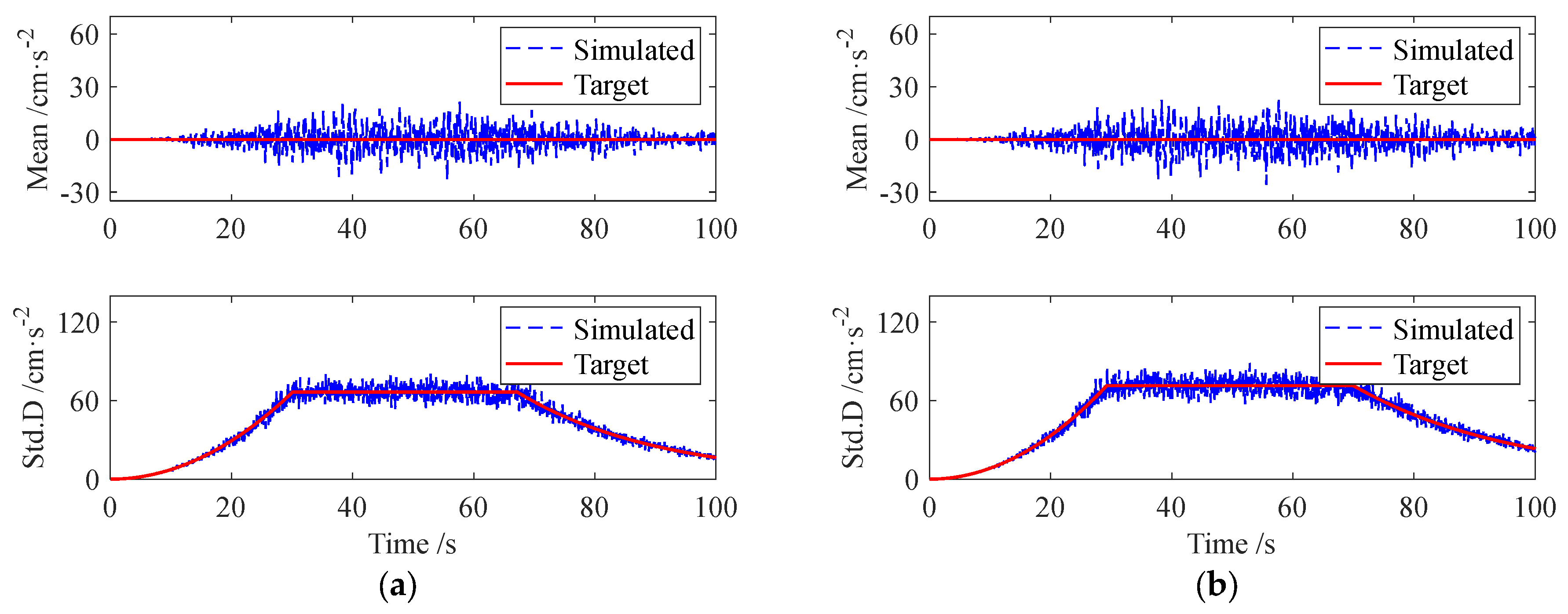
For the intensity-modulating function, the model suggested by Amin-Ang [23], which can reflect the non-stationary characteristics of ground motion, is employed in this paper and is given by the following:

$$q(t; {\mathsf{\lambda }}_{q_i}^u)=\left\{\begin{array}{cc}{t}^2/{(t_{1_1}^u)}^2& 0\le t\le t_{1_i}^u\\ 1& t_{1_i}^u\le t\le t_{2_i}^u\\ {\mathrm{e}}^{-{\alpha }_i^u\left(t-t_{2_i}^u\right)}& t_{2_i}^u\le t\end{array}\right.$$

(3)

where $t_{1_i}^u$ and $t_{2_i}^u$ indicate the arrival time and the end time of the stationary stage of the ground motion; ${\alpha }_i^u$ indicates the decay coefficient of the decay stage of the ground motion. In this context, the parameter vector of $q(t; {\mathsf{\lambda }}_{q_i}^u)$ can defined as ${\mathsf{\lambda }}_q=(t_{1_i}^u,t_{2_i}^u,{\alpha }_i^u)$. This model is acceptable for both high- and low-frequency components.

For the PSD of the corresponding stationary high-frequency component process, the Clough–Penzien model is employed in this paper [24]:

$$\overline{S}(\omega ;{\mathsf{\lambda }}_{{\overline{S}}_i}^u)=\frac{{({\omega }_{\mathrm{g},i}^u)}^4+4{({\xi }_{\mathrm{g},i}^u{\omega }_{\mathrm{g},i}^u\omega )}^2}{{[{\omega }^2-{({\omega }_{\mathrm{g},i}^u)}^2]}^2+4{({\xi }_{\mathrm{g},i}^u{\omega }_{\mathrm{g},i}^u\omega )}^2}·\frac{{\omega }^4}{{({\omega }^2-{({\omega }_{\mathrm{f},i}^u)}^2)}^2+4({\xi }_{\mathrm{f},i}^u{\omega }_{\mathrm{f},i}^u\omega )}{S}_{0,i}^u$$

(4)

To ensure the rationality of the seismic spectrum energy in this PSD function, parameters ${\omega }_{\mathrm{g},i}^u$ and ${\xi }_{\mathrm{g},i}^u$ are the filter parameters of the widely used Kanai–Tajimi spectrum, namely, the dominant frequency and the critical damping of the soil layer, respectively. ${\omega }_{\mathrm{f},i}^u$ and ${\xi }_{\mathrm{f},i}^u$ are the parameters of a second filter to ensure a finite power for ground displacement. $S_{0,i}^u$ is the spectral intensity factor, which indicates the intensity of the white noise bedrock acceleration process and can be expressed as follows [25]:

$$S_{0,i}^u={(\frac{A_i^u}{{\overline{r}}_i^u})}^2\frac{1}{E_i^u}; E_i^u=\frac{1}{S_{0,i}^u}{\displaystyle {\int }_{-\infty }^{\infty }\overline{S}(\omega ;{\mathsf{\lambda }}_{{\overline{S}}_i}^u)\mathrm{d}\omega }$$

(5)

where $A_i^u$ indicates the peak ground acceleration (PGA); ${\overline{r}}_i^u$ indicates the peak factor. In this context, the parameter vector of $\overline{S}(\omega ;{\mathsf{\lambda }}_{{\overline{S}}_i}^u)$ can be written as ${\mathsf{\lambda }}_{{\overline{S}}_1}=({\omega }_{\mathrm{g},i}^u,{\xi }_{\mathrm{g},i}^u,{\omega }_{\mathrm{f},i}^u,{\xi }_{\mathrm{f},i}^u,{\overline{r}}_i^u,A_i^u)$.

As mentioned in Equations (2)–(5), the EPSD parameter vectors of high- and low-frequency component processes can defined as follows:

$${\mathsf{\lambda }}_{{\overline{S}}_i}^u=({\mathsf{\lambda }}_{{\overline{S}}_1},{\mathsf{\lambda }}_q)=({\omega }_{\mathrm{g},i}^u,{\xi }_{\mathrm{g},i}^u,{\omega }_{\mathrm{f},i}^u,{\xi }_{\mathrm{f},i}^u,{\overline{r}}_i^u,A_i^u,t_{1_i}^u,t_{2_i}^u,{\alpha }_i^u)$$

(6)

It can be seen that the EPSD parameters can be divided into three parts: the PSD parameters control the spectrum characteristic; the intensity parameters control the amplitude characteristic; and the intensity-modulating function parameters control the duration characteristic.

3.2. The Identification of EPSD Parameter Vectors

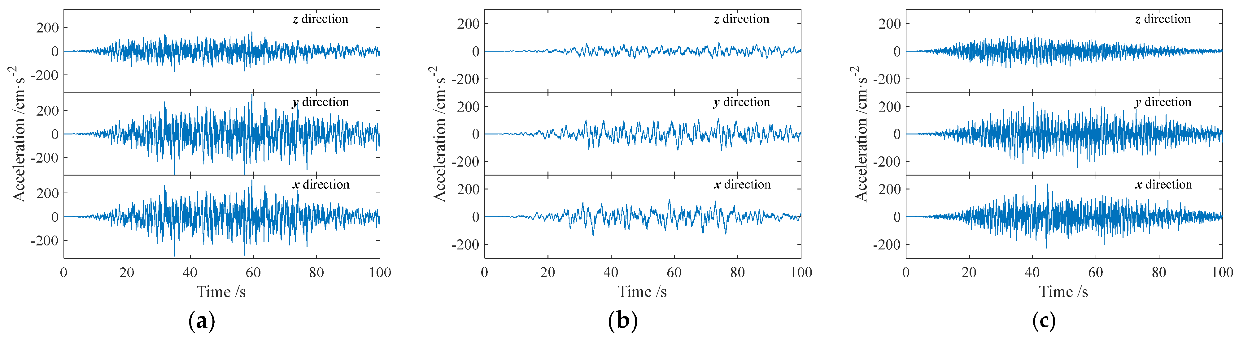
The EPSD parameters of high- and low-frequency component processes in different directions are associated with the soil conditions, which may be discerned and ascertained by analyzing the recorded data of multi-directional long-period ground motion at a specific site. To this end, the high- and low-frequency components of the u-th direction of any measured multi-directional long-period ground motion record can be defined as $a_i^u(t)$ and $i=1,2$; $u=1,2,3$ indicates the frequency components and directions of $a_i^u(t)$. What needs to be further explained is the fact that the measured record $a_i^u(t)$ is regarded as a stochastic process with one sample, and the corresponding estimated ESPD function of $a_i^u(t)$ is $S_i^u(\omega ,t)$.

In a broad sense, the total energy of $a_i^u(t)$ can be characterized using Arias’ intensity [26]. Additionally, Arias’ time-varying intensity provides insight into the temporal energy distribution in and non-stationarity of intensity, regardless of the specific soil conditions. The time-varying normalized energy distribution function (NEDF) of $a_i^u(t)$ can be mathematically represented as follows:

$$I_i^u(t)=\frac{{\displaystyle {\int }_0^t{[a_i^u(t)]}^2}\mathrm{d}t}{{\displaystyle {\int }_0^{T_{}^u}{[a_i^u(t)]}^2}\mathrm{d}t},$$

(7)

in which $T^k$ indicates the recorded duration of $a_i^u(t)$.

Moreover, the NEDF of $a_i^u(t)$ can be represented by means of the EPSD function, as utilized in this study, in accordance with Parseval’s theorem. This theorem states that the total energy of a signal in the time domain is equivalent to its total energy in the frequency domain. In this end, the NEDF of the stochastic process for which the corresponding EPSD function is $S(\omega ,t; {\mathsf{\lambda }}_{S_i}^u)$ can be defined as follows:

$$P(t;{\mathsf{\lambda }}_{S_i}^u)=\frac{{\displaystyle {\int }_0^t{\displaystyle {\int }_{-\infty }^{\infty }S(\omega ,t; {\mathsf{\lambda }}_{S_i}^u)}\mathrm{d}\omega \mathrm{d}t}}{{\displaystyle {\int }_0^{\infty }{\displaystyle {\int }_0^{\infty }S(\omega ,t; {\mathsf{\lambda }}_{S_i}^u)}\mathrm{d}\omega \mathrm{d}t}}=\frac{{\displaystyle {\int }_0^t{\left|q(t; {\mathsf{\lambda }}_{q_i}^u)\right|}^2\mathrm{d}t}}{{\displaystyle {\int }_0^{\infty }{\left|q(t; {\mathsf{\lambda }}_{q_i}^u)\right|}^2\mathrm{d}t}}=P(t; {\mathsf{\lambda }}_{q_i}^u)$$

(8)

It is evident that the NEDF solely pertains to the parameter vector of the intensity-modulating function. In this context, by taking $I_i^u(t)$ as the target, the parameter vector ${\mathsf{\lambda }}_{q_i}^u$ of $a_i^u(t)$ can be identified utilizing the best-square approximation principle:

$${\displaystyle {\int }_0^{T_{}^u}{\left|P(t;{\mathsf{\lambda }}_{S_i}^u)-I_i^u(t)\right|}^2}\mathrm{d}t\to \min$$

(9)

Furthermore, considering the substantial variation in recording duration and step length among different measured records, the average values of the identified parameters of the intensity modulation function are computed in this research to effectively capture the statistical properties of non-stationary multi-directional long-period ground motions under various soil conditions.

Moreover, concerning the energy characteristics of the ground motion, the total energy of $a_i^u(t)$ in the time domain is equal to that in the frequency domain according to Parseval’s theorem [27]:

$${(\frac{A_i^u}{{\overline{r}}_i^u})}^2{\displaystyle {\int }_0^{\infty }{\left|q(t; {\mathsf{\lambda }}_{q_i}^u)\right|}^2\mathrm{d}t}={\displaystyle {\int }_0^{\infty }{[a_i^u(t)]}^2}\mathrm{d}t$$

(10)

Actually, ${(\frac{A_i^u}{{\overline{r}}_i^u})}^2$ is the response variance of $a_i^u(t)$. In this context, the peak factor can be obtained using Equation (11) since the PGA of $a_i^u(t)$ can be easily extracted, as follows:

$${\overline{r}}_i^u=A_i^u\sqrt{\frac{t_{2_i}^u-\frac{4}{5}{t}_{1_i}^u+\frac{1-\exp [-2{\alpha }_i^u(T-t_{2_i}^u)]}{2{\alpha }_i^k}}{{\displaystyle {\int }_0^{\infty }{[a_i^u(t)]}^2}\mathrm{d}t}}$$

(11)

What needs further explaining is the fact that this research uses the average peak factor determined across various soil conditions as the recommended value, as the influence of the peak factor on ground motion amplitude is observed to be linear.

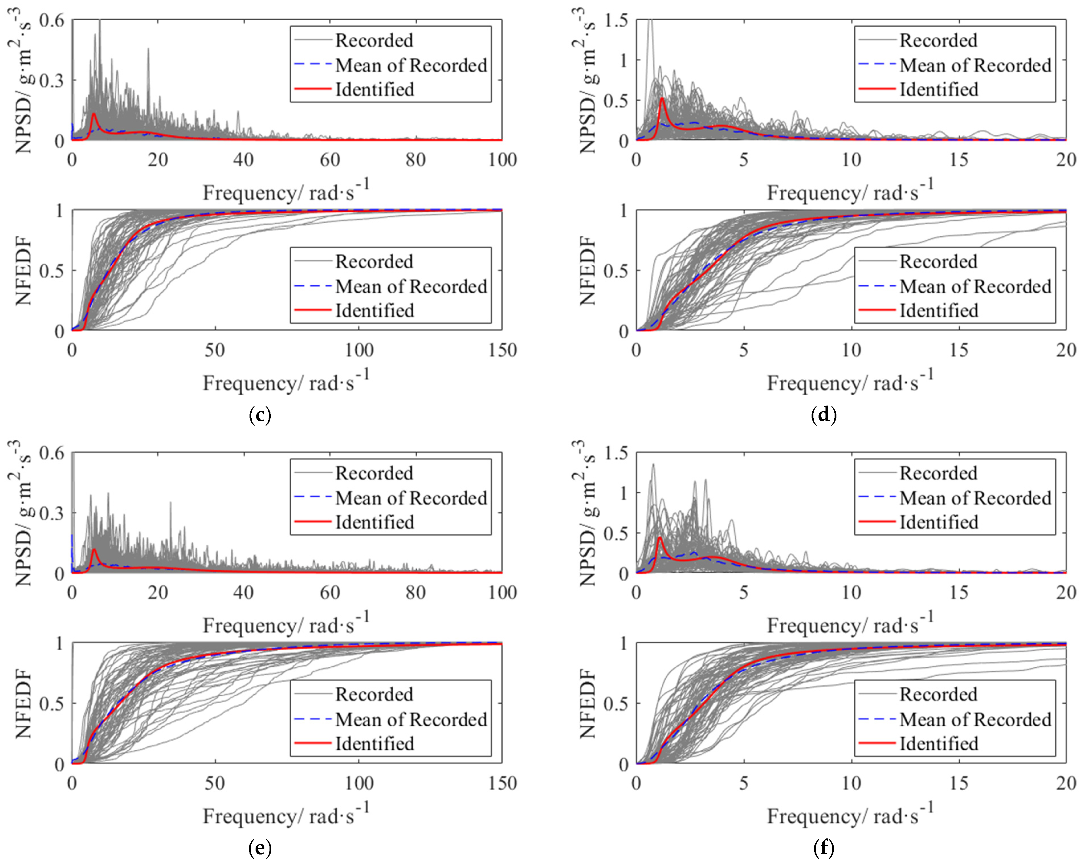
The remaining parameters that influence the shape of the spectrum can only be identified using the PSD function, as the identification of the parameters influencing duration and amplitude has been completed. Generally speaking, the PSD of $a_i^u(t)$ can be roughly estimated utilizing MATLAB’s toolbox function ‘pwelch’. Additionally, this work utilizes the normalized frequency domain energy distribution function (NFEDF) to mitigate the influence of the peak ground acceleration (PGA) and the peak factor on the spectral features. The NFEDF, denoted as ${\overline{F}}_i^u(\omega )$, is defined in the following manner:

$${\overline{F}}_i^u(\omega )=\frac{{\displaystyle {\int }_{-\infty }^{\omega }{F}_i^u(\omega )\mathrm{d}\omega }}{{\displaystyle {\int }_{-\infty }^{\infty }{F}_i^u(\omega )\mathrm{d}\omega }}$$

(12)

where $F_i^u(\omega )$ indicates the estimated PSD of $a_i^u(t)$. Furthermore, in order to accurately represent the energy distribution across the frequency domain for both high- and low-frequency components under varying soil conditions, this research uses the average of the estimated NFEDF, $H_i^u(\omega )$, of the corresponding measured records.

Correspondingly, the NFEDF can be modeled using the PSD model proposed in this paper, as follows:

$$\overline{H}(\omega ; {\mathsf{\lambda }}_{{\overline{S}}_i}^u )=\frac{{\displaystyle {\int }_{-\infty }^{\omega }\overline{S}(\omega ; {\mathsf{\lambda }}_{{\overline{S}}_i}^u)\mathrm{d}\omega }}{{\displaystyle {\int }_{-\infty }^{\infty }\overline{S}(\omega ; {\mathsf{\lambda }}_{{\overline{S}}_i}^u)\mathrm{d}\omega }}$$

(13)

Taking $H_i^u(\omega )$ as the target, the parameter vector of the PSD functions can be identified utilizing the best-square approximation principle:

$${\displaystyle {\int }_{-\infty }^{\infty }{\left|\overline{H}(\omega ; {\mathsf{\lambda }}_{{\overline{S}}_i}^u )-H_i^u(\omega )\right|}^2}\mathrm{d}\omega \to \min$$

(14)

In this manner, the orderly identification of the EPSD parameter vector ${\mathsf{\lambda }}_{{\overline{S}}_i}^u$ is completed, namely, from the duration to the energy and then to the spectrum.

In summary, the process of identification can be condensed into the following steps:

(a)

Employing NEDF to ascertain the parameters of the intensity modulation function for each recorded measurement under varying soil conditions and, subsequently, averaging these parameters to obtain the recommended values for the high- and low-frequency component processes.

(b)

The utilization of response variance for the purpose of identifying the peak factor is suggested subsequent to the acquisition of parameters governing the duration characteristics. The average value of the detected peak factor is then considered as the recommended parameters for high- and low-frequency component processes.

(c)

This study employs the averaged NFEDF across various soil conditions to determine the optimal parameters for the high- and low-frequency component processes of each direction that influence the spectral features.

Further elucidation is warranted on the execution of the identification work, which is conducted in accordance with the prevailing soil conditions.

Figure 3 and Figure 4 illustrate the identified results of the EPSD parameters for site 2 pertaining to both high- and low-frequency components in each direction. The results clearly indicate that the identified value can be considered as the “mean” in terms of the optimal square approximation of the recorded value. These findings provide strong evidence for the efficacy of the parameter identification approach proposed in this study.

Table 3. The recommended EPSD parameters of long-period ground motions.

Site Classes	Frequency Components	Direction	Parameters
			${\mathit{t}}_{\mathbf{1}} \mathbf{(}\mathbf{s}\mathbf{)}$	${\mathit{t}}_{\mathbf{2}} \mathbf{(}\mathbf{s}\mathbf{)}$$+{\mathit{t}}_{\mathbf{1}} \mathbf{(}\mathbf{s}\mathbf{)}$	$\mathsf{\alpha }$	${\mathsf{\omega }}_{\mathbf{g}} \mathbf{(}\mathbf{rad}\mathbf{/}\mathbf{s}\mathbf{)}$	${\mathsf{\xi }}_{\mathbf{g}}$	${\mathsf{\omega }}_{\mathbf{f}} \mathbf{(}\mathbf{rad}\mathbf{/}\mathbf{s}\mathbf{)}$	${\mathsf{\xi }}_{\mathbf{f}}$
1	High	x	27.54	60.98	0.10	19.67	0.37	5.71	0.15
		y	28.72	68.61	0.09	19.01	0.38	5.45	0.16
		z	21.61	62.69	0.08	21.84	0.51	5.46	0.16
	Low	x	27.43	64.04	0.06	4.38	0.34	1.06	0.12
		y	29.58	70.67	0.05	4.33	0.34	1.06	0.14
		z	30.04	77.26	0.06	4.18	0.34	1.13	0.12
2	High	x	30.12	67.16	0.04	17.72	0.37	4.88	0.18
		y	29.26	69.97	0.04	18.45	0.37	4.96	0.16
		z	20.25	59.45	0.05	22.66	0.48	5.04	0.16
	Low	x	32.73	73.97	0.04	4.23	0.35	1.11	0.15
		y	33.47	82.68	0.03	4.44	0.35	1.17	0.16
		z	33.61	89.01	0.03	4.04	0.36	1.05	0.19
3	High	x	23.22	62.59	0.07	18.07	0.38	5.41	0.17
		y	22.74	58.41	0.06	17.45	0.36	4.49	0.18
		z	19.26	58.43	0.05	29.11	0.54	5.79	0.18
	Low	x	29.30	83.07	0.05	4.30	0.34	1.29	0.14
		y	25.28	73.77	0.04	4.47	0.34	1.30	0.14
		z	34.51	95.26	0.04	4.18	0.37	1.39	0.14

presents the EPSD parameters that are recommended for multi-directional long-period ground motions. On the other hand,

Table 4. Average ratio of the amplitude parameter between the high- and low-frequency components in the x direction.

Site Classes	Parameters
	${\mathit{A}}_{{}_{\mathbf{1}}}\mathbf{/}{\mathit{A}}_{{}_{\mathbf{2}}}$	${\overline{\mathit{r}}}_{\mathbf{1}}\mathbf{/}{\overline{\mathit{r}}}_{\mathbf{2}}$
1	1.2242	1.1888
2	1.9203	1.2727
3	1.3303	1.0816

and

Table 5. Average ratio of the amplitude parameter of the high- and low-frequency components between different directions.

Parameters	Site Classes	Frequency Components	Directions
			x/y	x/z
A	1	1	1.03	1.76
		2	0.99	1.63
	2	1	0.99	1.93
		2	0.94	1.81
	3	1	0.97	1.66
		2	1.01	2.10
r	1	1	0.96	0.91
		2	0.99	1.01
	2	1	1.00	0.89
		2	1.00	1.04
	3		0.98	0.93
			0.98	1.06

display the amplitude parameter ratios associated with various frequency components, direction components, and soil conditions. These tables provide valuable insights regarding direction, frequency components, and site characteristics.

(1)

The engineering features of the x- and y-direction components of multi-dimensional ground motion are similar. However, the z-direction component exhibits a longer duration, a greater dominant frequency, and a lower energy in comparison to the horizontal components.

(2)

In contrast to the high-frequency components, the low-frequency components exhibit higher energy levels and are mostly focused within the low-frequency range. Moreover, it is worth noting that the length of the low-frequency components is comparatively longer when compared to that of the high-frequency components.

(3)

As the soil conditions undergo softening, the duration of the ground motion progressively elongates; the dominant frequency gradually diminishes, and the critical damping increases roughly. Moreover, it is evident that, as the soil conditions transition to a softer state, there is a gradual drop in the average ratio of PGA. Specifically, soft soil exhibits a greater ability to magnify the PGA of low-frequency components compared to hard soil.

Apparently, the recommended values are identified from the selected long-period ground motions from databases of each soil condition and reflect the statistical characteristics of the spectrum energy and time-varying-intensity of long-period ground motions. Because of this, the recommended values can generally be used.

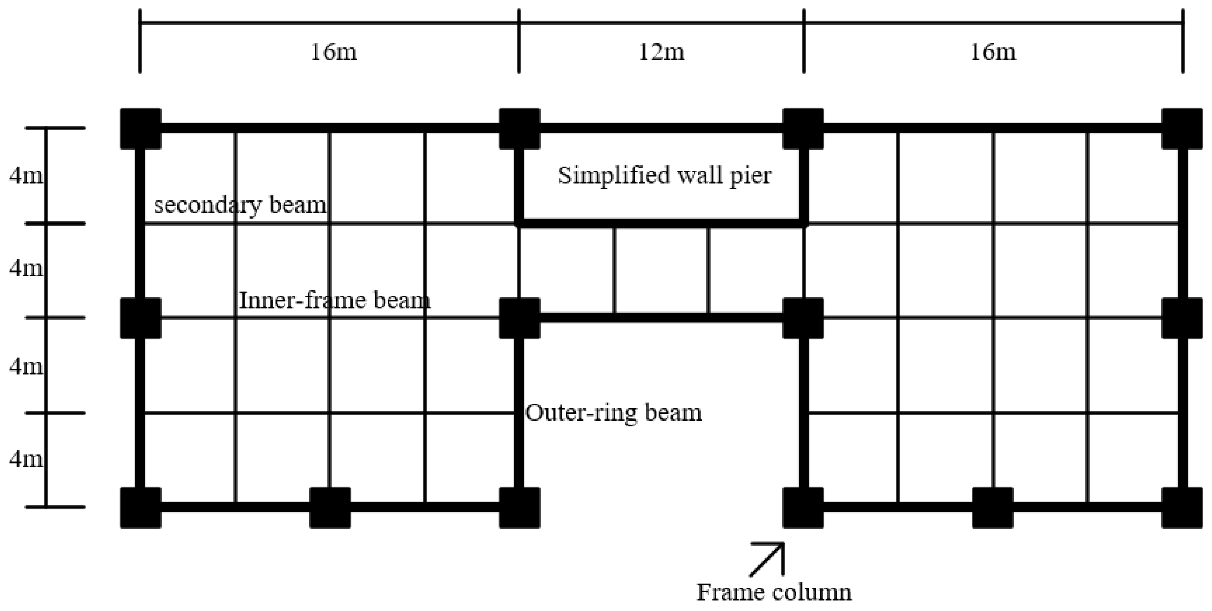
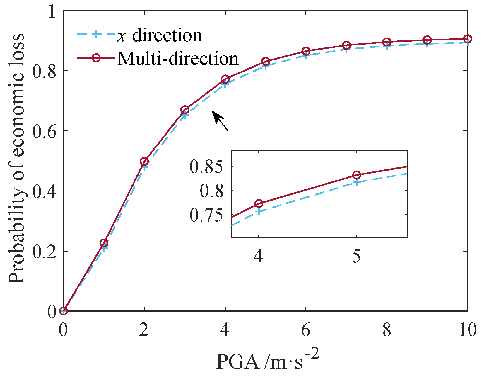
In a further study, more refined FEM models of high-rise structures will be introduced to investigate the real dynamic response and loss probability of high-rise structures.

4. POD Representation of a Multi-directional Long-Period Ground Motion Vector Process

4.1. The Basic Theory of the POD Method

In this study, the multi-directional long-period ground motion process $Y_{}^u(t) (u=1,2,3)$ is regarded as the sum of high- and low-frequency component processes, i.e., $X_i^u(t) (i=1,2)$. $X_i^u(t)$, with three directions, can be regarded as one dimensional three-variable (1D-2V) multivariate non-stationary stochastic processes: namely, ${\mathit{X}}_i(t)=[X_i^1(t),X_i^2(t),X_i^3(t)]$, $\mathit{Y}(t)=[Y_{}^1(t),Y_{}^2(t),Y_{}^3(t)]$, and $\mathit{Y}(t)={\mathit{X}}_1(t)+{\mathit{X}}_2(t)$. In this context, the multi-directional long-period ground motion process can be obtained through the superimposition of simulated multi-directional high- and low-frequency component processes. Generally, the two-sided EPSD matrix of ${\mathit{X}}_i(t)$ can be expressed as follows [28]:

$${\mathit{S}}_{X_i}(\omega ,t)=\left[\begin{array}{ccc}S(\omega ,t; {\mathsf{\lambda }}_{S_i}^1)& S(\omega ,t; {\mathsf{\lambda }}_{S_i}^{12})& S(\omega ,t; {\mathsf{\lambda }}_{S_i}^{13})\\ S(\omega ,t; {\mathsf{\lambda }}_{S_i}^{21})& S(\omega ,t; {\mathsf{\lambda }}_{S_i}^2)& S(\omega ,t; {\mathsf{\lambda }}_{S_i}^{23})\\ S(\omega ,t; {\mathsf{\lambda }}_{S_i}^{31})& S(\omega ,t; {\mathsf{\lambda }}_{S_i}^{32})& S(\omega ,t; {\mathsf{\lambda }}_{S_i}^3)\end{array}\right]$$

(15)

where $S(\omega ,t; {\mathsf{\lambda }}_{S_i}^{uv}) (u,v=1,2,3)$ indicates the CPSD of the u-th-direction and v-th-direction components of high- or low-frequency component processes and can be defined as follows:

$$S(\omega ,t; {\mathsf{\lambda }}_{S_i}^{uv}) =\gamma \left(\omega \right)\sqrt{S(\omega ,t; {\mathsf{\lambda }}_{S_i}^u)·S(\omega ,t; {\mathsf{\lambda }}_{S_i}^v) }$$

(16)

Here, $\gamma \left(\omega \right)$ indicates the coherence function for multi-directional ground motions.

Further, the EPSD matrix, ${\mathit{S}}_{X_i}(\omega ,t)$, can be decomposed as follows:

$${\mathit{S}}_{X_i}(\omega ,t)=\mathit{D}(\omega ,t)\mathsf{\gamma }\left(\omega \right){\mathit{D}}^{\mathrm{T}\ast }(\omega ,t)$$

(17)

where superscript T and * indicate the matrix transpose and conjugate, respectively. $\mathit{D}(\omega ,t)=diag[\sqrt{S(\omega ,t; {\mathsf{\lambda }}_{S_i}^1)}$$,\sqrt{S(\omega ,t; {\mathsf{\lambda }}_{S_i}^2)},\sqrt{S(\omega ,t; {\mathsf{\lambda }}_{S_i}^3)}]$ indicates the EPSD diagonal matrix, and the coherence function for multi-directional ground motions, $\gamma \left(\omega \right)$, proposed by Matsushima Toyo can be defined as follows:

$$\mathsf{\gamma }(\omega )=\left[\begin{array}{ccc}1& 1& 0.6\\ 1& 1& 0.6\\ 0.6& 0.6& 1\end{array}\right]$$

(18)

Evidently, $\mathsf{\gamma }(\omega )$ is a non-negative Hermitian matrix; thus, it can be decomposed utilizing eigen decomposition into the following form:

$$\left\{\begin{array}{l}\mathsf{\gamma }(\omega )=\mathsf{\Psi }(\omega )\mathsf{\Lambda }(\omega ){\mathsf{\Psi }}^{\ast \mathrm{T}}(\omega )\hfill \\ {\mathsf{\Psi }}^{\ast \mathrm{T}}(\omega )\mathsf{\Psi }(\omega )=\mathbf{I}\hfill \end{array}\right.$$

(19)

where $\mathsf{\Psi }(\omega )=[{\mathsf{\psi }}_1(\omega ),{\mathsf{\psi }}_2(\omega ),{\mathsf{\psi }}_3(\omega )]$ is the eigenvectors’ matrix, in which element ${\mathsf{\psi }}_r(\omega )={[{\varphi }_{1r}(\omega ),{\varphi }_{2r}(\omega ),{\varphi }_{3r}(\omega )]}^{\mathrm{T}}$, and represents the shape of the r-th $(r=1,3)$ eigenmode. $\mathsf{\Lambda }(\omega )=\mathrm{diag}[{\mathsf{\Lambda }}_1(\omega ),{\mathsf{\Lambda }}_2(\omega ),{\mathsf{\Lambda }}_3(\omega )]$ indicates the diagonal eigenvalues’ matrix, in which element ${\mathsf{\Lambda }}_r$ represents the energy of the r-th eigenmode; I indicates the identity matrix of size $3\times 3$. In this context, ${\mathsf{\psi }}_r(\omega )$ can be further expressed in the following form:

$${\mathsf{\psi }}_r(\omega )={\mathsf{\chi }}_r({\omega }_k)+\mathrm{i}{\mathcal{Z}}_r({\omega }_k)$$

(20)

where i indicates the imaginary unit.

Suppose that ${\mathit{X}}_i(t)=[X_i^1(t),X_i^2(t),X_i^3(t)]$ is a real-valued, zero-mean, 1D-3V non-stationary stochastic process, and the multi-directional long-period ground motion process $\mathit{Y}(t)$ with a u-th direction can be written as follows: [29,30]

$$\begin{array}{l}{Y}^u(t)={\displaystyle \sum _{i=1}^2{X}_i^u(t)}\approx 2{\displaystyle \sum _{i=1}^2{\displaystyle \sum _{r=1}^3{\displaystyle \sum _{k=1}^N\sqrt{S(\omega ,t; {\mathsf{\lambda }}_{S_i}^u){\mathsf{\Lambda }}_r({\omega }_k)\Delta \omega }}}\times \left[{\chi }_{ur}({\omega }_k)\right.\left(R_{rk}\cos {\omega }_{k}t-\right.\left.Q_{rk}\sin {\omega }_{k}t\right)}\\ \hspace{1em}\hspace{1em}\hspace{1em} -{\mathcal{Z}}_{ur}({\omega }_k)\left.\left(R_{rk}\sin {\omega }_{k}t+Q_{rk}\cos {\omega }_{k}t\right)\right]\end{array}$$

(21)

where ${\omega }_k$ indicates the discrete sample frequency series; $\Delta \omega ={\omega }_{\mathrm{u}}/N$ indicates the frequency increment, and N indicates the number of frequency intervals; $\{R_{rk},Q_{rk}\}$ refers to a set of zero-mean standard orthogonal stochastic variables that satisfy the following basic conditions:

$$\begin{array}{l}E\left[R_{rk}\right]=E\left[Q_{rk}\right]=0, E\left[R_{rk}{Q}_{ls}\right]=0,\\ E\left[R_{rk}{R}_{ls}\right]=E\left[Q_{rk}{Q}_{ls}\right]={\displaystyle \frac{1}{2}}{\delta }_{rl}{\delta }_{ks},\\ r,l=1,..,M, k,s=1,2,\cdots ,N\end{array}$$

(22)

Generally, the random variables set can be defined using a set of random phase angles, as follows:

$$\left\{\begin{array}{c}{R}_{rk}=\cos {\alpha }_{rk}\\ I_{rk}=\sin {\alpha }_{rk}\end{array}\right.$$

(23)

where ${\alpha }_{rk}$ indicates a set of random phase angles, uniform in the interval $(0, 2\mathsf{\pi })$. Of course, Equation (23) completely satisfies the basic conditions defined in Equation (22).

4.2. Representative Sample Realization Procedures for a Multi-Directional Long-Period Ground Motion Process

The implementation of representative sample realization for the multi-directional long-period ground motion process can be achieved through the following procedures:

(1)

The PGA and peak ratio of the low-frequency components in the x direction can be obtained using Table 4, if the PGA and peak ratio of the high-frequency components in the x direction have been provided.

(2)

The PGA and peak ratio of the high- and low-frequency components for three directions can be further acquired using Table 5, followed by step 1.

(3)

In this study, we aim to develop EPSD functions for both low- and high-frequency component processes in three different directions. The parameters of PGA and peak ratio are considered in the first two steps, while the other parameters can be found in Table 3.

(4)

The high- and low-frequency components in the three directions are generated using the POD approach. By superimposing the simulated high- and low-frequency components, multi-directional long-period ground motion can be achieved.

5. Numerical Example

In this numerical example, the EPSD parameters of the low- and high-frequency component processes in three directions refer to Table 3. Moreover, the PGA and peak factor of the high-frequency component in the x direction are taken to be $200 \mathrm{cm}/{\mathrm{s}}^2$ and 3, and the corresponding ones for the high-frequency components in the other directions and the low-frequency components in all three directions can be obtained from Table 4 and Table 5 (for the specific steps, refer to Section 4.2). Furthermore, the simulation parameters for the POD approach, which are shared by both the low- and high-frequency component processes, are listed in

Table 6. The parameters for the simulation parameters for the POD-DR formula.

Parameter	Value
Upper cutoff frequency (rad/s)	${\omega }_{\mathrm{u}}=240$
Frequency step (rad/s)	$\Delta \omega =0.15$
Total number of frequencies	$N=1600$
Simulated duration (s)	$T=100$
Time-step (s)	$\Delta t=0.02$
Total number of times	$N_t=5000$
Number of samples	$n_{\mathrm{sel}}=144$

.

Figure 5 illustrates representative samples of simulated multi-directional long-period ground motion processes using the POD method. It also shows the corresponding high- and low-frequency component processes in three directions. It is evident that the superimposed representative samples exhibit distinct characteristics of multi-directional long-period ground motions. Specifically, the simulated ground motions are non-stationary in the frequency domain and possess prominent long-period components. Moreover, it can be seen that the horizontal components have similar features, while the vertical components have a longer duration, a greater dominant frequency, and a lower energy than the horizontal components. Further, it can be seen that the mean and standard deviation of the simulated samples in the x direction correspond well to the respective corresponding target values in Figure 6, which verify the correctness of the simulation results in this paper.

In order to demonstrate the efficacy and practicality of EPSD functions and their parameters as proposed in this study, Figure 7 presents a comparison of the average seismic influence coefficient between the simulated representative samples and the measured records of site 2. This comparison is conducted for three scenarios: low-frequency component process, high-frequency component process, and superimposed multi-directional long-period ground motion process. Additionally, it is important to acknowledge that the PGA values obtained from the measured records and the simulated representative samples are scaled to $200 \mathrm{cm}/{\mathrm{s}}^2$. The observed data indicate a close correspondence between the average seismic influence coefficient of the samples and the one derived from the measured records. Specifically, the optimal level of consistency is kept in close proximity to the primary peak of the average seismic effect coefficient. The successful establishment of a consistent relationship between the statistical properties of stochastic simulated multi-directional long-period ground motions and the corresponding observed records has enhanced the comprehensiveness of applying the stochastic simulation approach in engineering practice.

6. The Economic Assessment of a High-Rise Frame Structure under Multi-directional Long-Period Ground Motion

This paper involves the inclusion of a typical high-rise frame structure to showcase the technical application of the suggested model. The investigation focuses on the assessment of seismic economic loss under synthetic ground motion induced by the aforementioned stochastic model.

6.1. Seismic Vulnerability Theory Based on the IDA Method

The incremental dynamic analysis (IDA) method is an analytical technique that uses dynamic time history analysis to evaluate the changes in the sustained response of a structure by manipulating the intensity of seismic motion input. This study aims to develop a quantitative correlation between the responses of structures and seismic intensity, thereby illuminating the relationship between variations in structural performance. Furthermore, it thoroughly considers the seismic requirements and structural capabilities of a building. In general, the technique of IDA can be summarized as follows [31,32,33]:

(1)

Determine the seismic intensity index IM, which is usually taken as the PGA or the acceleration response spectrum with a damping ratio of $\xi$. For the high-rise frame structure employed in this paper, PGA is taken as the seismic intensity index IM.

(2)

Determine the structural damage index DM. The maximum story–drift ratio ${\theta }_{\max }$, which can better reflect the damage situation and performance state of structural components, is taken as the structural damage index DM in this study.

(3)

Adjusting the seismic intensity of input excitation in equal steps, i.e., 0.1 g, 0.2 g, 0.3 g, …, 1 g.

(4)

Input the simulated multi-directional long-period ground motions with different intensity into the high-rise frame structure to obtain the corresponding maximum story–drift ratio.

Actually, it can be acknowledged through the IDA method that there is an exponential correlation between the structural damage index DM and the seismic intensity index IM, and it can be described as follows:

$$DM=a·I{M}^b$$

(24)

Meanwhile, Equation (24) can be further expressed by logarithmizing both of its sides:

$$\ln DM=\ln (a)+b·\ln (IM)=A+B\ln IM$$

(25)

where A and B are constants.

If we assume that the seismic resistance ability of a structure at a certain level of performance is defined as C and that the structural response capacity of a structure under a certain seismic intensity is D, the structural failure probability can be written as follows:

$$P_{\mathrm{f}}=P(R\le 0)=P(C/D\le 1)$$

(26)

Suppose that C and D correspond to a normal distribution, as follows:

$$C~N({\mu }_C,{\sigma }_C)$$

(27)

$$D~N({\mu }_D,{\sigma }_D)$$

(28)

where ${\mu }_C$ and ${\sigma }_C$, respectively, denote the mean and standard deviation of the seismic resistance ability, and ${\mu }_D$ and ${\sigma }_D$, respectively, denote the mean and standard deviation of the structural response capacity. This way, $R$ also corresponds to a normal distribution, and its mean and standard deviation are $\mu ={\mu }_C-{\mu }_D$ and $\sigma =\sqrt{{\sigma }_C^2+{\sigma }_D^2}$. Further, convert R to a standard normal distribution, as follows:

$$P_{\mathrm{f}}=P(R\le 0)=P(T\le \frac{\mu }{\sigma })=\Phi (\frac{-\ln ({\mu }_C/{\mu }_D)}{\sqrt{{\beta }_C^2+{\beta }_D^2}})$$

(29)

where ${\beta }_C$ and ${\beta }_D$, respectively, denote a logarithmic standard deviation. Actually, ${\mu }_D$ can be replaced with DM, and $\sqrt{{\beta }_C^2+{\beta }_D^2}=0.5$, as the seismic intensity index IM is PGA. Combining Equations (24) and (29), the calculation formula for the failure probability can be written as in Ref. [34]:

$$P_{\mathrm{f}}=\Phi (\frac{\ln (\exp (A)·I{M}^B/{\mu }_D)}{0.5})$$

(30)

6.2. Engineering Background and Vulnerability Analysis

In order to investigate the seismic economic loss of a nonlinear frame structure subjected to multi-directional long-period ground motions, an 18-story high-rise frame structure with a floor height of 3 m is studied herein as the engineering object. Figure 8 shows the structural plan, and the sizes of the structural members are listed in

Table 7. The section size of the structural members.

Structural Members	Section Size (m)	Concrete	Elastic Modulus (Pa)
Frame column	$1.1\times 1.1$	C40	$3.5\times {10}^{10}$
Outer-ring beam	$0.4\times 0.6$	C40	$3.5\times {10}^{10}$
Inner-frame beam	$0.5\times 0.8$	C40	$3.5\times {10}^{10}$
Secondary beam	$0.3\times 0.5$	C40	$3.5\times {10}^{10}$
Simplified wall pier	0.3	C40	$3.5\times {10}^{10}$
Roof panel	0.2	C30	$3.2\times {10}^{10}$
Peripheral wall	0.2	C30	$3.2\times {10}^{10}$

. For the convenience of calculation, the density of the reinforced concrete C30 and C40 is uniformly 2500 kg/m³; the elastic modulus is taken to be the elastic modulus of concrete, and Poisson’s ratio is taken to be 0.2. The finite element model shown in Figure 9 is established using the ANSYS software 19.0, and the columns and beams of the wall structure use the BEAM188 unit, and the floor and the exterior wall use the SHELL63 unit. Moreover, the results of the analysis of the first six vibration modes are listed in

Table 8. The results of the vibration mode analysis.

Order	1	2	3	4	5	6
Natural frequency (Hz)	1.70	2.75	3.36	5.83	7.01	7.15

, and it clearly acknowledges that the first order-of-vibration mode is just 1.70 Hz, which indicates that the model is a flexible structure and leans forward to resonate with low-frequency loads such as long-period ground motion. What needs to be further explained is the fact that, for the convenience of calculation in this paper, the elastic modulus taken is based on the elastic modulus of concrete, which may lead to a low natural period.

The external excitation of the multi-directional long-period ground motion, which can reflect the average seismic characteristics of site 2, is involved in this numerical example, and the comparison of the acceleration response spectrum between the simulated samples and the measured records is displayed in Figure 10, which demonstrates that the simulated samples have seismic engineering characteristics consistent with the measured records. Moreover, the number of simulated samples is 10, and the PGA of the x-directional long-period ground motion is 200 cm/s².

Figure 11a shows the story–drift ratio under a typical multi-directional long-period ground motion and a representative sample of x-directional long-period ground motion with an intensity of 1.0 g acting on the tenth story, and Figure 11b shows the maximum drift value as it changes by story. It can be seen from Figure 11a,b that the dynamic response of the aforementioned high-rise frame structure under the multi-directional long-period ground motion is more intense than that of the structure under the x-directional long-period ground motion.

Further, the quantitative indicator limits for different ultimate failure states of the structural response should be determined to evaluate the ultimate failure state of the structure. Based on the Code for the Seismic Design of Buildings (GB 50011-2010) [19], the failure state of the nonlinear frame structure can be divided into the following levels: basically intact, slightly damaged, moderately damaged, severely damaged, and collapsed; their corresponding descriptions are shown in

Table 9. The descriptions and quantitative indicators of each degree of structural damage [19].

Degree of Structural Damage	Descriptions	Quantitative Indicators (Inter-Story Drifts)
Basically intact	The main load-bearing components are intact, and very few load-bearing components are damaged, requiring no repair.	<1/500
Slightly damaged	Some load-bearing components have slight cracks, or some non-load-bearing components are damaged and do not require repair or minor repairs.	1/500
Moderately damaged	Most load-bearing components are slightly damaged, while some non-load-bearing components are severely damaged and require repair.	1/200
Severely damaged	Most load-bearing components have undergone severe damage or even collapsed.	1/100
Collapsed	Most of the main load-bearing components collapsed.	1/50

.

As mentioned previously, the exceeding probability of a nonlinear frame structure under different degrees of structural damage is shown in Figure 12. In this figure, it can be clearly seen that the failure probability of the structure under multi-directional ground motions is increased by around 1% compared to than that of the structure under the x-directional long-period ground motion. Moreover, according to the vulnerability curves of each degree of structural damage, the seismic fortification objectives of “not damaging during small earthquakes and not collapsing during large earthquakes” proposed in the Chinese seismic code can be met under structural earthquake action. Under rare earthquake action, namely, 0.2 g m/s², the probabilities of minor damage, moderate damage, severe damage, and collapse are 0.99, 0.98, 0.79, and 0.28, respectively.

6.3. Seismic Economic Loss Assessment

Generally, the seismic economic loss rate of a structure can be expressed as economic losses and replacement values, defined as follows:

$$DF=\frac{L}{R}$$

(31)

where DF denotes the damage factor, and L and R, respectively, indicate the economic losses and the replacement values. Moreover, the degree of structural damage and the economic loss rate have a certain relationship, which is described in

Table 10. The relationship between the degree of structural damage and the range of loss rate [35].

Degree of Structural Damage	Range of Economic Loss Rate (%)	Median Value of Economic Loss Rate
Basically intact	0	0
Slightly damaged	1~10	5
Moderately damaged	10~40	25
Severely damaged	40~80	60
Collapsed	80~100	90

.

According to Table 8 and the results of our vulnerability analysis, the loss rate can be represented with a vulnerability curve, as follows [35]:

$$\begin{array}{c}DF=0\times (1-P_1)+0.05\times (1-P_1-P_2)+0.25\times (1-P_1-P_2-P_3)+\\ 0.6\times (1-P_1-P_2-P_3-P_4)+0.9\times P_4\end{array}$$

(32)

where $P_1,P_2,P_3,P_4,P_5$, respectively, indicate exceeding probability. The economic loss rate can be further written as follows:

$$\begin{array}{c}L=DF\times R=R\times [0\times (1-P_1)+0.05\times (1-P_1-P_2)+0.25\times (1-P_1-P_2-P_3)+\\ 0.6\times (1-P_1-P_2-P_3-P_4)+0.9\times P_4]\end{array}$$

(33)

Following this, the probabilities of economic loss of a high-rise frame structure under multi-directional long-period ground motion and x-directional long-period ground motion, respectively, are displayed in Figure 13, which shows that the probability of economic loss of a frame structure under multi-directional long-period ground motion is around 1% higher than that of a structure under x-directional long-period ground motion, on average.

7. Conclusions

Utilizing measurable records, this study presents a stochastic model for high- and low-frequency component processes in three directions of long-period ground motions and achieves the aim of simulating the superposition of multi-directional long-period ground motion. Furthermore, an evaluation of the probability of failure and economic loss of a high-rise frame structure is performed under the action of simulated long-period ground motion in multiple directions. The detailed analysis and conclusion are as follows:

(1)

Long-period ground motion is characterized by significant frequency non-stationarity, which presents difficulties for traditional simulation techniques. Because of this, this investigation employs the EMD methodology to partition long-period ground motion into a superimposed form comprising components at high and low frequencies, and the seismic characteristics of these components are subsequently further investigated.

(2)

The EPSD functions are proposed in light of the aforementioned findings, and the corresponding EPSD parameters for three dimensions of high- and low-frequency components of long-period ground motions are identified utilizing the normalized energy distribution function and the normalized frequency domain energy distribution function.

(3)

Moreover, by integrating the coherence model of multi-directional ground motion and that of the high- and low-frequency components of long-period ground motions, the EPSD matrix for high- and low-frequency component processes in three directions is generated. Subsequently, the POD method can be employed to accomplish the superimposed simulation of a multi-directional long-period ground motion process. Furthermore, a numerical example is employed to validate the engineering applicability and accuracy of the proposed EPSD parameters for multi-directional long-period ground motion through a comparison with measured recordings.

(4)

The economic losses and failure probability of a high-rise frame structure subjected to simulated multi-directional long-period ground motion are investigated in this study, which found that long-period ground motion in multiple directions may result in a greater probability of economic losses than long-period ground motion in a single direction.

References

1. Koketsu, K.; Miyake, H. A seismological overview of long-period ground motion. J. Seismol. 2008, 12, 133–143. [Google Scholar] [CrossRef]
2. Yang, D.X.; Wang, W. Nonlocal period parameters of frequency content characterization for near-fault ground motions. Earthq. Eng. Struct. D 2012, 41, 1793–1811. [Google Scholar] [CrossRef]
3. Maeda, T.; Sasatani, T. Long-period ground motions from the 2003 Tokachi-oki earthquake. J. Seismol. 2008, 12, 243–253. [Google Scholar] [CrossRef]
4. Oana, A.; Kitamura, H.; Yoshie, K.; Sato, T. Qualitative evaluation of f-values of long-period ground motions for design earthquake motions. J. Struct. Constr. Eng. 2012, 77, 575–584. [Google Scholar] [CrossRef]
5. Chen, Q.J.; Li, Y.C. Simulation of Harmonic-like Long-period Ground Motion Based on Evolutionary Spectra and Orthogonal HHT Method. J. Hunan Univ. (Nat. Sci.) 2012, 39, 20–27. (In Chinese) [Google Scholar]
6. Dai, M.H. Quantitative Identification and Simulation of Multi-direction Long-Period Ground Motions. Ph.D. Thesis, Chongqing University, Chongqing, China, 2020. (In Chinese). [Google Scholar]
7. Chung, Y.L.; Nagae, T.; Matsumiya, T.; Nakashima, M. Seismic resistance capacity of beam–column connections in high-rise buildings: E-Defense shaking table test. Earthq. Eng. Struct. D 2011, 40, 605–622. [Google Scholar] [CrossRef]
8. Chung, Y.L.; Nagae, T.; Matsumiya, T.; Nakashima, M. Seismic capacity of retrofitted beam–column connections in high-rise steel frames when subjected to long-period ground motions. Earthq. Eng. Struct. D 2012, 41, 735–753. [Google Scholar] [CrossRef]
9. Chung, Y.L.; Nagae, T.; Hitaka, T.; Nakashima, M. Seismic resistance capacity of high-rise buildings subjected to long-period ground motions: E-Defense shaking table test. J. Struct. Eng. 2010, 136, 637–644. [Google Scholar] [CrossRef]
10. Takewaki, I.; Murakami, S.; Fujita, K.; Yoshitomi, S.; Tsuji, M. The 2011 off the Pacific coast of Tohoku earthquake and response of high-rise buildings under long-period ground motions. Soil Dyn. Earthq. Eng. 2011, 31, 1511–1528. [Google Scholar] [CrossRef]
11. Nagano, M.; Hida, T. Dynamic response characteristics of super high-rise residential buildings in Kanto and Kansai area during the great east Japan earthquake. In Proceedings of the International Symposium on Engineering Lessons Learned from the 2011 Great East Japan Earthquake, Tokyo, Japan, 1–4 March 2012. [Google Scholar]
12. Bai, Y.; Egashira, S.; Fujii, M.; Odawara, K.; Kawano, A.; Matsuo, S. 22722 Time History Analysis of High-Rise Buildings Considering The Strength Degradation: Part2. Time History Analysis of Past Generic High-Rise Steel MRF Buildings. Archit. Inst. Jpn. 2012, 2012, 1443–1444. [Google Scholar]
13. Liao, W.I.; Loh, C.H.; Wan, S. Earthquake responses of RC moment frames subjected to near-fault ground motions. Struct. Des. Tall Spec. 2001, 10, 219–229. [Google Scholar] [CrossRef]
14. Alavi, B.; Krawinkler, H. Behavior of moment-resisting frame structures subjected to near-fault ground motions. Earthq. Eng. Struct. D 2004, 33, 687–706. [Google Scholar] [CrossRef]
15. Ariga, T.; Kanno, Y.; Takewaki, I. Resonant behaviour of base-isolated high-rise buildings under long-period ground motions. Struct. Des. Tall Spec. 2006, 15, 325–338. [Google Scholar] [CrossRef]
16. Li, X.H.; Wang, W.K.; Wu, D.; Xu, X.L.; Li, Z.J.; Li, Y.X. The bounded method and characteristics analysis for long-period ground motions. J. Vib. Eng. Technol. 2014, 27, 685–692. [Google Scholar]
17. Rayegani, A.; Nouri, G. Seismic collapse probability and life cycle cost assessment of isolated structures subjected to pounding with smart hybrid isolation system using a modified fuzzy based controller. In Structures; Elsevier: Amsterdam, The Netherlands, 2022; Volume 44, pp. 30–41. [Google Scholar]
18. Rayegani, A.; Nouri, G. Application of smart dampers for prevention of seismic pounding in isolated structures subjected to near-fault earthquakes. J. Earthq. Eng. 2022, 26, 4069–4084. [Google Scholar] [CrossRef]
19. GB50011-2010; Code for Seismic Design of Buildings. China Architecture & Building Press: Beijing, China, 2016; pp. 44–47. (In Chinese)
20. Eurocode 8; Design of Structures for Earthquake Resistance. European Committee for Standardization: London, UK, 2001.
21. Huang, N.E.; Shen, Z.; Long, S.R.; Wu, M.C.; Shih, H.H.; Zheng, Q.; Yen, N.C.; Tung, C.C.; Liu, H.H. The empirical mode decomposition and the Hilbert spectrum for nonlinear and non-stationary time series analysis. Proc. R. Soc. Lond. Ser. A Math. Phys. Eng. Sci. 1998, 454, 903–995. [Google Scholar] [CrossRef]
22. Priestley, M.B. Evolutionary Spectra and Non-Stationary Processes. J. R. Stat. Soc. B. 1965, 27, 204–229. [Google Scholar] [CrossRef]
23. Amin, M.; Ang, A.H.S. Nonstationary stochastic models of earthquake motions. J. Eng. Mech. Div. 1968, 94, 559–584. [Google Scholar] [CrossRef]
24. Clough, R.W.; Penzien, J. Dynamic of Structures; McGraw-Hill Inc.: New York, NY, USA, 1993; pp. 33–61. [Google Scholar]
25. Deodatis, G. Non-Stationary Stochastic Vector Processes: Seismic Ground Motion Applications. Probabilist. Eng. Mech. 1996, 11, 149–167. [Google Scholar] [CrossRef]
26. Arias, A. Measure of Earthquake Intensity; Massachusetts Institute of Technology: Cambridge, UK, 1970. [Google Scholar]
27. Rudin, W. Some theorems on Fourier coefficients. Proc. Am. Math. Soc. 1959, 10, 855–859. [Google Scholar] [CrossRef]
28. Di Paola, M.; Pisano, A.A. Multivariate stochastic wave generation. Appl. Ocean Res. 1996, 18, 361–365. [Google Scholar] [CrossRef]
29. Di Paola, M. Digital simulation of wind field velocity. J. Wind Eng. Ind. Aerod. 1998, 74–76, 91–109. [Google Scholar] [CrossRef]
30. Di Paola, M.; Zingales, M. Digital simulation of multivariate earthquake ground motions. Earthq. Eng. Struct. D 2000, 29, 1011–1027. [Google Scholar] [CrossRef]
31. Vamvatsikos, D.; Cornell, C.A. Incremental dynamic analysis. Earthq. Eng. Struct. D 2002, 31, 491–514. [Google Scholar] [CrossRef]
32. Vamvatsikos, D.; Cornell, C.A. Applied incremental dynamic analysis. Earthq. Spectra 2004, 20, 523–553. [Google Scholar] [CrossRef]
33. Vamvatsikos, D.; Cornell, C.A. Direct estimation of seismic demand and capacity of multidegree-of-freedom systems through incremental dynamic analysis of single degree of freedom approximation. J. Struct. Eng. 2005, 131, 589–599. [Google Scholar] [CrossRef]
34. Ibarra, L.F. Global Collapse of Frame Structures under Seismic Excitations; Stanford University: Stanford, CA, USA, 2004. [Google Scholar]
35. Yin, Z.Q. A study for predicting earthquake disaster loss. Earthq. Eng. Eng. Dyn. 1991, 11, 87–96. (In Chinese) [Google Scholar]
Figure 1. The time history of the CHICHI earthquake measured by station TCU029. (a) The original multi-directional long-period ground motion. (b) The decomposition result of the x direction: IMF1~IMF4. (c) The decomposition result of the x direction: IMF5~IMF7 and residual.
Buildings 14 00252 g001
Figure 2. The IMFs of the CHICHI earthquake in the x direction and the corresponding seismic influence coefficients: (a) the high- and low-frequency components of the CHICHI earthquake; and (b) the seismic influence coefficients of the high- and low-frequency components.
Buildings 14 00252 g002
Figure 3. The fitting results of the NFEDF: (a) high-frequency components of the x direction; (b) low-frequency components of the x direction; (c) high-frequency components of the y direction; (d) low-frequency components of the y direction; (e) high-frequency components of the z direction; and (f) low-frequency components of the z direction.
Buildings 14 00252 g003aBuildings 14 00252 g003b
Figure 4. The fitting results of the NEDF: (a) high-frequency components of the x direction; (b) low-frequency components of the x direction; (c) high-frequency components of the y direction; (d) low-frequency components of the y direction; (e) high-frequency components of the z direction; and (f) low-frequency components of z direction.
Buildings 14 00252 g004aBuildings 14 00252 g004b
Figure 5. Representative samples of the simulated multi-directional long-period ground motion process: (a) long-period ground motion; (b) low-frequency component; and (c) high-frequency component.
Buildings 14 00252 g005
Figure 6. Comparison of the mean value and standard deviation of the simulated samples with their corresponding targets (the number of samples: 100): (a) low-frequency components in the x direction and (b) high-frequency components in the x direction.
Buildings 14 00252 g006
Figure 7. Comparisons between the mean value of the simulated seismic influence coefficient and the mean value of the recorded seismic influence coefficient for site 2 (the number of samples: 100): (a) high-frequency component of the x direction; (b) high-frequency component of the y direction; (c) high-frequency component of the z-direction; (d) low-frequency component of the x direction; (e) low-frequency component of the y direction; (f) low-frequency component of the z direction; (g) long-period ground motion of the x direction; (h) long-period ground motion of the y direction; and (i) long-period ground motion of the z direction.
Buildings 14 00252 g007aBuildings 14 00252 g007b
Figure 8. Structural plan.
Buildings 14 00252 g008
Figure 9. Finite element model.
Buildings 14 00252 g009
Figure 10. Comparisons of acceleration response spectrum between the simulated samples at seismic action point 2 with the measured records: (a) long-period ground motion of site 1; (b) long-period ground motion of site 2; and (c) long-period ground motion of site 3.
Buildings 14 00252 g010
Figure 11. The response of the high-rise frame structure. (a) The story-drift ratio under the multi-directional long-period ground motion and the x-directional long-period ground motion with 1.0 g intensity. (b) The maximum drift value of each story under the multi-directional long-period ground motion and the x-directional long-period ground motion with 1.0 g intensity.
Buildings 14 00252 g011
Figure 12. Exceeding probability of each degree of structural damage.
Buildings 14 00252 g012
Figure 13. The economic loss of a frame structure.
Buildings 14 00252 g013