A Web3D Rendering Optimization Algorithm for Pipeline BIM Models

Abstract

BIM (building information modeling) plays a pivotal role in the construction industry. BIM technology tailored for pipelines offers in-depth semantic information and spatial data, bolstering the utility and implementation of digital twin-associated technologies in both architecture and urban planning. This paper introduces a rendering optimization algorithm rooted in the BSP Tree (Binary Space Partitioning Tree). The algorithm is used to address the challenges of slow loading and poor rendering quality of pipeline BIM models when displayed on the web, which stem from large amounts of model data and complex geometric configurations. Initially, the algorithm delves into the geometric distribution traits of the pipeline BIM model from multiple perspectives, pinpointing the spatial division dimension. Subsequently, it employs an adaptive step size technique for spatial segmentation, harmonizing it with real-world application contexts. Concurrently, any superfluous data that emerge are refined to uphold the structural wholeness of the BIM model. This algorithm is adept at systematically arranging and overseeing the BIM model data. Trial outcomes reveal that the AKDT (Adaptive K-Dimensional Tree) algorithm significantly trims the browser’s initial rendering duration while maintaining the model’s accuracy and semantic uniformity. Moreover, it excels in areas such as rendering frame rate, user interaction responsiveness, and data transmission duration. In essence, the algorithm stands out for its efficiency and precision in rendering pipeline BIM models on web platforms, achieving the desired optimization results.

1. Introduction

1.1. Background

With advancements in modern construction engineering and the proliferation of digital technology, recent scholarly research has underscored the pivotal role of BIM and its associated technologies in Construction 4.0, Industry 4.0, sustainable building, and smart cities [1,2,3].

BIM technology uses computers to create virtual 3D models and integrate project-related information, enabling all project participants to quickly grasp all building phases. A BIM model is more than a mere 3D representation; it amalgamates physical and functional details, material attributes, and comprehensive data on time and cost [4]. BIM facilitates data sharing and information governance [5] and aids in early risk detection, reducing engineering mishaps and curtailing safety hazards [6]. The potential of BIM is increasingly recognized in the construction industry. It is primarily used in the planning, design, construction, and operation and maintenance phases of intelligent buildings. BIM helps reduce energy consumption and increases economic benefits, and integrates with other information technologies to boost building automation [7].

Among the myriad applications, utilizing pipeline BIM technology allows for comprehensive management of the entire building life cycle through the integration of 3D visualization, conflict detection, and construction simulation. Furthermore, this technology enhances the recycling efficiency of building materials and fosters the evolution of eco-friendly, green buildings [8]. The technology streamlines the model and rule verification processes, elevating the productivity of construction engineers [9]. Furthermore, it furnishes dependable semantic and geometric data concerning MEP (Mechanical, Electrical, and Pipeline), safeguarding the MEP framework and its ancillary systems. This ensures the MEP systems’ efficient operation and upkeep in edifices [10,11], translating to fiscal and temporal savings and bolstering operational efficacy and dependability.

As urbanization accelerates, there is an increasing emphasis on integrating data and technology for efficient management [12,13]. Pipeline BIM technology emerges as a potent instrument for urban design. In this context, the seamless rendering of models on web platforms and the enhancement of rendering optimization efficiency become crucial [14,15].

However, as the complexity and detail of pipeline BIM models increase, along with the numerous pipeline variants [15], challenges arise. These challenges are intensified by tight pipeline configurations, overlapping pipeline segments, and complex interactions with other infrastructure elements [16,17,18]. Therefore, rendering pipeline BIM models presents significant challenges.

1.2. Related Research

To enhance the rendering efficiency of BIM models on web platforms, researchers have explored various approaches. Traditional pipeline BIM model processing methods primarily emphasize simplifying the model representation to optimize rendering.

One such technique is the LOD (Level of Detail), which was once widely used. This method accelerates rendering primarily by reducing the model’s detail.

She et al. proposed a novel 3D building simplification method that considers both the model mesh and building structure [19].

Li et al. extracted three types of geometrical structures based on topological relationships between components and proposed a structural simplification method for progressive 3D building models based on LOD technology [20].

She et al. proposed a simplification method for complex 3D building models based on half-edge collapse. The proposed approach segments the surface mesh of the building model such that the collapse operations occur within each region [21].

Furthermore, there are mesh simplification methods which can be categorized into local and global methods. Local methods focus on simplifying the geometry and connectivity in specific areas of the mesh, thereby reducing the number of polygons. In contrast, global methods work on a broader scale, aiming to simplify the overall mesh topology.

Garland and Heckbert developed the QEM algorithm. The algorithm uses iterative contractions of vertex pairs to simplify models and maintains surface error approximations using quadric matrices [22].

Wei et al. improved the simplification algorithm by considering discrete curvature coefficients and sparse coefficients. The algorithm effectively preserves the detailed features of the model such as sharp edges and corners, but the model is prone to visual degradation when a large simplification is performed [23].

Ma et al. used the half-edge folding method for simplification, using the length of the edge to be deleted and the information of the dihedral angle of the edge to calculate the importance of the edge; the algorithm is more efficient and the simplification is fast, but the gap between the simplified model and the original model is obvious [24].

Dassi et al. introduced displacement variations between the original and the resultant model in the folding cost to improve the overall simplification of the mesh model, but the algorithm has limited effect on the preservation of local detailed features of the model [25].

Traditionally, 3D model simplification techniques include LOD (Level of Detail) methods, vertex deletion, edge folding, and triangle folding. However, these techniques often sacrifice crucial model information, compromising realism. Such compromises can lead to inaccuracies and reduced performance in real-world applications. Furthermore, while hardware-accelerated rendering, especially leveraging the parallel processing capabilities of GPUs, has been investigated, it demands substantial hardware investments. This approach is not ideal for loading lightweight model data on web-based platforms.

In recent years, algorithmic optimization has emerged as a focal point in research to enhance the efficiency of pipeline BIM rendering. Notably, algorithms such as Octree, quadtree, and BVH Tree are deemed potent for model rendering, attributed to their spatial division capabilities and search efficiency. Yet, the rigid partitioning approaches of Octree and quadtree can result in suboptimal space utilization and computational inefficiency, especially when compared to adaptive data structures handling non-uniform data distributions [26]. Such methods often produce numerous empty or underutilized nodes, incurring added storage and computational burdens. Furthermore, quadtrees are inherently restricted to 2D spaces, constraining their utility in 3D data rendering. Constructing BVHs typically entails greater complexity and demands more time.

Consequently, a method tailored to the unique attributes of pipeline BIM models is essential. This method should not only enhance rendering efficiency but also maintain the model’s geometric and semantic integrity.

1.3. Relevant Concepts

The BSP tree (Binary Space Partitioning Tree) is a prevalent technique for scene organization and space partitioning. Notably, the K-D Tree (K-Dimensional Tree) represents a specific variant of the BSP tree. The fundamental principle of the BSP tree involves using a partitioning plane to bifurcate the space into two sections, continuing this division recursively until the subspaces satisfy certain criteria. In 3D scene applications, the emphasis lies in constructing the tree structure, partitioning the dataset in K-dimensional space recursively, and transforming the scene space into a more structured division [27]. BSP Trees excel in 3D scene organization, adeptly determining the occlusion relationships and positions between objects. This capability enhances the culling efficiency during rendering. Nonetheless, traditional BSP Trees can induce numerous scene cuts in intricate scenarios, leading to distorted renderings and fragmented scene data. Furthermore, the sequence in which surfaces are split influences the tree’s shape and depth, subsequently impacting data retrieval efficiency.

PCA (principal component analysis) is a linear transformation technique extensively employed in statistics and machine learning for the dimensionality reduction of high-dimensional datasets. Its fundamental concept involves transforming multidimensional data into a new coordinate framework. During this transformation, PCA identifies these principal components by computing the data’s covariance matrix and deriving its eigenvectors. By choosing eigenvectors associated with the highest eigenvalues, it retains the primary variability of the data and discerns the dataset’s key features. Employing PCA for dimensionality reduction not only streamlines data analysis and visualization but also curtails computational intricacy and noise. In this study, PCA is utilized to ascertain the features of the model vertex distribution [28,29].

1.4. Article Content

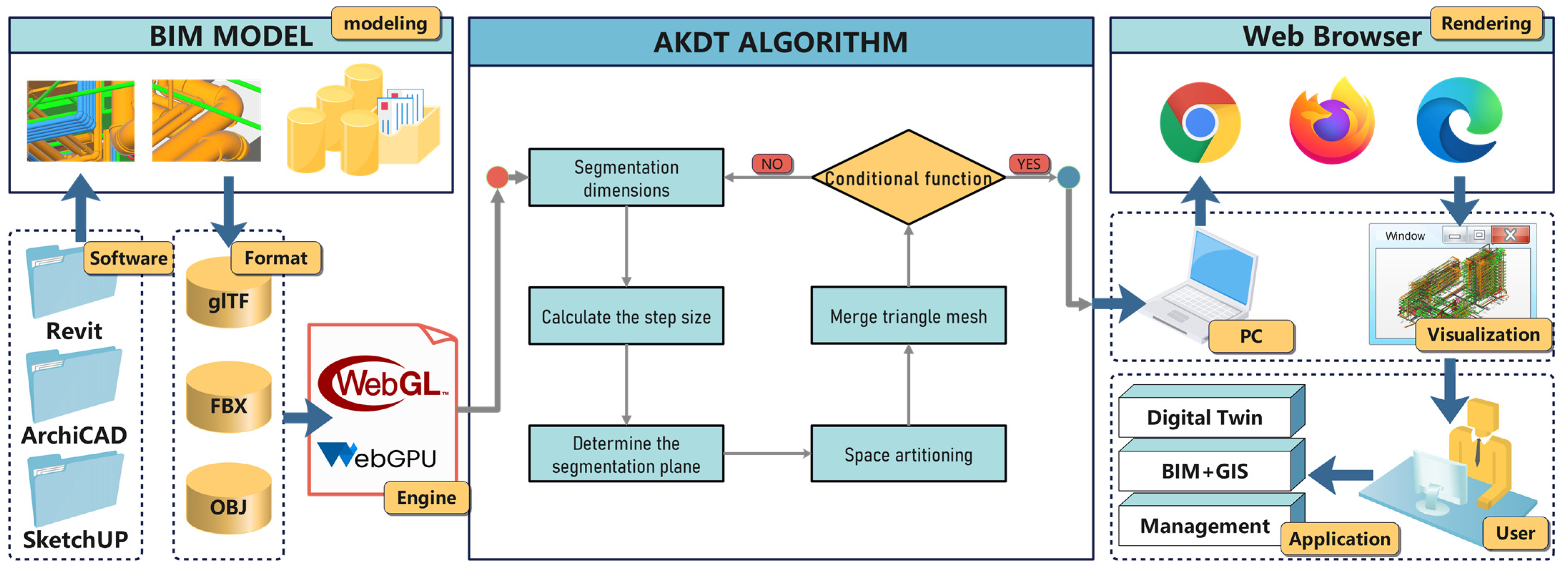
As illustrated in Figure 1, this study introduces the AKDT (Adaptive K-Dimensional Tree) algorithm, building upon prior research on traditional model rendering techniques and the K-D Tree. We conduct comprehensive experiments and analyses on the rendering efficacy of pipeline BIM models on web platforms using this algorithm.

The AKDT algorithm, as presented in this paper, initially employs the PCA method to compute model data. Based on these results, we can discern the model’s geometric features, and ascertain its primary expansion direction and layout, thereby determining a more efficient dimension division direction for rendering the pipeline BIM.

Moreover, the adaptive segmentation step size design allows the algorithm to tailor itself to the data density variations across regions, refining the segmentation procedure and enhancing the algorithm’s overall efficiency. We also introduce concepts of data density gradient and data heterogeneity, formulating an energy function to pinpoint the optimal segmentation hyperplane. Given the potential for redundant triangles generated during algorithmic segmentation, a merging strategy is proposed to maintain the BIM model’s geometric and semantic integrity and ensure model quality. A weighting function is then crafted to guarantee the algorithm’s timely termination, considering the web platform’s rendering capabilities. This ensures optimal rendering results while conserving computational resources.

By integrating these steps, the AKDT algorithm ultimately renders and optimizes the pipeline BIM model on web platforms.

2. Materials and Methods

2.1. Description of The AKDT Algorithm

As shown in Figure 2, the AKDT (Adaptive K-Dimensional Tree) algorithm in this paper is based on the further optimization of the BSP Tree (Binary Space Partitioning Tree). This algorithm first selects one of the 3D scene coordinate axes as the segmentation hyperplane, and then recursively divides the scene space of the pipeline BIM model according to the AKDT algorithm strategy. At the same time, the space can be divided dynamically according to the discrete degree of pipeline model data and spatial distribution pattern and other factors. In addition, the algorithm designs a termination condition function for the spatial division of the pipeline BIM model, which not only takes into account the amount of data, but also integrates key parameters such as the depth of the tree.

AKDT algorithm steps:

1.

Initialize to build the root node:

Generate a wraparound box that surrounds the pipeline BIM model in the view field as the root node. The orientation of this enclosing box is aligned with the coordinate axes.

2.

Space segmentation:

(1)

Spatial dimensioning: combining PCA methods to select segmentation axes.

(2)

Determine the adaptive segmentation step: dynamically calculate the segmentation step based on parameters such as the amount of BIM model data contained in the current node, spatial density, and the preset segmentation strategy.

(3)

Determine the segmentation hyperplane: determine the segmentation hyperplane according to the optimal segmentation hyperplane determination method.

(4)

Constructing subspace: Based on the segmentation hyperplane, the data space is divided into left and right subspaces according to the coordinates of the projection on the segmentation axis.

3.

Recursive subspace:

For the generated subspace, perform the space partitioning operation of step 2 again.

2.2. Segmentation of Dimensions Based on PCA

In order to ensure that the AKDT algorithm achieves optimal performance and accuracy when dealing with pipeline BIM models, the algorithm must select the appropriate segmentation dimensions in each recursive iteration. PCA (principal component analysis) is widely used to determine the main features of the dataset, and in this paper, we adopt the PCA methodology to determine the features of the model vertex distribution. Through computational analysis, we can determine the spatial distribution of model vertices in different coordinate axis directions, and then determine the division dimension. At the same time, the dimensional segmentation according to the direction of the model arrangement can minimize the subsequent impact on the model geometry during rendering and ensure the integrity of the model.

Segmentation of dimensionality steps based on PCA:

1.

Representation of datasets:

First, get the dataset of model vertex coordinates, denoted as $P$:

$$P=\left\{p_1,p_2,\dots ,p_n\right\}$$

where each point $p_i$ is represented in 3D space as

$$p_i=\left(x_i,y_i,z_i\right)$$

2.

Calculate the mean coordinates of the dataset:

Calculate the mean point by averaging the coordinates of each dimension $\overline{p}$ Coordinates of the mean point

$$\overline{p}=(\overline{x},\overline{y},\overline{z})$$

3.

Construction of covariance matrix:

Constructing the covariance matrix $C$:

$$C=\frac{1}{n}\sum _{i-1}^n \left(p_i-\overline{p}\right){\left(p_i-\overline{p}\right)}^T$$

(1)

4.

Calculate eigenvalues and eigenvectors:

Solve for the covariance matrix $C$ and the corresponding eigenvectors of the covariance matrix ${\lambda }_1,{\lambda }_2,{\lambda }_3$ and the corresponding eigenvectors $v_1,v_2,v_3$ of the covariance matrix.

5.

Determine the principal eigenvectors:

Find the largest eigenvalue ${\lambda }_{\mathrm{m}\mathrm{a}\mathrm{x}}$ Corresponding eigenvector $v_{\mathrm{m}\mathrm{a}\mathrm{x}}$:

$${\lambda }_{\mathrm{m}\mathrm{a}\mathrm{x}}=\mathrm{m}\mathrm{a}\mathrm{x}\left({\lambda }_1,{\lambda }_2,{\lambda }_3\right)$$

6.

Determine the segmentation dimension:

Based on the $v_{\mathrm{m}\mathrm{a}\mathrm{x}}$ component of the data to determine the principal direction of the

$$D=\left\{\begin{array}{ll}x& \mathrm{if} \left|v_x\right|\ge \left|v_y\right| \mathrm{and} \left|v_x\right|\ge \left|v_z\right|\\ y& \mathrm{if} \left|v_y\right|>\left|v_x\right| \mathrm{and} \left|v_y\right|\ge \left|v_z\right|\\ z& \mathrm{if} \left|v_z\right|>\left|v_x\right| \mathrm{and} \left|v_z\right|>\left|v_y\right|\end{array}\right.$$

(2)

where $D$ is the selected segmentation dimension.

2.3. Adaptive Segmentation Step

During the segmentation process, the AKDT algorithm uses an adaptive approach to dynamically adjust the segmentation step size according to the data density and data volume size of the current node.

In relatively sparse data regions, based on the low density characteristics of the data, fine-grained segmentation does not produce significant geometric detail gains, but leads to reduced query efficiency and increased storage resource consumption. Each newly generated tree node is accompanied by an incremental data structure maintenance cost, which increases the computational complexity of the algorithm. Therefore, in order to trade-off efficiency and accuracy, a larger segmentation step size strategy is adopted to avoid generating too many nodes, to achieve structural simplicity and save computational and storage resources.

In relatively dense regions of data, the use of too large a step size can lead to over-merging, making some of the details of dense data regions be lost. For this reason, a smaller segmentation step size is used, allowing the algorithm to perform finer subspace division in dense regions. This approach not only guarantees the realism and detail representation of the model, but also helps to balance the structure of the tree and further improve the efficiency of the algorithm.

Steps for calculating the adaptive segmentation step:

• Calculate the data density gradient:
  First, define the global data point collection $P_{\mathrm{global} }$, the total volume where the global data point collection is located $V_{\mathrm{global} }$, the number of global data points $N_{\mathrm{global} }$, the set of data points in the current subspace $P_{\mathrm{local} }$, the volume in which the local data point set is located $V_{\mathrm{local} }$, the number of local data points $N_{\mathrm{local} }$.
  Global average data density $D_{\mathrm{global} }$ and local data density $D_{\mathrm{local} }$ can be defined, respectively, as:

  $$\begin{array}{rr}& D_{\mathrm{global} }=\frac{N_{\mathrm{global} }}{V_{\mathrm{global} }}\\ & D_{\mathrm{local} }=\frac{N_{\mathrm{local} }}{V_{\mathrm{local} }}\end{array}$$

  (3)
  Gradient of data density $G$ is:

  $$G=D_{\mathrm{local} }-D_{\mathrm{global} }$$

  (4)
• Determination of Thickness Thresholds:
  Define $\beta$ as the deviation coefficient; calculate the threshold of consistency $\theta$, which is given by:

  $$\theta =\beta \times D_{\mathrm{global} }$$

  (5)
• Assessment of data heterogeneity:
  In order to assess the degree of dispersion of the data, for localized datasets $P_{\mathrm{local} }$, the standard deviation is calculated $\sigma$ with the formula

  $$\sigma =\sqrt{\frac{1}{N_{\mathrm{local} }-1}\sum _{i=1}^{N_{\mathrm{local} }} {\left(x_i-\mu \right)}^2}$$

  (6)
  Among others, the $x_i$ is the number of $P_{\mathrm{local} }$; the $\mathsf{\mu }$ is the mean value of the data points in ${\mathrm{P}}_{\mathrm{local} }$.
• Calculate the difference in data density:
  Calculate the data consistency difference $D$, data consistency gradient $G$, and the preset threshold of the denseness gradient $\theta$ difference between:

  $$D=G-\theta$$

  (7)
• Calculate the adaptive step size:
  Use the Sigmoid function to $D$ maps to the $(0,1)$ interval, where $k$ is a constant $S_{\mathrm{base} }$ is the base step size, and the adaptive step size $S$ is:

  $$S=S_{\mathrm{base} }\times \left(1-\frac{1}{1+e^{-\left(G-\theta \right)}}\right)\times \left(1+k\times \sigma \right)$$

  (8)

2.4. Optimal Segmentation Hyperplane Determination Methods

The Materials and Methods should be described with sufficient details to allow others to replica

Combining the data density gradient and the heterogeneity of the data, this paper constructs an energy function to evaluate possible segmentation points, which provides a mathematical criterion for determining the segmentation hyperplane and quantifies the quality of the segmentation to ensure that we can comprehensively assess the appropriateness of the segmentation points [30,31].

With the adaptive segmentation step, we select a series of candidate segmentation points, which are then evaluated using an energy function. Finally, the segmentation point with the lowest energy value is considered optimal, and combined with the previously determined segmentation dimension $D$, it is finally determined that the location of the segmentation point parallel to the $D$ dimension is the segmentation hyperplane.

Steps to determine the hyperplane

• Split the set of candidate points:
  Use an adaptive step size $S$ to select a candidate set of segmentation points, with $p_{\mathrm{start} }$ as the starting point on the dimension, and the set of candidate points $P_{\mathrm{samples} }$ is denoted as

  $$P_{\mathrm{samples} }=\left\{p_i\mid p_i=p_{\mathrm{start} }+i\times S,i=\mathrm{0,1},2,\dots \right\}$$
• Calculation of data density gradient:
  For the candidate segmentation point $p$, where $p\in P_{\mathrm{samples} }$, we first delineate a segmentation point centered on $p$ center and an adaptive segmentation step $S$ as the radius of the hypersphere. The data points contained in the hypersphere form the set $P_{\mathrm{local} }\left(p\right)$. The number of points is $N_{\mathrm{local} }\left(p\right)$ and the volume is $V_{\mathrm{local} }\left(p\right)$.

  $$\begin{array}{rr}& D_{\mathrm{global} }=\frac{N_{\mathrm{global} }}{V_{\mathrm{global} }}\\ & D_{\mathrm{local} }(p)=\frac{N_{\mathrm{local} }\left(p\right)}{V_{\mathrm{local} }\left(p\right)}\end{array}$$
  The gradient of data consistency $G\left(p\right)$ is defined as:

  $$G\left(p\right)=D_{\mathrm{local} }\left(p\right)-D_{\mathrm{global} }$$
• Assessing data heterogeneity:
  For the localized dataset $P_{\mathrm{local} }\left(p\right)$, we compute the standard deviation $\sigma \left(p\right)$, which is used to assess the data dispersion:

  $$\sigma \left(p\right)=\sqrt{\frac{1}{N_{\mathrm{local} }\left(p\right)-1}\sum _{i=1}^{N_{\mathrm{local} }\left(p\right)} {\left(x_i-\overline{x}\right)}^2}$$

  (9)
  Among other things, the $x_i$ is the number of $P_{\mathrm{local} }\left(p\right)$; the $\overline{x}$ is the mean value of the data points in $P_{\mathrm{local} }\left(p\right)$. the average of the a p data points in.
• Define the energy function:
  To find the optimal splitting point, we define the following energy function.

  $$E\left(p\right)=w_1\cdot G\left(p\right)+w_2\cdot \sigma \left(p\right)$$

  (10)
  Of these, $w_1$ and $w_2$ are the weights.
• Split hyperplane:
  The point with the smallest value of the energy function is the optimal segmentation point $p$:

  $$p=\arg \underset{p\in P_{\mathrm{samples} }}{\mathrm{m}\mathrm{i}\mathrm{n}} E\left(p\right)$$

  (11)
  The equation of the partition hyperplane is expressed as $D=p_D$ where $D$ is the adjudicated division dimension $D\in (x,y,z)$.

2.5. Redundant Triangle Mesh Merging Method

The Materials and Methods should be described with sufficient details to allow others to replica.

Consider that when spatially dividing a 3D model, the triangular facets that are split in the model form multiple smaller triangular facets. We consider re-merging these redundant triangles after segmentation.

First, redundant triangles are labeled, and when the segmentation is over, triangular facets with such labeling are looked up within the leaf nodes. Then, determine whether they can be merged based on whether they are adjacent and whether their normal vectors are the same. If the conditions are satisfied, we merge their shared vertices and update the data structure of the triangles.

Meanwhile, after the merging process, we also need to remove redundant triangles and update the index of triangles within the leaf nodes in order to ensure the consistency and accuracy of the data. In this way, we avoid excessive redundant triangles while ensuring the integrity of the model.

Steps to merge triangular facets:

1.

Marking redundant triangles:

Let the set of integral triangles be $T$. In the spatial division process, for any triangle $t\in T$, if it is partitioned, a new set of triangle segments is produced $T_{\mathrm{split} }^t$.

Set flags for redundant triangle facets: flag $\left(t^{\prime }\right)=$ split, $\forall t^{\prime }\in T_{\mathrm{split} }^t$.

2.

Labeled triangle segments merged:

All triangles within the leaf node are $T_{\mathrm{node} }$, where the set of labeled triangles is $T_{\mathrm{node} }^{\mathrm{split} }\subseteq T_{\mathrm{node} }$.

For the triangles in the $T_{\mathrm{node} }^{\mathrm{split} }$ triangles in the set, do the following.

(1)

Adjacent Triangle Determination:

For two triangles $t_1,t_2\in T_{\mathrm{node} }^{\mathrm{split} }$ the

Their adjacency conditions are denoted as:

$$\mathrm{Adjacent}\left(t_1,t_2\right)\iff E_1\cap E_2\ne \mathrm{\varnothing }$$

(12)

where $E_1,E_2$ are, respectively, the sets of edges of $t_1,t_2$.

(2)

Normal vector determination:

If $t_1,t_2$ are adjacent, then they have the same normal vector condition:

$$\mathrm{SameNormal}\left(t_1,t_2\right)\iff N_1=N_2$$

(13)

where $N_1,N_2$ are the normal vectors of $t_1,t_2$.

(3)

Vertex Merge:

If $\mathrm{A}\mathrm{d}\mathrm{j}\mathrm{a}\mathrm{c}\mathrm{e}\mathrm{n}\mathrm{t}\left(t_1,t_2\right)$ and $\mathrm{S}\mathrm{a}\mathrm{m}\mathrm{e}\mathrm{N}\mathrm{o}\mathrm{r}\mathrm{m}\mathrm{a}\mathrm{l}\left(t_1,t_2\right)$ are both true, then perform a vertex merge:

$$V_{\mathrm{merge} }=V_{1, \mathrm{shared} }=V_{2, \mathrm{shared} }$$

where $V_{\mathrm{merge} }$ denotes the merged vertices, $V_{1, \mathrm{shared} }$ and $V_2$, shared are the shared vertices of $t_1$ and $t_2$.

3.

Update leaf node data:

Clear the marking of triangles within leaf nodes: flag $\left(t^{\prime }\right)=$ none. $\forall t^{\prime }\in T_{\mathrm{node} }$ and remove redundant triangles and update the index of the triangle.

2.6. Termination Condition Weighting Function

To ensure that the algorithm stops under suitable conditions, a termination condition weighting function is designed in this paper. Starting with the amount of data in the node, if the number of data points within the node is too low, it means that there is no need to subdivide this node further. In addition, we also limit the maximum depth of the tree in order to avoid the negative impact of an overly deep tree structure on the computational efficiency. The data density gradient is also considered, which reflects the difference in distribution density between the local data and the overall data; if this difference is too small, there is no need for further subdivision. Data heterogeneity was also considered, and when the standard deviation was below a certain value, it indicated that the data in this region had homogenized and no further subdivision was needed.

Finally, the algorithm also takes into account the amount of change in the energy function; if the change in the energy function is small after several consecutive splits, it means that the splits will not have a significant effect. These weights express the importance of different conditions for the termination of the algorithm, ensuring that the algorithm can be terminated at the right time for optimal optimization.

1.

Node data volume:

If the amount of data in a node falls below a particular threshold, it is no longer subdivided. We remember that the number of data points in a node is $N$, then the termination condition is:

$$N<N_{\mathrm{m}\mathrm{i}\mathrm{n}}$$

where $N_{\mathrm{m}\mathrm{i}\mathrm{n}}$ is the preset minimum number of data points.

2.

Tree Depth:

In order to avoid computational inefficiency caused by a tree that is too deep, we set a maximum depth of $H_{\mathrm{m}\mathrm{a}\mathrm{x}}$. The current depth of the tree is $H$, and the termination condition is

$$H\ge H_{\mathrm{m}\mathrm{a}\mathrm{x}}$$

3.

Data density gradient:

Data density gradient $G$ can express the difference in distribution density between local and global data points. If the absolute value of $G$ is below a certain interval, it means that the data distribution in the region has been relatively uniform. The termination condition is

$$\left|G\right|<{ϵ}_1$$

where ${ϵ}_1$ is a predefined threshold for thick density gradient.

4.

Data heterogeneity:

The heterogeneity of the data can be represented by the standard deviation of the data $\sigma$ to indicate it. If the standard deviation of the data is $\sigma$, it is below a certain threshold; this means that the data are evenly distributed. The termination condition is

$$\sigma <{ϵ}_2$$

where ${ϵ}_2$ is the preset data heterogeneity threshold.

5.

The amount of change in the energy function:

The amount of change in the energy function $\Delta E$.

If $\Delta E$ (the amount of change in the energy function) is less than a certain threshold, it indicates that segmentation no longer leads to significant information gain, it indicates that the segmentation no longer leads to a significant information gain. The termination condition is

$$|\Delta E|<{ϵ}_3$$

where ${ϵ}_3$ is a preset broad value for the amount of change in the energy function.

6.

Termination condition function:

Define the following weights: $w_N$, $w_H$, $w_G$, $w_{\sigma }$, $w_E$ are the weights of the corresponding conditions, respectively.

The termination weighting condition function is.

$$F=w_N\cdot f_N\left(N\right)+w_H\cdot f_H\left(H\right)+w_G\cdot f_G\left(G\right)+w_{\sigma }\cdot f_{\sigma }\left(\sigma \right)+w_E\cdot f_E\left(\Delta E\right)$$

(14)

Finally, the termination condition is: If $F\ge \delta$, where $\delta$ is a preset threshold that can be set as desired. When the termination condition function $F$ is greater than or equal to $\delta$, the algorithm terminates.

3. Results

3.1. Experimental Setup

In order to verify the actual rendering effect of the AKDT algorithm on pipeline BIM models, we built an experimental environment for testing. On the server side, we configured hardware devices equipped with Intel Xeon E5-2630 processors dedicated to publishing BIM data. On the client side, we used a laptop equipped with i7-10875H CPU and RTX2060 GPU to observe the experiment.

In order to ensure that the experimental results could fully reflect the performance of the AKDT algorithm under different data sizes, we selected four pipeline BIM models for testing, as shown in

Table 1. Experimental dataset.

Data Name	Model Size	Number of Faces	Thumbnail
Office Building	126 MB	861,327
Outpatient Building	452 MB	4,946,136
Parking Garage	1043 MB	9,367,512
Urban Pipe Network	2067 MB	18,467,380

. We first tested the AKDT algorithm for its graphical rendering results. At the same time, its rendering effect is compared with the classical Octree algorithm. In order to quantify the performance of the AKDT algorithm, two widely used algorithms in the field of graphics, Octree and BVH (Bounding Volume Hierarchy) tree, are selected as control groups. Three key performance metrics, the initial loading time on the Web side, the change in frame rate during dynamic rendering, and the response time during interaction, are identified as the reference standards for evaluating the performance of the AKDT algorithm.

Ultimately, we provide a clear, structured, and quantitative assessment of the effectiveness of the AKDT algorithm in real-world applications through a series of comparative experiments.

3.2. Visualization Effects

In order to test the visualization of the AKDT algorithm in web browsers, experimental validation was performed. As shown in Figure 3, these data were rendered using the AKDT algorithm in combination with WebGL technology.

Meanwhile, under the condition of keeping the loading time constant, we compared the rendering effect of the AKDT algorithm with the traditional Octree algorithm. As shown in Figure 4, the results indicate that the pipeline BIM model optimized by the AKDT algorithm presents a clearer effect visually, and the overall structure of the model and the geometric structure of the edges are completely rendered.

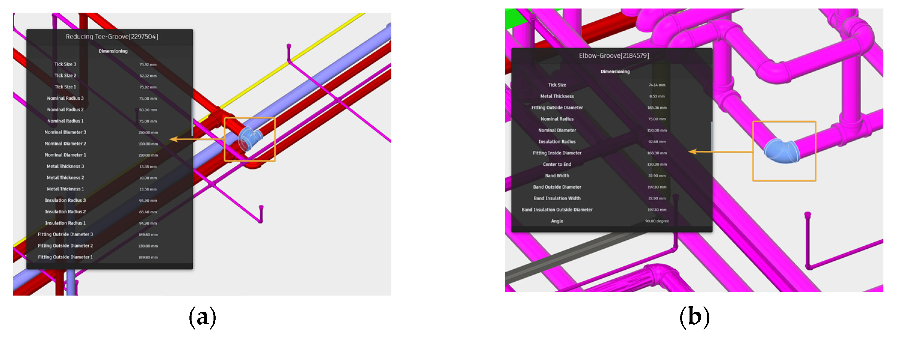
Further, as shown in Figure 5, after the BIM model has been spatially divided by the AKDT algorithm, the semantic information of the model can be completely displayed, and the parameters of the subcomponents are displayed normally.

We also brought the viewpoint closer and tested the visualization of the AKDT algorithm when dealing with large-scale and geometrically complex BIM models. As shown in Figure 6, the AKDT algorithm is still able to provide clear and accurate visualizations.

3.3. Comparative Analysis

3.3.1. Initial Loading Time

As shown in Figure 7, we used four datasets of different sizes and initialized the rendering in a web environment that kept the network bandwidth and computational resources consistent. The loading time measurements are timed from the beginning of the data request until the model is fully rendered on the screen to end the timing. The results show that the AKDT algorithm significantly outperforms the other two algorithms in terms of loading time, especially when dealing with large-scale datasets.

3.3.2. Frame Rate

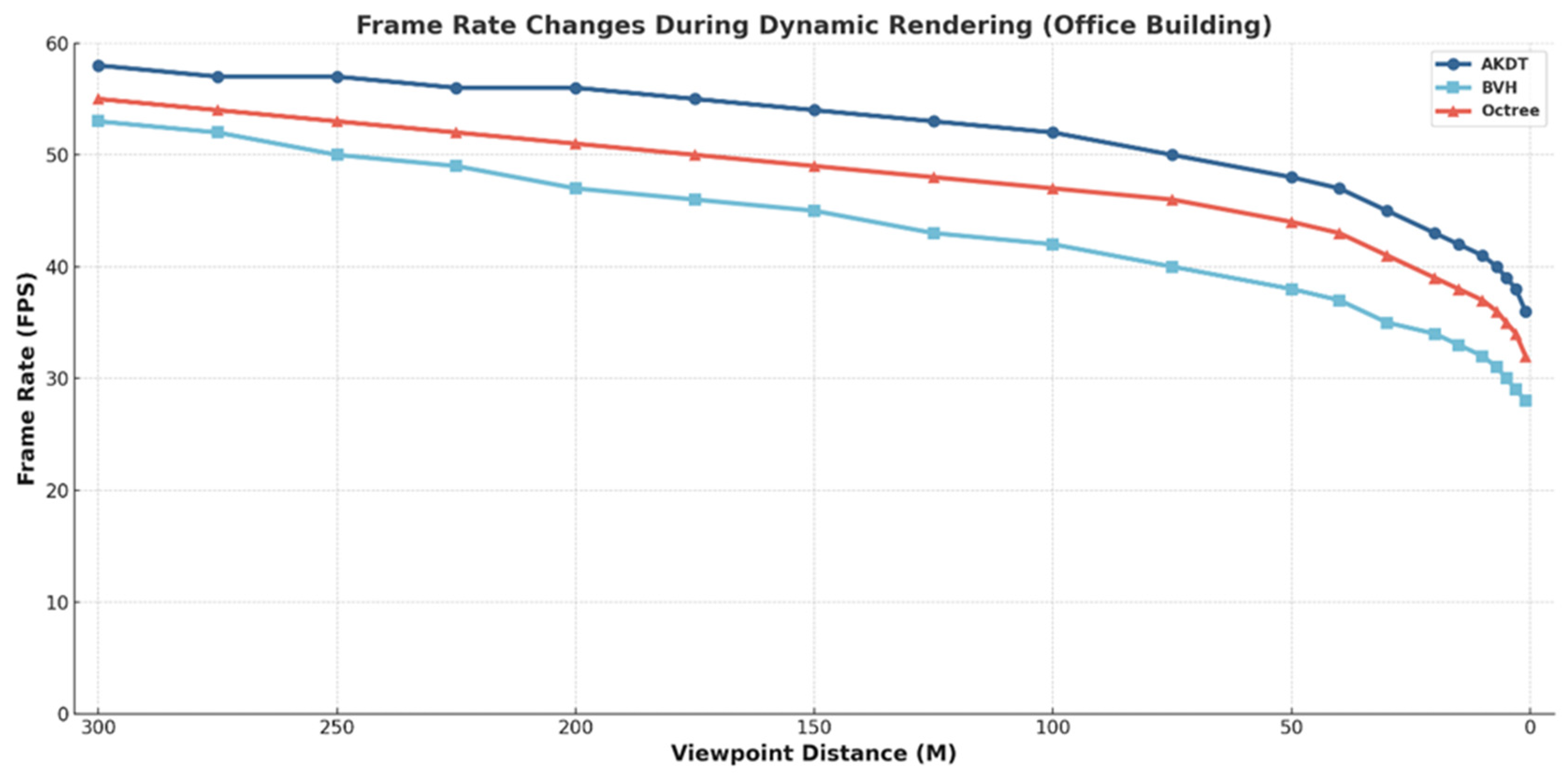
We used two pipeline BIM models, the smallest-sized outpatient building and the largest-sized urban pipeline network, as experimental data, and gradually reduced the viewpoints from a distance of 300 m to 1 m for the outpatient building model, and from a distance of 500 m to 1 m for the urban pipeline network model, and recorded the rendering frame rates at each specific distance point. The analysis of the results shows that the frame rate for all algorithms decreases with decreasing viewpoint distance for both data, which is due to the increase in model details in the view.

As shown in Figure 8, for the outpatient building data, the curve of the algorithm is smooth, and the AKDT algorithm is able to maintain more than 50 frames at a viewpoint distance of more than 100 m and around 40 frames at a viewpoint distance of less than 10 m compared to the other algorithms.

As shown in Figure 9, for the urban pipe network data, the frame rate fluctuates significantly because of the large model size and complex pipe structure. However, the average frame rate of AKDT algorithm is still higher than other algorithms, and it can keep more than 50 frames when the viewpoint distance is more than 300 m, and can still keep about 30 frames when it is 50 m.

The AKDT algorithm renders with a higher average frame rate and a smaller frame rate drop, indicating that it is better optimized and performs more stably in the face of viewpoint changes.

3.3.3. Interaction Response Time

As shown in Figure 10, in this experiment, we performed interactive operations such as rotation, scaling, and translation for different sizes of pipeline BIM models and compared the performance of the AKDT algorithm with other algorithms in terms of average response time.

By analyzing the experimental results, we observe that the AKDT algorithm provides faster response times at all dataset sizes. Regardless of whether the data are small or large, the AKDT algorithm responds more efficiently to interaction operations, resulting in a smoother and faster interaction experience with the model.

4. Discussion

This paper presents the AKDT algorithm, a Web3D rendering optimization algorithm for pipeline BIM models. The algorithm uses an adaptive strategy based on BSP Tree for spatial partitioning of pipeline BIM models, considering that the pipeline BIM model has special spatial characteristics, most of which are manifested as longitudinal or transverse linear structures. In the actual pipeline laying process, pipelines often follow a fixed spatial direction, and multiple pipe segments are arranged in the same direction with dense spatial distribution. This means that, compared with other BIM models, the vertices of the pipeline BIM model show significant denseness on the spatial coordinate axis, and the direction of the vertex distribution is highly fitted to the direction of the spatial coordinate axis.

Based on the above analysis, the AKDT algorithm first analyzes the optimal segmentation dimensions with respect to the geometric characteristics of the pipeline BIM. The goal of this strategy is to ensure that the segmentation hyperplane conforms to the main distribution direction of the underground pipeline BIM model. This strategy not only reduces the depth of the tree, but also improves the efficiency of the algorithm. Second, the segmentation step size is dynamically adjusted in the recursive process of the AKDT algorithm so that it can flexibly adapt to the data density and distribution of different regions and carry out meticulous spatial segmentation in dense regions, while avoiding excessive subdivision in sparse regions, so as to effectively optimize the segmentation process. In order to further optimize the segmentation effect, we introduce an energy function which combines the optimal segmentation dimension and adaptive step size to determine the optimal segmentation hyperplane. This process integrally considers the density gradient and heterogeneity of the data to ensure the uniform distribution of the data and the balance of the tree structure to achieve a reasonable adaptive effect. In addition, in order to maintain the integrity of the model, the generation of redundant data was avoided. We merged the redundant triangles generated due to segmentation. Finally, we designed a termination condition function that combines multiple factors to ensure that the AKDT algorithm stops at the right time, thus achieving the best optimization results and saving resources at the same time.

5. Conclusions

Experiments demonstrate that the algorithm proposed in this study offers significant advantages over traditional methods.

The AKDT algorithm’s rendering optimization ensures that the pipeline BIM model is vividly presented on the web platform. The entirety of the model’s structure, edge geometry, and semantic information remains intact. Notably, there is no loss in the model’s geometric or semantic details due to spatial segmentation.

In terms of initial loading time, the AKDT algorithm surpasses traditional methods. On average, it reduces the rendering time by over 11% across the experimental dataset. This efficiency is particularly evident with larger datasets, where the rendering time is reduced by nearly 18%.

When considering frame rate, tests conducted at different viewpoint distances indicate that the algorithm enhances the rendering frame rate by an average of over 8% for smaller datasets. This rate remains stable, averaging above 45 FPS. For larger datasets, the frame rate increases by an average of over 5%. However, there are some fluctuations due to the sheer volume of large data and the limitations of computer hardware, but the average frame rate is still over 30 FPS.

Regarding interaction response time, the AKDT algorithm proves to be faster. It reduces the interaction response time by over 14% compared to other methods. Furthermore, with larger datasets, the algorithm optimizes the response, cutting down the time by nearly 17%.

The algorithm’s efficiency in spatially managing pipeline BIM models enhances the visualization and browsing smoothness of these models on web browsers. This leads to optimized rendering. In practical applications, it can elevate the efficiency of staff operations, management, and maintenance of the pipeline BIM model. Additionally, the algorithm positively influences the development of digital twin technology and the integration of BIM + GIS.

However, there are areas for further optimization in this research. The algorithm is primarily designed as an optimization strategy for the geometric features of pipeline BIM models, making it ideal for rendering these models but somewhat limited for other BIM models. In addition, the study mainly considers rendering optimization on PCs. With the increasing use of mobile devices in practical applications, optimizing the rendering of pipeline BIM models on these devices is another aspect to consider.