Impact of Engineering Changes on Value Movement in Fund Flow: Monte Carlo-System Dynamics Modeling Approach

Abstract

A healthy fund flow system is crucial for the successful construction of any project. Project fund flow management has made significant progress, increasingly aligning with real-world applications. However, due to the uncertainties associated with Engineering Changes (ECs) in projects, the actual fund flow may still deviate from expectations. These systems still require improvements and corrections of flaws to enhance the efficiency of construction projects and reduce exposure to risks associated with ECs. Construction projects are complex and involve many processes. Each process represents a specific part of the project; therefore, an EC in one area can impact resource scheduling and fund balance. In our analysis, we found that ECs are directly related to fund demands and may result in the need for more materials, labor, and duration. Furthermore, ECs can alter construction progress and payment schedules, exacerbating project risks. As a result, effective management of fund flexibility becomes highly necessary. To explore the impact of ECs on the value dynamics of fund flow, it is important to understand and describe the stochastic paths of fund flow and discern the dynamic changes at each stage. Given this, we introduced a system dynamics model based on the Monte Carlo simulation. This model adeptly characterizes project risks and quantifies uncertainty variables, thereby making the simulation more aligned with reality. Moreover, the model illuminates the intricate relationship between project risk and project productivity, highlighting the origins of fund flow fluctuations. It is imperative to identify project risks early and address ECs promptly and effectively. Through sensitivity analysis and strategies, we ensure the stability of fund flow. This study offers a pivotal framework for understanding and managing fund flow in projects, emphasizing the central role of system dynamics in this process.

1. Introduction

The construction industry, as a vital pillar of the global economic fabric, continuously grapples with numerous challenges. A predominant factor contributing to the complexity of construction projects is EC. Stemming from technological progress, new requirements, or modifications to external factors, these changes can trigger fluctuations in fund flows. Substantiated by recent studies, these disruptions can deviate fund paths, resulting in project expense variations of 20% to 50%. Such fluctuations not only modify the value of fund flows but also transform their core structures. Consequently, predicting the path, scope, and risks of these changes, as well as their propagation, especially in the context of project size and market demands, has emerged as a paramount challenge within the construction industry. While traditional project management structures are valuable, such as CPM or PERT, their efficacy in delineating the dynamic interrelationships of funds remains limited.

To address this issue, the study introduces an innovative methodology that melds system dynamics with Monte Carlo simulations. This approach enables a more detailed simulation of fund flow paths following EC, factoring in potential internal feedback, time delays, and other kinetic variables. Incorporating Monte Carlo simulations into this model enhances the comprehension of the stochasticity and unpredictability induced by ECs. The primary goal of this research is to equip decision-makers with a robust experimental tool, empowering them to discern fund flows from a systemic perspective. This, in turn, bolsters their capability in predicting and managing the potential impacts of EC on fund flows, thus ensuring the smooth progression of projects. In summation, this study bridges a gap in the current research by offering a novel academic perspective and methodology. More critically, it provides tangible value to practitioners in the construction industry, steering them towards effectively managing the uncertainties of fund flows. Furthermore, a brief summary of the organisation is provided below for better comprehension of the content and structure of this study: In Section 2, the paper delves into existing approaches for fund management under uncertainty, as well as their applications in the field of system dynamics. Following that, in Section 3, a model is constructed to describe the movement of fund value caused by ECs by incorporating both the Monte Carlo technique and the concepts of system dynamics. In Section 4 then uses the Yangfanggou Hydropower Station as a case study to model fund value flow scenarios and conduct sensitivity analysis. Finally, in Section 5, conclusions are formed and new study directions are recommended.

2. Literature Review

2.1. Engineering Change

EC has become a vibrant area of study and development, attracting more and more interest from the academic world and the building sector; see Jarratt et al. [1]. A comprehensive definition of EC is necessary before conducting problem-oriented research in this area. In light of the development of engineering change definitions throughout time, Williams et al. [2] provided one of the early definitions of EC, which refers to changes made to a product’s components after it has gone into production. According to Barrie and Paulson Jr. [3], EC typically includes revisions to the initial contractual scope, changes to project procedures, variations to the anticipated completion date, and adjustments to prices. EC, according to Thomas and Napolitan [4], includes any alterations to the project’s original scope. A reminder is provided by Hanna et al. [5], who defines an EC as any occurrence that modifies the project’s original scope, projected budget, and timetable. It is clear that academics have presented minor differences in how they have described the first breadth of technical change. Hamraz et al. [6] provided a comprehensive definition, building on the foundation primarily established by Jarratt et al. [1], that covers changes or modifications to the structure, behavior, functionality, and relationships between functionality and behavior of technical artifacts. Thus, it is clear that managing EC will be a difficult undertaking given how it affects a project’s cost, quality, and schedule, among other factors. From the perspective of origin, ECs in construction and installation projects are primarily attributed to design negligence or errors (65%), design changes (30%), and unforeseen conditions (5%).These changes result in significant costs, with statistics indicating that ECs constitute 5% to 10% of the total project cost. In some cases, the cost of changes can exceed 30% of the total project cost [7]. On the other hand, as a result of their stochastic nature and facile dissemination, engineering modifications have the potential to transpire at any juncture throughout the entirety of the construction process [8]. Engineering modifications have a discernible impact on the fund flow movement effect in two distinct manners: initially, alterations in engineering will have an effect on the primary pattern of fund movement, and this effect will persist over time. As time elapses, the cumulative influence of ECs on the lag in fund flow becomes more pronounced [2]. Engineering modifications will have an impact on the fund flow utility’s worth, leading to discounted variations in the monetary value of funds at distinct junctures in time (fund value fluctuations). The matter of making trade-offs and adjustments to the interterm movement patterns of project funds inflow, outflow, and storage subsequent to significant engineering modifications to enhance the performance of project funds utilisation and avert the possibility of fund chain breakage is a crucial concern that demands the attention of decision-makers.

2.2. Project Fund Flow

The fund flow is critical in influencing the economic effectiveness of projects. This is especially true for contractors. The beginning and end of fund flow reveal the entire cycle of their economic activities [9]. Significant support from funds is required to guarantee a smooth transition from project inception to completion, catering to expenses, cost control, risk management, and change adaptation. However, projects have inherent uncertainties. Remarkably, ECs during construction have become the norm. While some ECs may enhance the value of a project, they can also incur additional costs and cause delays [10]. Against this backdrop, the concept of “value movement” takes on added significance. It is not simply a transfer of funds or resources within the project. Further investigation reveals that “value movement” is a multi-layered and multi-dimensional notion. It includes the funding sources, directions, the magnitude and direction of flows, the time dimension, and the interplay with other critical project variables. This insight assists us in determining how funds are efficiently allocated. It ensures that these flows align with the project’s objectives. Consequently, the “value movement” within these flows is the primary predictor of economic benefit. Because ECs are unpredictable and complicated, the demand and supply of funds can shift rapidly. In light of this, decision-makers must conduct a comprehensive analysis of the “value movement” in fund flows. Such insights will surely aid in better managing the impact of ECs, ensuring that the project stays on track with the budget and timeline.

In 1977, Ashley and Teicholz [11] proposed a cost-based strategy for fund flow management. This approach involves the direct categorization of costs into distinct categories such as labor costs, machinery and equipment costs, material costs, and other related expenses. The determination of the proportion of these cost categories in relation to the overall cost is made prior to the budgeting process. Sears [12] introduced a method for integrating schedule and cost items, which was further developed in subsequent studies. However, this approach did not account for the timing of expenditures and cost payments. In real-world applications, a temporal gap often exists between the occurrence of costs and their corresponding expenditures, resulting in notable discrepancies in the allocation of financial flows and a diminished precision in their implementation. The period after the reference “Park et al. [13]” is unnecessary and disrupts the flow of the sentence in formulating a model for cash inflow and outflow, with emphasis on the viewpoint of the general contractor. The cost weights are revised in accordance with the factual values of individual cost components, while simultaneously taking into consideration the influence of payment frequencies. As proposed by Görög [14], this serves as a representation of the cumulative cost fund flow for a given project. The model undergoes a gradual extension process, starting from a singular contractual agreement and eventually encompassing the entirety of the project’s lifecycle. The S-curve has been utilised by numerous scholars to examine the financial progression of engineering endeavours. Several mathematical model equations for the S-curve have been proposed by Jarrah et al. [15]; these methodologies rely on regression analysis of numerous finalised projects and the resolution of parameters to construct mathematical models, thereby showing limitations in their universal applicability.

2.3. System Dynamics

The field of engineering construction is subject to numerous influencing factors, rendering it a highly stochastic and unpredictable domain. Moreover, the analysis and study of fund flow in this context pose significant challenges, as simplistic mathematical analytical models are inadequate for this purpose. The expeditious advancement of the system dynamics simulation technique offers a propitious approach to address this issue. The aforementioned tool is founded upon the principles of system dynamics theory and serves as an analytical instrument for examining the behavior and interactions of a given system. Mathematical models are constructed to simulate and predict the behavior of a system, with the dynamics of the variables within the system being simulated. The field of system dynamics was initially conceptualised by Professor Jay W. Forrester, and subsequently applied to the analysis of business and societal systems [16]. Cooper [17] utilisation of system dynamics models to quantify the factors contributing to cost overruns in a military ship project in 1980 is widely recognised. System dynamics has been frequently utilised by scholars in their respective regions/countries for their research endeavours. Incorporating system dynamics into the microscopic realm of construction enterprise project cost control system, He and Cheng [18] conducted a comprehensive analysis of the management activities of construction enterprises for individual construction projects from a systematic perspective. This involved the flexible integration of various influencing factors associated with a particular strategy, in order to conduct a holistic investigation of construction enterprise project cost control. The interdependent relationship between project schedule and cost management is demonstrated by Liu and Yang [19] through the development of a system dynamics model. The authors subsequently determine the level of schedule control intensity that can be achieved while maintaining fixed costs. They ultimately suggested employing suitable techniques for schedule control to regulate costs and maintain a consistent level of control. Additionally, the degree of schedule control could be adjusted by monitoring fluctuations in the level of cost control, thereby preserving the stability of the system. Considering the matter at hand, we initially employ the system dynamics approach to examine the dynamic progression pattern of EC fund flow from a causal perspective and elucidate the flow mechanism of fund network. Additionally, we develop a value movement model of EC fund flow, which is integrated with the Monte Carlo stochastic simulation technique to depict the course of construction resource consumption [20]. We create distinct EC scenarios, evaluate the alteration degree of fund reserve, and identify the impact of engineering change uncertainty on project fund flow. Furthermore, the research employs sensitivity analysis to investigate the primary control factors of EC fund flow and its regulation level.

3. Proposed Approach

3.1. Characterization of Fund Flow under ECs

Contractors must create a precise cost plan before starting a project. During the intended term, this plan should explicitly detail predicted production expenses, cost levels, and cost reduction rates. Importantly, this plan serves as a cornerstone for financial management and accounting. As the project enters the construction phase, contractors establish an inventory based on completed work and submit payment requests to the client. Once the client reviews and approves the work, they pay the contractor within the specified time range. The contractor bears all financial burdens until the project reaches its financial settlement. The balance between funds supply and demand changes dynamically throughout the construction process, manifesting as a sequential fund flow pattern. Contractors must ensure efficient deployment of resources such as labor, materials, and machinery to accomplish this. However, factors such as design oversights, omissions, and shifting client requirements can lead to ECs, negatively affecting the project’s efficiency [21]. ECs can disrupt planned processes, prompting resource reallocation and potentially reducing work productivity. Furthermore, since ECs often require additional time, they might delay the overall project timeframe and expected income. This delay can accelerate fund outflows and decelerate inflows [22]. To tackle these challenges, contractors need to accurately estimate and deploy resources, and they should also maintain adequate fund reserves to cover potential shortfalls. The project’s fund flow essentially captures the timing of supply and demand. As a result, ensuring the consistency and stability of fund flows is critical to success. Figure 1 shows the causal relationship of fund flow under ECs.

Figure 1 illustrates the project’s fund flow, which displays the features of inflows and outflows over time. This flow is shaped by the supply and demand. The fund supply typically encompasses progress payments, claims, and compensatory loans, among other sources. Conversely, fund demand mainly consists of labor costs, material costs, mechanical equipment costs (including depreciation), and administrative fees. When allocating construction resources for a project, differences between the fund’s supply and demand cause fluctuations in the reserves. These disparities prompt funds, possibly from external sources, to flow into the reserve pool. Subsequently, these funds are redistributed to the project, generating a conservation cycle. Within this conservation cycle, the volatility of the fund reserves is directly influenced by the supply and demand. A surplus in the fund supply leads to an increase in the reserves, whereas an increase in fund demand results in a decrease.

During project execution, ECs are common and can potentially alter the fund’s supply and demand [9]. For instance, delays caused by ECs might influence the disbursement of progress payments, reducing the fund supply. Simultaneously, such ECs might lead to a decline in project productivity, increasing the demand for materials and labor, thereby amplifying the fund demand. Consequently, ECs often result in a reduction of fund reserves. Factors determining the dynamic nature of the supply include actual project progress, payment terms, contractual requirements, and project productivity rates. These factors drive fund inflow, providing positive feedback to the reserves. Conversely, construction progress, resource consumption rates, loan interest rates, and payment delays influence the dynamics of fund demand. These variables act as driving forces for fund outflow, exerting pressure on the fund reserves. In summary, the balance of the fund reserves serves as the primary constraint for project fund adjustment.

3.2. Key Assumptions of the Model

The creation of a system dynamics model serves the objective of modeling various ECs in order to investigate the shifting trends of fund flow dynamics. This study aims to quantify the impact of EC uncertainties on the value of project funds. To summarize the essence of this concept, consider the following key assumptions:

• The cost disbursements are normalized in reference to their timing [23].
• The stability of project fund origins remains unaffected by impediments such as loan difficulties.
• Fund interest rate stability remains throughout time, unaffected by temporal or other effects.
• ECs are observed to follow a normal probability distribution, with each alteration event being independent.
• Contractors consider unforeseen occurrences to be outside the scope of the system and so do not consider them.
• Despite increased costs, time extensions, or resource limitations as a result of engineering changes, the project’s continuity remains unbroken.

3.3. Model Building

Our research indicates that the fund flow system exhibits various sophisticated dynamic structures. Based on our previous examination of fund flow value features under ECs, variables in the system display causal linkages, temporal lags, and nonlinear interactions. System dynamics is a powerful tool for navigating such complexities. Furthermore, the concept of a simulated environmental laboratory is consistent with system dynamics, as it provides a platform for manipulating environmental factors to simulate various scenarios and monitor system responses. This, in turn, provides decision-makers with a better understanding of system behavior, guiding them toward resource allocation optimization.

The dynamic mechanism of the fund flow system essentially replicates the interaction between fund supply and demand [24,25]. Variables within each subsystem interact with one another, and the total system is organised into three subsystems: the reserve fund, the EC costs, and the EC index. The primary sources of funding supply are progress payments and loan schedules, while those for funding demand are EC costs and planned costs. This paper divides the EC costs subsystem into five types of expenses: labor change cost, material change cost, machinery change cost, auxiliary change costs (including transportation cost and fuel cost), and other change costs (including change management cost and depreciation change cost). According to Fang [26], ECs are primarily influenced by elements such as risk level, occasional risk factors, and management experience, which are mostly reflected in project productivity and project delay. Following an EC, project resources will be shifted, limiting project productivity; in addition, ECs may cause work disruptions, resulting in project delay. Through our analysis, we have developed a fund flow model driven by ECs, as illustrated in Figure 2. Specific variables and definitions are provided in

Table 1. Fund flow driven by EC: system variable analysis.

Number	Variable Name	Variable Definition
1	Reserve Fund	Reserve funds are used for unforeseen situations in a project.
2	Engineering Change Costs	The amount of cost change caused by engineering changes.
3	Funding Supply	Funding sources available for the project.
4	Funding Demand	The amount of funds needed for project execution.
5	Engineering Change Increment	The amount of change in project modification costs.
6	Progress Payment	Payments linked to project progress.
7	Loan Schedule	Repayment plan and scheduling for loans.
8	Planned Cost	The predetermined cost plan for the project.
9	Retention Ratio	The percentage of payments retained as a guarantee for subcontractors during project progression.
10	Payment Extension	The situation of delaying payments.
11	Project Delay	The actual completion time of the project exceeds the planned schedule.
12	Delay Handling Time	The time required to assess and process change requests.
13	Funding Interest Rate	The interest rate of loans.
14	Project Scale	The scope, size, and complexity of the project.
15	Occasional Risk Factors	Risk factors that may infrequently but significantly impact the project.
16	Management Experience	The experience and expertise of project management team members.
17	Risk Level	The degree of uncertainty and risk faced by the project.
18	Engineering Change Index	An index measuring the frequency and magnitude of engineering changes in a project.
19	Project Productivity [27]	The amount of work completed within a specific time, reflecting project efficiency.
20	Technical Complexity	The complex technologies and processes involved in the project.
21	Risk Tolerance	The organisation’s or project’s ability to tolerate risks.
22	Magnitude of Change	The extent and magnitude of the impact of changes on the project.
23	Expected ROI	The expected rate of return on investment, usually expressed as a percentage.
24	Machinery Change Cost	The additional costs caused by changes in machinery.
25	Auxiliary Change Cost	The additional costs caused by changes in auxiliary production.
26	Other Change Cost	The costs brought about by changes other than those mentioned above.
27	Labor Change Cost	The additional costs caused by changes in labor.
28	Material Change Cost	The additional costs caused by changes in materials.
29	Machinery Cost per Unit Time	Cost of machinery per unit of time.
30	Transportation Cost	Transportation-related costs.
31	Transportation Allocation Rate	Ratio of cost allocation to transportation expenses.
32	Fuel Cost	Fuel-related costs.
33	Fuel Energy Distribution Rate	Ratio of fuel energy allocation to various costs.
34	Change Management Cost	Costs required for managing project changes.
35	Depreciation Change Cost	Additional costs caused by depreciation changes.
36	Depreciation Cost Rate	Ratio used to measure the gradual decrease in value of fixed assets (such as equipment) over time.
37	Wage Rates	Labor price per unit of time, related to the scarcity of job types and market demand.
38	Miscellaneous Expenses	Other costs related to transportation, materials, etc.
39	Purchase and Storage Rates	Rates for material procurement and storage.
40	Engineering Change Increment	Increment of project progress and cost due to changes.
41	Labor Hours Change	Changes in labor hours due to changes in project quantities.
42	Construction Material Change	Changes in construction materials due to changes in project quantities.
43	Machinery Shift Change	Changes in machinery shifts due to changes in project quantities.

.

In Figure 2, the green variables represent the EC costs subsystem, the red variables correspond to the EC index subsystem, and the blue ones denote the reserve fund subsystem. The arrows in the diagram indicate the mathematical relationships between the variables. Table 1 presents the variable names and variable definitions in the model. The variables in the model are classified into subjective and objective parameters. Subjective parameters are estimated based on expert opinions and scholarly research, such as management level and risk tolerance [28,29]. On the other hand, objective parameters are assigned referencing national standards, historical data, and literature, such as wage rates and procurement fees [30]. The phrasing is a little vague; consider clarifying what is meant by “using tabulated functions”. To handle data assignment and equation formulation, three distinct processes have been executed:

• Because certain variables in the model have different dimensions, a method of function mapping or scaling by multiples has been adopted to control them within the same order of magnitude.
• According to the reinforcement theory in behavioral economics, positive rewards influence human activities, causing them to be repeated, while negative reinforcement causes them to diminish. In this article, the decision-maker’s risk tolerance is introduced as a critical factor. When the reserve fund is greater than zero, the decision-maker chooses to extend the processing time for engineering changes, resulting in a risk tolerance setting of 1.1. Conversely, when the reserve fund is not greater than zero, the processing time is reduced [31].
• Change probabilities remain within a distribution range with a positive probability density and a unimodal shape. This property is shared by probability distributions such as the normal distribution, the Beta Distribution, and the triangular distribution. Empirical evidence shows that the normal distribution accurately describes the distribution characteristics of variables [32].

4. Simulation Analysis

4.1. Fundamental Data

Yangfanggou Hydroelectric Station is located in the middle reaches of the Yalong River in the Liangshan Prefecture, serving as a core project for the cascade development of the middle reaches of the Yalong River. The study replicates fund flow by focusing on the 11th dam segment of Yangfanggou Hydroelectric Station. The project is planned to last three years, with the time unit being a quarter and the fund unit being CNY ten thousand.

Table 2. Comparison of progress payment and planned costs.

Time	1	2	3	4	5	6	7	8	9	10	11	12
Progress Payment	52.00	103.99	150.03	231.15	335.96	426.01	441.86	375.92	297.00	198.05	120.02	52.00
Planned Costs	70.31	120.24	182.54	250.61	385.25	486.25	513.19	438.44	331.23	220.12	130.48	67.34

documents the quarterly progress payment and planned costs.

4.2. Model Validation

Before initiating the simulation analysis, it is imperative to comprehensively validate the constructed system dynamics model. The methods for validating the model primarily encompass mechanical error checks, steel quantity consistency tests, and structural behavior evaluations. After testing, this model has successfully passed the mechanical error checks and steel quantity consistency tests using the Vensim PLE 10.0.0 Structural behavior evaluations mainly involve extreme value checks and sensitivity analysis, with this study specifically conducting sensitivity tests on certain parameters.

Within the analysis of the funding supply structure, the fluctuation in the retention fund ratio is seen as a pivotal factor affecting the status of the fund supply. To verify the model’s accuracy, we conducted 4000 simulations on the retention fund based on predefined values (MIN = 0, MAX = 0.1, MEAN = 0.5, DEV = 0.07). Figure 3 simultaneously illustrates the impact of the retention ratio fluctuations on the funding supply.

Figure 3 illustrates a confidence interval analysis of the impact of changes in the proportion of retained funds on fund supply. The central yellow region in the figure contains 50% of simulation outcomes, showing the most likely forecasts within this range. Additionally, the area encompassing both the central layer and an outer layer covers 75% of the simulation outcomes, exhibiting a broader range of probabilities. When extended to the central two layers and an outer layer, it covers 95% of the simulation outcomes, representing the effective range of fund supply. Finally, the operational results exhibit numerical sensitivity, since changes in the proportion of retained funds affect fund supply, although the curve lacks a clear trend. Thus, the coefficient setting in the model for the fraction of retained funds is reasonable, and the operational results have survived sensitivity testing.

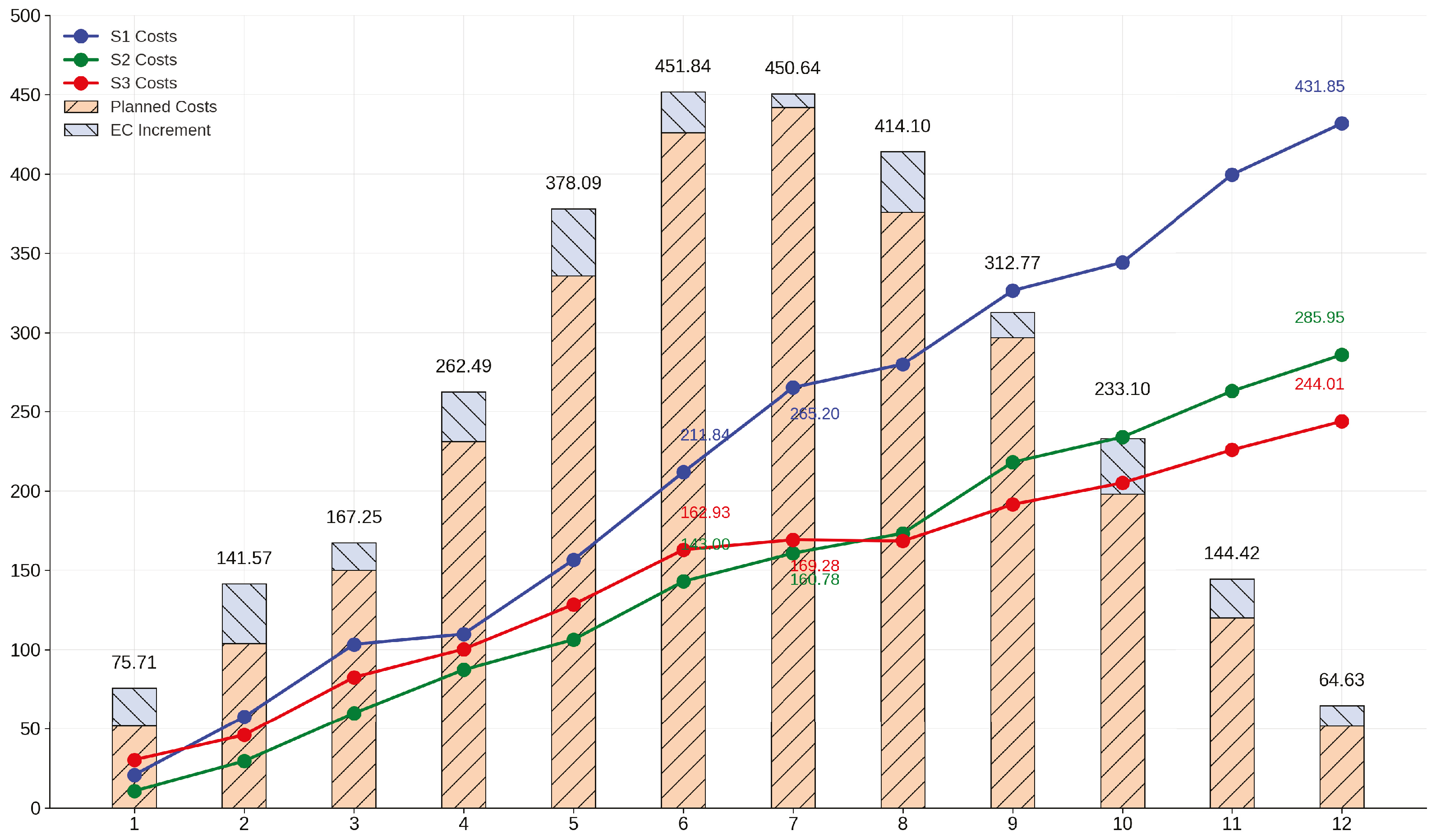
4.3. Fluctuation Patterns and Risks of Fund Flow Value under ECs

Upon inputting parameters into the model, the simulation duration is set for three years. However, this duration can be adjusted according to the project. Time parameters are measured in quarters. The Monte Carlo method is used to simulate three EC scenarios: S1, S2, and S3. Specifically, S1 replicates ECs at a high risk level, depicting scenarios when management’s capacities are relatively weak and the likelihood of facing occasional risks is higher. In contrast, S2 and S3, respectively, simulate EC scenarios under medium and low risk levels. Notably, the risk associated with ECs significantly diminishes in the S3. Based on this, we have established a link between risk levels and the potential range of changes: the higher the risk level, the greater the possible magnitude of the ECs.

The simulation results for these scenarios are depicted in Figure 4, Figure 5 and Figure 6. Figure 4 depicts the amounts of the ECs under the three scenarios (S1, S2, and S3). Within these scenarios, the mean/standard deviation of the EC amounts are 34.58/16.59, 23.13/9.67, and 19.19/10.94, respectively. Moreover, the maximum EC amount reaches 55.25 (S1, T = 5/10), while the minimum drops to −0.84 (S3, T = 7). This trend distinctly demonstrates that the project risk level correlates with, and majorly impacts, the EC amounts. Therefore, the experience of management and the occurrence of occasional risks are vital factors affecting the project’s ECs. However, in the early stages of the project’s building (T = [0,4]), an unexpected occurrence emerges: while the risk levels are S1 > S2 > S3, the EC amounts are either S2 > S1 or S3 > S1 (T = 2, S3 > S1; T = 4, S2 > S3 > S1). There are three plausible explanations for this phenomenon. First, the costs of design changes and revisions during the early project phases are relatively modest, making the relationship between project risk levels and EC amounts less evident. Second, risk identification and management measures may have an impact on the amount of ECs. Early detection and early response can significantly reduce EC levels. Lastly, the allocation and style of resource utilisation may have an impact on the project risk level. Investing additional resources may raise the risk level, but having an abundance of resources might help to speed adjustments.

Drawing from the data in Figure 4, we delved deeper into the cumulative trends of EC costs and fund reserves. Figure 5 and Figure 6 show the results of the simulation. Figure 5 displays the continual accumulation of EC costs, with the bar graph displaying these amounts (highlighted in light blue) based on average data from three different scenarios. In the early stages of the project (T = [0,6]), the accumulation of EC costs displays a trend of S1 > S3 > S2. Surprisingly, during the T = [7,8] time frame, S2 eventually overtakes S3 over time. As time progresses, S2 gradually overtakes S3, culminating in a final sequence of S1 > S2 > S3. By correlating with Figure 4, it becomes evident that at T = 7, the EC amount for S3 is negative. This factor, in turn, slows the rate at which the EC costs accumulate, relieving strain on the fund chain. Shifting our focus to fund reserves, as shown in Figure 6, within the T = [0,7] period, the cumulative value of fund reserves is negative, signified by a slope of less than zero. This indicates a discrepancy in fund supply and demand during this phase, suggesting that the funds’ ability to handle risk is compromised. Consequently, project decision-makers must pay special attention to mitigating unknown risk factors. Moreover, there is a pressing need to bolster the project’s risk reserve funds to counteract the adverse effects from ECs. Considering the time value of funds and assuming an industry investment return rate of 10%, when the EC amount reaches 8.28% of the contract price, the project’s funds will achieve a break-even point. This means that contractors expect 8.28% as the project’s representative change level.

4.4. Sensitivity Analysis

In the system model presented, which covers the movement of funds under ECs, the disparity level of the reserve fund serves as a primary constraint for adjusting project funds. To ensure system stability, decision-makers must precisely identify and subsequently refine the major parameters that influence the form of the fund value. Consequently, this section digs into a sensitivity analysis of these predominant factors. However, while conducting a sensitivity analysis on a specific parameter, other parameters remain constant. Furthermore, by changing the value of the parameter under consideration, we can ascertain its impact on the reserve fund. As shown in Figure 4 and Figure 5, one strategy for adjusting fund reserves is to mitigate potential project risks. Project scale, management experience, and contract rates were all decided during the genesis phase as proactive control measures. Given this, it is critical to emphasise the consequences of delayed processing time in order to refine and optimise fund reserves.

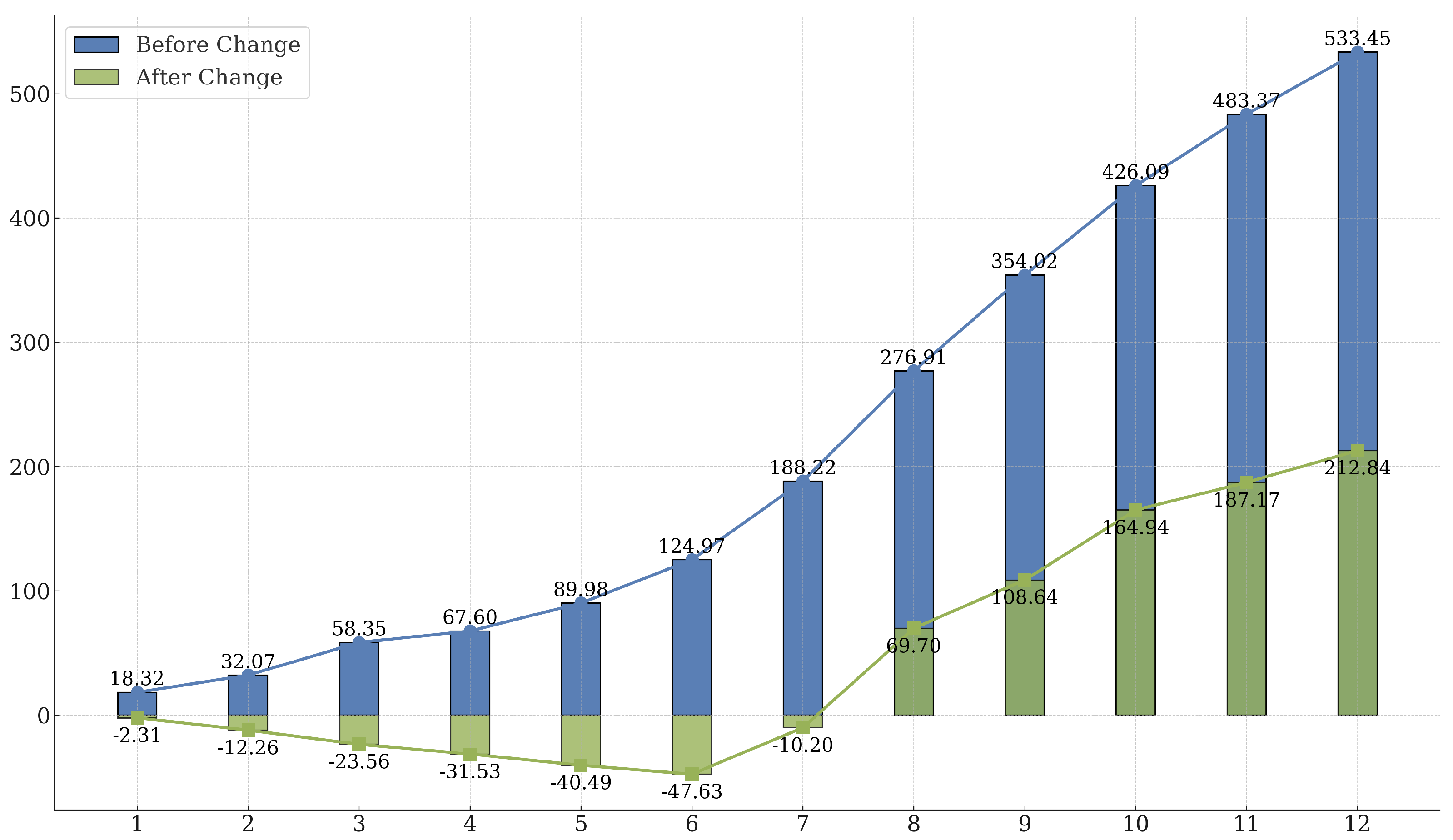
4.4.1. Impact of Delay Handling Time Changes on Fund Reserves

Delay handling time refers to the time lag between the identification of an EC request and the decision-making process. Such a delay could occur as a result of limited resources, ineffective information flow, or other factors. When ECs occur, the delay handling time has a substantial impact on the form of fund value, potentially affecting project productivity and resulting in project delays. Consequently, keeping all other parameters constant, we chose a range of delay handling times for simulation, specifically T = 1, 3, 5, 7. The four scenarios are denoted as: Case1@delay1, Case2@delay3, Case3@delay5, and Case4@delay7. Figure 7 depicts the simulation findings.

Figure 7 illustrates the changes in delay handling time with time (T = [0,12]) for four different scenarios (from case1 to case4). A discernible trend is that the reserve funds of the project undergo two phases. The reserve funds consistently decrease during the negative growth phase (T = (0,7)). Notably, the decline in Case4@delay = 7 is the most pronounced in this phase, whereas the decrease in the other three situations is more gradual. However, once we enter the positive growth phase (T = [8,12]), the reserve fund begins to rise. Case1@delay = 1 exceeds the others in terms of growth rate, whilst Case4@delay = 7 falls behind. Further investigation reveals that the reserve funds for Case4@delay = 7 during the mid-project phase are significantly smaller than those for the other three cases. In summary, given the occurrence of engineering changes, as the delay in handling time increases, the fluctuations in funds intensify, requiring a longer duration to achieve a balance in supply. When the time intervals are consistent, the later the delay in handling time, the more pronounced the impact on the cumulative value of fund reserves. The effects of the delayed handling time on fund flow are most visible in three facets. Firstly, it may incur higher EC charges, increasing the outflow of funds. Secondly, project delays might defer progress payments, resulting in a decrease in fund inflow. Thirdly, certain contracts might have penalty clauses for project delays. Consequently, the delay handling time has a major effect on the project’s fund flow patterns. This could result in a scenario where the original budget falls short, forcing the infusion of more funds into the reserve. The balance between funding supply and demand changes further into the future as the delay handling time increases. Furthermore, as time progresses, the reserve fund gap grows, creating significant obstacles to the project’s long-term viability.

In analyzing how project delay handling time affects different stages, during the early stages, ECs are often minimal and manageable, owing to the fact that the bulk of the work has not commenced. However, ignoring changes at this stage can lay the ground for greater changes later on, incurring higher costs and time overruns. Midway through the project, as the primary tasks are underway, any changes can result in redoing completed tasks. This not only raises costs but may also cause project delays. Addressing adjustments becomes critical throughout the project’s final stages. Given that the majority of the work has already been completed, any changes can result in massive rework, significantly driving up both costs and delays. Therefore, as the project matures, the costs associated with ECs increase. It is prudent to conduct a full risk assessment early on and to respond to ECs as they develop, reducing cumulative risks and EC-related costs. To reduce delay handling time, it is beneficial to implement a defined change management approach from the start of the project. Notifying important stakeholders as soon as possible after receiving change requests ensures that everyone is on the same page, eliminating misunderstandings and avoiding duplicated efforts. Following the filing of change requests, it is critical to quickly assess their effects and make informed judgments, hence reducing uncertainty and delay durations. Finally, putting aside an extra risk reserve at the start can protect against unforeseen changes.

4.4.2. Impact on Fund Reserves: Risk Level and Delay Time Changes

Based on Figure 7, we expanded our analysis to consider the influence of project risk levels on fund reserves, in addition to variations in delay handling time. The risk level of a project is a complex entity influenced by both external and internal factors. This includes aspects such as management experience, occasional risk factors, and issues related to resources and the supply chain. The value distribution range for project risk level spans from 0 to 1. At a risk level value of 0, the project faces no engineering change risk, and the reserve funds equal the difference between planned cost and progress payments. As the risk level value increases, the project faces greater risks, and the probability of engineering changes grows. The value distribution range for delay handling time is from 0 to 12. The relationship between project risk level, delay handling time, and reserve funds is depicted in Figure 8.

Based on the analysis of Figure 8, we can draw the following several insights: Firstly, as delay handling time increases, reserve funds rise across most risk categories. Further investigation reveals that reserve funds for projects with a lower risk profile remain generally consistent across the whole spectrum of delay management time. In sharp contrast, for those at the higher end of the risk spectrum, the relationship between reserve fund fluctuations and delay handling time becomes more convoluted, revealing diverse trends and volatilities. Firstly, this problem can be approached from two different perspectives. To begin, in terms of project risk, projects with a higher risk proclivity are more likely to face unexpected events. Unexpected components may result in additional expenditures, time delays, or increases in resource needs. As a result, such projects demand a larger fund reserve to protect against these uncertainties. On the other end of the spectrum, while low-risk projects exude stability and may only necessitate a small fund reserve, the importance of maintaining a healthy reserve fund should not be overlooked. Secondly, in terms of delay handling time, extended handling durations may result in the accumulation of risks associated with ECs. This might have a snowball effect in which minor issues rapidly grow worse, increasing the overall project risk. To avoid this path, a quick and decisive response is essential. This not only reduces risks, but also improves forecasting and reserve fund allocation precision.

5. Conclusions

This paper presents a system dynamics model developed by the authors to facilitate fund management in ECs with uncertainty. The overall model which describes different approaches is divided into four sub-phases. The primary focus of this paper is the first sub-phase, which describes the cyclic feedback structure of fund flow from the causal perspective of EC. It establishes the dynamic evolution patterns of fund flow under the causal perspective of EC. The authors then analyze the flow process of fund networks to determine the system boundaries. Subsequently, we construct a system dynamics model of project fund flow driven by ECs, use the Monte Carlo method to simulate the stochastic dynamic mathematical logic relationships, and characterize the uncertainty of ECs quantitatively and qualitatively. Quantitative characterization was achieved by utilising existing schedule data sets to depict the relationships and the impacts quantitatively. Qualitative characterization was accomplished through the use of the normal distribution probability to represent the construction resource consumption process. Additionally, different change scenarios were then constructed to compare and analyze the heterogeneity patterns of funds. Finally, the study investigated the influence on the level of fund variation of delay handling time and risk level. Simulations were conducted to explore the leverage point of project time-cost in order to allocate relevant funds in advance and reduce change-related risks. The following are the main research findings:

(1)

The reserve fund of a project varies significantly in the face of different ECs. Funds may diverge dramatically from their original path, especially when resources are supplemented. Furthermore, ECs can have a significant impact on fund flows. Such effects are sometimes long-lasting, especially when large changes are involved, potentially leading to fund flow imbalances.

(2)

As a result of the disruptions caused by ECs, contractors face significantly higher risk pressures in the early stages of a project than in the middle and later stages. This means that fund liquidity and risk-resilience may be significantly worse during these early stages. As a result, project decision-makers should prioritize protection against occasional risk factors. Simultaneously, it is critical to increase the project’s risk reserve to offset the negative effects of ECs.

(3)

The delay handling time and risk level are critical components of the EC-influenced fund flow system. It was discovered through simulation experiments and sensitivity analysis that by decreasing the delay handling time and the project’s risk level, contractors can secure timely compensation in the form of additional funds. Consequently, reaching global Pareto optimality in fund flow becomes more feasible.

By simulating fund flows under ECs, we may acquire a more accurate knowledge of the trends in fund flows under uncertain situations and identify possible risk areas in the reserve fund by simulating fund flows under ECs. This knowledge is crucial to managers, since it helps them plan ahead of time and allocate funds. In practice, a profound analysis of factors influencing ECs, such as project scale and occasional risk elements, is required. Different categories should have different parameters. As a result, we can predict and simulate fund flow during the preliminary design phase of a project. This proactive approach allows for early warning of potential fund bottlenecks, ultimately assisting project owners in better planning both schedules and fund allocations. However, in future works, we intend to incorporate other factors influencing changes, such as managerial behavior and payment frequency, besides delay handling time and risk level. Moreover, this model can serve as an experimental tool for change decision-making. By simulating various parameter combinations reflecting project conditions, it can pinpoint the optimal solution that maximizes the value of funds. In upcoming research, the authors will focus on the value utility of funds and devise a framework for adjusting fund flow following significant ECs, with the objective of offering pertinent guidance to decision-makers in management.

References

1. Jarratt, T.; Eckert, C.M.; Caldwell, N.H.; Clarkson, P.J. Engineering change: An overview and perspective on the literature. Res. Eng. Des. 2011, 22, 103–124. [Google Scholar] [CrossRef]
2. Williams, T.; Eden, C.; Ackermann, F.; Tait, A. The effects of design changes and delays on project costs. J. Oper. Res. Soc. 1995, 46, 809–818. [Google Scholar] [CrossRef]
3. Barrie, D.S.; Paulson, B.C., Jr. Professional Construction Management: Including Contracting CM, Design-Construct, and General Contracting; McGraw-Hill: New York, NY, USA, 1992. [Google Scholar]
4. Thomas, H.R.; Napolitan, C.L. Quantitative effects of construction changes on labor productivity. J. Constr. Eng. Manag. 1995, 121, 290–296. [Google Scholar] [CrossRef]
5. Hanna, A.S.; Lotfallah, W.B.; Lee, M.J. Statistical-fuzzy approach to quantify cumulative impact of change orders. J. Comput. Civ. Eng. 2002, 16, 252–258. [Google Scholar] [CrossRef]
6. Hamraz, B.; Caldwell, N.H.; Clarkson, P.J. A matrix-calculation-based algorithm for numerical change propagation analysis. IEEE Trans. Eng. Manag. 2012, 60, 186–198. [Google Scholar] [CrossRef]
7. Ren, Y.; Yin, Y.; Shang, Y. Impact of Engineering Changes on Contract Price: A Mechanism Study. Proj. Manag. Tech. 2018, 16, 40–48. [Google Scholar]
8. Wang, R.; Samarasinghe, D.A.S.; Skelton, L.; Rotimi, J.O.B. A study of design change management for infrastructure development projects in New Zealand. Buildings 2022, 12, 1486. [Google Scholar] [CrossRef]
9. Jahan, S.; Khan, K.I.A.; Thaheem, M.J.; Ullah, F.; Alqurashi, M.; Alsulami, B.T. Modeling Profitability-Influencing Risk Factors for Construction Projects: A System Dynamics Approach. Buildings 2022, 12, 701. [Google Scholar] [CrossRef]
10. Chadee, A.; Ali, H.; Gallage, S.; Rathnayake, U. Modelling the Implications of Delayed Payments on Contractors’ Cashflows on Infrastructure Projects. Civ. Eng. J. 2023, 9, 52–71. [Google Scholar] [CrossRef]
11. Ashley, D.B.; Teicholz, P.M. Pre-estimate cash flow analysis. J. Constr. Div. 1977, 103, 369–379. [Google Scholar] [CrossRef]
12. Sears, G.A. CPM/COST: An integrated approach. J. Constr. Div. 1981, 107, 227–238. [Google Scholar] [CrossRef]
13. Park, H.; Han, S.; Russell, J. Cash flow forecasting model for general contractors using moving weights of cost categories. J. Manag. Eng. 2005, 21, 164–172. [Google Scholar] [CrossRef]
14. Görög, M. A comprehensive model for planning and controlling contractor cash-flow. Int. J. Proj. Manag. 2009, 27, 481–492. [Google Scholar] [CrossRef]
15. Jarrah, R.; Kulkarni, D.; O’Connor, J.T. Cash flow projections for selected TxDoT highway projects. J. Constr. Eng. Manag. 2007, 133, 235–241. [Google Scholar] [CrossRef]
16. Lane, D.C. The power of the bond between cause and effect: Jay Wright Forrester and the field of system dynamics. Syst. Dyn. Rev. J. Syst. Dyn. Soc. 2007, 23, 95–118. [Google Scholar] [CrossRef]
17. Cooper, K.G. Naval ship production: A claim settled and a framework built. Interfaces 1980, 10, 20–36. [Google Scholar] [CrossRef]
18. He, Q.; Cheng, M. Research on Construction Project Cost Control Based on System Dynamics. J. Wuhan Inst. Metall. Manag. Cadre 2011, 21, 26–29. [Google Scholar]
19. Liu, J.; Yang, W. Research on Construction Project Cost-Schedule Control Based on System Dynamics. Constr. Technol. 2016, 45, 95–99. [Google Scholar]
20. van Dorp, J.R.; Duffey, M. Statistical dependence in risk analysis for project networks using Monte Carlo methods. Int. J. Prod. Econ. 1999, 58, 17–29. [Google Scholar] [CrossRef]
21. Ahmed, S.; Arocho, I. Analysis of cost comparison and effects of change orders during construction: Study of a mass timber and a concrete building project. J. Build. Eng. 2021, 33, 101856. [Google Scholar] [CrossRef]
22. Ghadge, A.; Er, M.; Ivanov, D.; Chaudhuri, A. Visualisation of ripple effect in supply chains under long-term, simultaneous disruptions: A system dynamics approach. Int. J. Prod. Res. 2022, 60, 6173–6186. [Google Scholar] [CrossRef]
23. Karamoozian, A.; Wu, D.; Lambert, J.H.; Luo, C. Risk assessment of renewable energy projects using uncertain information. Int. J. Energy Res. 2022, 46, 18079–18099. [Google Scholar] [CrossRef]
24. Gosling, J.; Naim, M.; Towill, D. Identifying and categorizing the sources of uncertainty in construction supply chains. J. Constr. Eng. Manag. 2013, 139, 102–110. [Google Scholar] [CrossRef]
25. Chadee, A.A.; Martin, H.H.; Gallage, S.; Banerjee, K.S.; Roopan, R.; Rathnayake, U.; Ray, I. Risk Evaluation of Cost Overruns (COs) in Public Sector Construction Projects: A Fuzzy Synthetic Evaluation. Buildings 2023, 13, 1116. [Google Scholar] [CrossRef]
26. Fang, J. Management and Control of Engineering Changes in Construction Projects. Constr. Econ. 2004, 10, 54–58. [Google Scholar]
27. Al-Kofahi, Z.G.; Mahdavian, A.; Oloufa, A. System dynamics modeling approach to quantify change orders impact on labor productivity 1: Principles and model development comparative study. Int. J. Constr. Manag. 2022, 22, 1355–1366. [Google Scholar] [CrossRef]
28. Karamoozian, A.; Wu, D. A hybrid approach for the supply chain risk assessment of the construction industry during the COVID-19 pandemic. IEEE Trans. Eng. Manag. 2022. [Google Scholar] [CrossRef]
29. Karamoozian, A.; Wu, D.; Luo, C. Green Supplier Selection in the Construction Industry Using a Novel Fuzzy Decision-Making Approach. J. Constr. Eng. Manag. 2023, 149, 04023033. [Google Scholar] [CrossRef]
30. Yousri, E.; Sayed, A.E.B.; Farag, M.A.; Abdelalim, A.M. Risk Identification of Building Construction Projects in Egypt. Buildings 2023, 13, 1084. [Google Scholar] [CrossRef]
31. Skinner, B.F. Reinforcement today. Am. Psychol. 1958, 13, 94. [Google Scholar] [CrossRef]
32. Song, J.; Martens, A.; Vanhoucke, M. Using Earned Value Management and Schedule Risk Analysis with resource constraints for project control. Eur. J. Oper. Res. 2022, 297, 451–466. [Google Scholar] [CrossRef]
Figure 1. Fund flow feedback driven by ECs.
Buildings 13 02218 g001
Figure 2. Dynamic visualization of fund flow under EC influence.
Buildings 13 02218 g002
Figure 3. The impact of the retention ratio fluctuations on the funding supply.
Buildings 13 02218 g003
Figure 4. Comparative analysis of ECs increments under different scenarios.
Buildings 13 02218 g004
Figure 5. Comparative analysis of ECs amount accumulation under different scenarios.
Buildings 13 02218 g005
Figure 6. The comparison of the reserve fund before and after ECs.
Buildings 13 02218 g006
Figure 7. Impact of different delay handling times on reserve funds.
Buildings 13 02218 g007
Figure 8. Impact of different delay handling times and risk level on reserve funds.
Buildings 13 02218 g008