Transient Thermoelastic Analysis of Rectangular Plates with Time-Dependent Convection and Radiation Boundaries

Abstract

Approximate analytical solutions are presented for the transient thermoelastic problem of rectangular plates with time-dependent convection and radiation boundaries. To include the nonlinear radiation boundary, the whole heating process is divided into several time steps, and a linearized approximation is used to simplify the radiation term for each step. The one-dimensional transient temperature along the thickness direction is solved using the technique of the separation of variables. The displacement and stress solutions are obtained by applying the state-space method to the three-dimensional thermoelasticity equations. The accuracy of the present solutions is demonstrated by comparison with the reported results in the open literature and the finite element solutions. In the numerical examples, two kinds of thermal boundaries, namely, time-independent convection boundaries and time-dependent convection and radiation boundaries, are considered to show the availability of the present solutions.

1. Introduction

As fundamental structural elements, plates are extensively applied in building engineering [1,2,3,4]. The design and manufacture of the plates needs close attention to the transient thermal and mechanical performance of the structures subjected to complex thermal boundaries. In general, the transient temperature distribution should be obtained before the calculation of the thermal stresses and deformations of the plates [5].

Various numerical and analytical methods have been proposed for the transient heat transfer analysis. The numerical methods, such as the finite element method (FEM) [6] and differential quadrature method [7,8], are well-known tools for solving various transient heat transfer problems. Compared with numerical methods, analytical methods can provide a better insight into the physical significance of different parameters affecting the problem; hence; they are always useful in engineering analysis. The analytical methods used for heat transfer analysis are primarily divided into four categories [9]: the integral transform method [5,10,11], Green’s function method [12,13], Laplace transform method (LTM) [14,15,16], and separation of variables [17,18,19,20]. Based on the LTM, the one-dimensional (1-D) transient heat conduction in laminated beams with convection boundary was studied by Tanigawa et al. [14]. The application of the LTM was restricted in the authors’ work since only time-independent (T-I) thermal boundaries were considered. The technique of the separation of variables has been confirmed as effective in dealing with time-dependent (T-D) thermal boundaries. Using this method, de Monte [17,18] studied the 1-D transient heat conduction in composite slabs with convection boundary considering the T-D surrounding temperature. However, the radiation boundary was not considered in these analytical solutions [14,17,18]. To include the radiation boundary, Miller and Weaver [19] proposed a linearized method for the radiation term. However, the method is valid only when the surrounding temperature is T-I and the ratio of the surface temperature to the surrounding temperature is larger than 0.75. According to the technique of the separation of variables and orthogonal expansion method, Gu et al. [20] carried out an approximate solution for 1-D temperature distribution in a metallic thermal protection system considering temperature-dependent thermal properties. An advanced linearized method based on Miller and Weaver’s work [19] was developed for the radiation term, and an approximate procedure was applied for the T-D surrounding temperature.

For the thermoelastic analysis of plates, most works were carried out based on the approximate two-dimensional (2-D) plate theories [21,22,23,24]. Among these approximate theories, the classical plate theory (CPT) is the most commonly used one in engineering analysis due to its simplicity and comprehensibility. Based on the CPT, Yang et al. [25] carried out the stress analysis of an infinite plate with a nonuniformly distributed temperature. Ren et al. [26] carried out the buckling analysis of plates with nonuniformly distributed convection and radiation boundaries. The steady-state heat transfer problem and buckling problem were solved by using the differential quadrature method. Prakash et al. [27] performed an isogeometric analysis for the thermoelastic behaviors of functionally graded (FG) sigmoidal porous plates.

Since the CPT neglects shear deformation effects, it cannot give an accurate analysis for thick plates. To account for the shear deformation effects, researchers have developed diverse shear deformation theories, such as the first-order theory [28,29,30,31,32], third-order theory [33,34,35,36,37], sinusoidal theory [38,39,40,41], and hyperbolic theory [42,43,44]. These shear deformation theories can give better predictions on the thermoelastic behaviors of plates in comparison with the CPT. However, they are still only approximations in nature because they take into account shear deformation assumptions, as indicated in the exact three-dimensional (3-D) thermoelasticity theory [45]. Wang et al. [46] derived exact solutions for laminated Liquid crystal elastomer plates under steady thermal load and mechanical load. A neural network was further trained to predict the deformation of the plates. Aljadani and Zenkour [47] presented a unified form of refined thermoelasticity theory to obtain the field quantities of a rotating/non-rotating half-space with and without the effect of the decay parameter. According to the theory of generalized thermoelasticity [48,49,50] and the memory-dependent derivative, Abouelregal et al. studied the thermomechanical behaviors of a functionally graded piezoelectric rod [51] and an infinite medium [52]. Using the Moore–Gibson–Thompson equation, Abouelregal and Alesemi [53] analyzed the thermo-viscoelastic behavior of a fiber-reinforced magnetic viscoelastic solid with temperature-dependent properties.

The above literature review indicates that little attention has been paid to the effects of T-D convection and radiation boundaries on the mechanical performance of plates. Motivated by this fact, we aim to develop approximate analytical solutions to investigate the thermal and mechanical performance of rectangular plates with T-D convection and radiation boundaries. To include the nonlinear radiation term, we divide the whole heating process into several time steps, and use a linearized approximation to simplify the radiation term in each step. The displacement and stress solutions are obtained based on the exact 3-D thermoelasticity theory, which renounces any shear deformation assumptions compared with the approximate 2-D plate theories. In the numerical examples, the transient temperature, displacements, and stresses of a plate are presented considering two kinds of thermal boundaries.

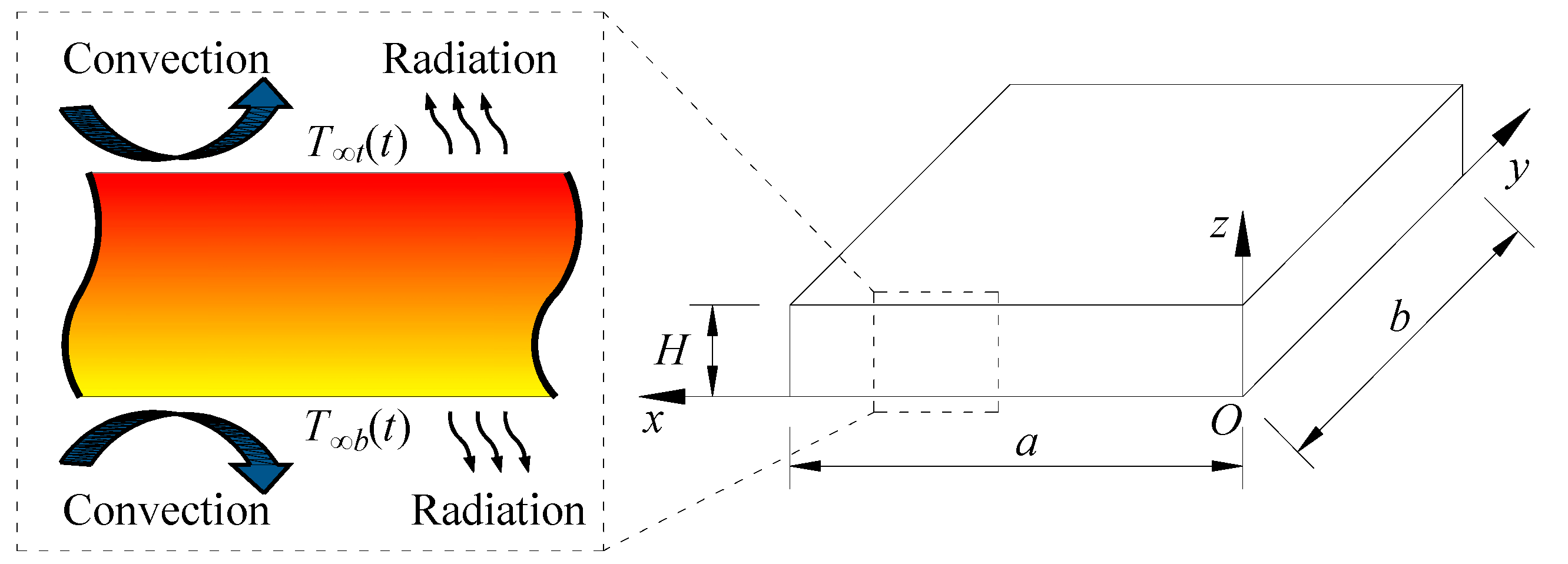
2. Heat Transfer Analysis

Figure 1 shows a simply supported rectangular plate in the Cartesian coordinate ($0\le x\le a$, $0\le y\le b$, and $0\le z\le H$). In the initial stress-free state, the temperature in the plate is uniform and denoted by $T_0$. We assume that the plate is subjected to convection and radiation boundary conditions from the top and bottom surfaces by external heat sources with T-D temperatures $T_{\infty t}(t)$ and $T_{\infty b}(t)$, respectively. For simplicity, we assume that the temperature only varies along the thickness direction.

Before the heat transfer analysis and thermoelastic analysis, some assumptions are established as:

i.

The plate is made of a homogeneous, isotropic, and temperature-independent material;

ii.

The heat convection coefficient and surface emissivity corresponding to the top and bottom surfaces are considered as constants;

iii.

The plate’s deformation falls within the scope of linear elasticity and small strains.

2.1. Linearization of Radiation Condition

The plate is subjected to T-D convection and radiation boundary conditions, in which the general radiation condition is expressed by [19]

$$q=\sigma \epsilon \left(T_w^4-T_{\infty }^4\right)$$

(1)

where q is the heat flux, $T_{\infty }$ is the surrounding temperature, $T_w$ is the temperature at the surface of the plate, σ ($=5.67\times {10}^{-8}{ \mathrm{W}/(\mathrm{m}}^2\mathrm{K})$) is the Stephan–Boltzmann constant, and ε is the surface emissivity.

Owing to the radiation condition, the heat transfer problem becomes nonlinear and is hard to exactly solve. Hence, a linear approximation of the radiation condition is required. Based on Miller and Weaver’s work [19], Equation (1) can be approximated as

$$q\approx 4\sigma \epsilon T_{\infty }^3{T}_w-4\sigma \epsilon T_{\infty }^4$$

(2)

It is noted that the error induced by the approximation is neglectable when $T_{\infty }$ is T-I and $T_w/T_{\infty }>0.75$ [19]. However, the conditions of $T_w$ and $T_{\infty }$ are not satisfied in the present problem, which makes Equation (2) not suitable for the present problem. To solve it, we divide the whole heating process into several time steps [12], each of which is assumed to start from zero, i.e., $t\in [0, \Delta t]$. The convection and radiation conditions on the surfaces of the plate within a time step can be written as [20]

$$-\lambda \frac{\partial T_{wj}}{\partial z}+h_j\left(T_{wj}-T_{\infty j}\right)+\sigma \epsilon T_{wj}^4-\sigma \epsilon {(r_j{T}_{\infty j})}^4+\sigma \epsilon {(r_j{T}_{\infty j})}^4-\sigma \epsilon T_{\infty j}^4=0, j=t \mathrm{or} b, t\in [0, \Delta t]$$

(3)

It should be noted that by taking j = t and j = b in Equation (3), two equations, i.e., the boundary conditions on the top and bottom surfaces, will be generated. λ is the thermal conductivity, h is the heat convection coefficient, and the factor r is given by [20]

$$r_j=\left\{\begin{array}{ll}\frac{T_{wj}\left(t=0\right)}{0.9{\overline{T}}_{\infty j}},& \mathrm{when} \left|{\overline{T}}_{\infty j}-T_{wj}\left(t=0\right)\right|>0.1T_{wj}\left(t=0\right)\\ 1,& \mathrm{when} \left|{\overline{T}}_{\infty j}-T_{wj}\left(t=0\right)\right|\le 0.1T_{wj}\left(t=0\right)\end{array}\right.$$

(4)

where ${\overline{T}}_{\infty j}=0.5[T_{\infty j}(t=0)+T_{\infty j}(t=\Delta t)]$. It is clear that the use of Equation (4) guarantees $T_{wj}/(r_j{\overline{T}}_{\infty j})>0.75$. By applying Equation (2) to Equation (3) and replacing $T_{\infty j}$ with ${\overline{T}}_{\infty j}$ in some terms, Equation (3) can be simplified as

$$-\lambda \frac{\partial T_{wt}}{\partial z}+{\zeta }_t{T}_{wt}={\zeta }_t^{\prime }{T}_{\infty t}, -\lambda \frac{\partial T_{wb}}{\partial z}+{\zeta }_b{T}_{wb}={\zeta }_b^{\prime }{T}_{\infty b}$$

(5)

where ${\zeta }_j=h_j+4\sigma \epsilon {\left(r_j{\overline{T}}_{\infty j}\right)}^3$ and ${\zeta }_j^{\prime }=h_j+\sigma \epsilon {\overline{T}}_{\infty j}^3+3\sigma \epsilon r_j^4{\overline{T}}_{\infty j}^3$ (j = t or b).

2.2. Basic Equations and Homogenization of Boundary Conditions

The transient temperature T(z, t) within a time step is governed by:

i. 1-D transient heat transfer equation [12];

$$\kappa \frac{{\partial }^{2}T(z,t)}{\partial z^2}=\frac{\partial T(z,t)}{\partial t}, t\in [0, \Delta t]$$

(6)

where $\kappa =\lambda /\rho c$ is the thermal diffusivity, ρ is the density, and c is the specific heat.

ii. Simplified convection and radiation conditions on the top and bottom surfaces, as shown in Equation (5);

iii. Initial temperature;

$$T(z,0)\triangleq F(z)$$

(7)

It is found that the present heat transfer problem contains a homogeneous governing equation (Equation (6)) and two non-homogeneous boundary conditions (Equation (5)). To homogenize the boundary conditions, a new variable θ(z, t) is introduced as follows:

$$T(z,t)=\theta (z,t)+q(z,t)$$

(8)

where $q(z,t)=\frac{{\left(H-z\right)}^2{\zeta }_t^{\prime }{T}_{\infty t}\left(t\right)}{H\left({\zeta }_{t}H+2\lambda \right)}+\frac{z^2{\zeta }_b^{\prime }{T}_{\infty b}\left(t\right)}{H\left({\zeta }_{b}H+2\lambda \right)}$.

Applying Equation (8) to Equations (5)–(7) gives

$$\kappa \frac{{\partial }^2\theta (z,t)}{\partial z^2}-\frac{\partial \theta (z,t)}{\partial t}=-\kappa \frac{{\partial }^{2}q(z,t)}{\partial z^2}+\frac{\partial q(z,t)}{\partial t}$$

(9)

$$\lambda \frac{\partial \theta (z,t)}{\partial z}+{\zeta }_t\theta (z,t)=0, \mathrm{at} z=H;$$

$$-\lambda \frac{\partial \theta (z,t)}{\partial x}+{\zeta }_b\theta (z,t)=0, \mathrm{at} z=0$$

(10)

$$\theta (z,0)=F(z)-q(z,0)\triangleq f(z)$$

(11)

It can be seen that the homogenization of the boundary conditions (Equation (10)) yields a non-homogeneous governing equation (Equation (9)).

2.3. Solution of Space-Variable

The corresponding homogeneous equation of Equation (9) can be obtained by setting the right side of Equation (9) as zero, i.e.,

$$\kappa \frac{{\partial }^2\theta (z,t)}{\partial z^2}-\frac{\partial \theta (z,t)}{\partial t}=0$$

(12)

Applying the technique of the separation of variables to θ(z, t) gives

$$\theta (z,t)={\displaystyle \sum _{m=1}^{\infty }{\Phi }_m\left(z\right){\Gamma }_m\left(t\right)}$$

(13)

Substituting Equation (13) into Equation (12) for each term m yields

$$\kappa \frac{\frac{d^2{\Phi }_m(z)}{d{z}^2}}{{\Phi }_m(z)}=\frac{\frac{d{\Gamma }_m(t)}{dt}}{{\Gamma }_m(t)}=-{\beta }_m^2$$

(14)

where ${\beta }_m$ is the separation constant. Using Equation (14) gives the following equation:

$$\kappa \frac{d^2{\Phi }_m(z)}{d{z}^2}+{\beta }_m^2{\Phi }_m(z)=0$$

(15)

where only the space-variable ${\Phi }_m(z)$ is included. The solution of Equation (15) is

$${\Phi }_m(z)=A_m\cos (\frac{{\beta }_{m}z}{\sqrt{\kappa }})+B_m\sin (\frac{{\beta }_{m}z}{\sqrt{\kappa }})$$

(16)

Substituting Equation (16) into Equation (10) gives

$$\mathit{C}{\left\{\begin{array}{cc}{A}_m& B_m\end{array}\right\}}^T=\mathbf{0}$$

(17)

where

$$\mathit{C}=\left[\begin{array}{cc}{\zeta }_t& -\frac{\lambda {\beta }_m}{\sqrt{\kappa }}\\ {\zeta }_b\cos (\frac{{\beta }_{m}H}{\sqrt{\kappa }})-\frac{\lambda {\beta }_m}{\sqrt{\kappa }}\sin (\frac{{\beta }_{m}H}{\sqrt{\kappa }})& {\zeta }_b\sin (\frac{{\beta }_{m}H}{\sqrt{\kappa }})+\frac{\lambda {\beta }_m}{\sqrt{\kappa }}\cos (\frac{{\beta }_{m}H}{\sqrt{\kappa }})\end{array}\right]$$

(18)

According to Cramer’s rule, the non-zero solutions of Equation (17) exist only if the determinant $\left|\mathit{C}\right|=0$. The positive roots of $\left|\mathit{C}\right|=0$ give the eigenvalues ${\beta }_1<{\beta }_2<\dots <{\beta }_m$. Applying each eigenvalue ${\beta }_m$ to Equation (17) obtains $A_m$ and $B_m$, where $A_m$ can be determined arbitrarily. For example, setting $A_m=1$ gives $B_m={\zeta }_t\sqrt{\kappa }/(\lambda {\beta }_m)$.

2.4. Solution of Time-Variable

After finding the complete solution of the space-variable ${\Phi }_m(z)$, we will solve the time-variable ${\Gamma }_m(t)$ in this section. To this end, the right side of Equation (9), $\kappa {\partial }^{2}q(z,t)/\partial z^2$ and $\partial q(z,t)/\partial t$, and the initial condition Equation (11), $f(z)$, should be rewritten in the Fourier series form in terms of ${\Phi }_m(z)$:

$$\kappa \frac{{\partial }^{2}q(z,t)}{\partial z^2}={\displaystyle \sum _{m=1}^{\infty }{I}_m^{\ast }(t){\Phi }_m(z)}, \frac{\partial q(z,t)}{\partial t}={\displaystyle \sum _{m=1}^{\infty }{V}_m^{\ast }(t){\Phi }_m(z)}, f(z)={\displaystyle \sum _{m=1}^{\infty }{f}_m^{\ast }{\Phi }_m(z)}$$

(19)

Based on the orthogonality of ${\Phi }_m(z)$ [16], the unknowns $I_m^{\ast }(t)$, $V_m^{\ast }(t)$, and $f_m^{\ast }$ can be obtained as follows:

$$I_m^{\ast }(t)=\frac{1}{N_m}{\displaystyle {\int }_0^H\kappa \frac{{\partial }^{2}q(z,t)}{\partial z^2}{\Phi }_m(z)dz}, V_m^{\ast }(t)=\frac{1}{N_m}{\displaystyle {\int }_0^H\frac{\partial q(z,t)}{\partial t}{\Phi }_m(z)dz}$$

$$f_m^{\ast }=\frac{1}{N_m}{\displaystyle {\int }_0^{H}f(z){\Phi }_m(z)dz}$$

(20)

where $N_m={\displaystyle {\int }_0^H{[{\Phi }_m(z)]}^{2}dz}$.

Substituting Equations (13) and (19) into Equation (9) and using Equation (15) gives

$$\frac{d{\Gamma }_m(t)}{dt}+{\Gamma }_m(t){\beta }_m^2=I_m^{\ast }(t)-V_m^{\ast }(t)$$

(21)

The initial value ${\Gamma }_m(0)$ must be given to solve Equation (21). Using Equations (11) and (13) gives

$$\theta (z,0)\triangleq f(z)={\displaystyle \sum _{m=1}^{\infty }{\Phi }_m(z){\Gamma }_m(0)}$$

(22)

Comparing the third of Equation (19) and Equation (22) obtains ${\Gamma }_m(0)=f_m^{\ast }$, then the solution of Equation (21) is

$${\Gamma }_m(t)=\exp (-{\beta }_m^{2}t)\left\{{\displaystyle {\int }_0^t\exp ({\beta }_m^2\tau )\left[I_m^{\ast }(\tau )-V_m^{\ast }(\tau )\right]d\tau }+f_m^{\ast }\right\}$$

(23)

Finally, the transient temperature can be obtained using Equations (8), (13), and (23)

$$T(z,t)=q(z,t)+{\displaystyle \sum _{m=1}^{\infty }{\Phi }_m(z)\exp (-{\beta }_m^{2}t)\left\{{\displaystyle {\int }_0^t\exp ({\beta }_m^2\tau )\left[I_m^{\ast }(\tau )-V_m^{\ast }(\tau )\right]d\tau }+f_m^{\ast }\right\}}$$

(24)

2.5. Calculation Procedure of Temperature Solution

The numerical results of the transient temperature can be obtained in four steps as follows:

Step 1: Select an appropriate time interval $\Delta t_i$ ($i\in {\mathit{N}}^{+}$) for each time step. The time interval $\Delta t_i$ should satisfy the condition $\left|T_{\infty }(t_i=0)-T_{\infty }(t_i=\Delta t_i)\right|\le 0.01T_{\infty \max }$, where $T_{\infty \max }$ denotes the maximum surrounding temperature during the whole heating process [9].

Step 2: The initial temperature in the ith time step is equal to the temperature at the end of the (i − 1)th time step, i.e., $F_i(z)=T_{i-1}(z,\Delta t_{i-1})$.

Step 3: The transient temperature $T_i(z,t_i)$ in the ith time step can be obtained based on the method introduced in Section 2.1, Section 2.2, Section 2.3 and Section 2.4.

Step 4: Repeating steps 1–3 obtains the transient temperature $T_{i+1}(z,t_{i+1})$ in the (i + 1)th time step.

3. Thermoelastic Analysis

3.1. Thermoelasticity Equations

The thermoelastic analysis of the plate is within the framework of 3D thermoelasticity theory. Thus, the deformation and stress states are governed by [45,54]:

i. Geometrical relations;

$${\epsilon }_x=\frac{\partial u}{\partial x}, {\epsilon }_y=\frac{\partial v}{\partial y}, {\epsilon }_z=\frac{\partial w}{\partial z}, {\gamma }_{xy}=\frac{\partial u}{\partial y}+\frac{\partial v}{\partial x}, {\gamma }_{xz}=\frac{\partial u}{\partial z}+\frac{\partial w}{\partial x}, {\gamma }_{yz}=\frac{\partial v}{\partial z}+\frac{\partial w}{\partial y}$$

(25)

ii. Equilibrium equations;

$$\frac{\partial {\sigma }_x}{\partial x}+\frac{\partial {\tau }_{xy}}{\partial y}+\frac{\partial {\tau }_{xz}}{\partial z}=0, \frac{\partial {\tau }_{xy}}{\partial x}+\frac{\partial {\sigma }_y}{\partial y}+\frac{\partial {\tau }_{yz}}{\partial z}=0, \frac{\partial {\tau }_{xz}}{\partial x}+\frac{\partial {\tau }_{yz}}{\partial y}+\frac{\partial {\sigma }_z}{\partial z}=0$$

(26)

iii. Thermoelastic constitutive relations;

$$\left\{\begin{array}{c}{\sigma }_x\\ {\sigma }_y\\ {\sigma }_z\\ {\tau }_{yz}\\ {\tau }_{xz}\\ {\tau }_{xy}\end{array}\right\}=\left[\begin{array}{cccccc}\lambda +2G& \lambda & \lambda & 0& 0& 0\\ \lambda & \lambda +2G& \lambda & 0& 0& 0\\ \lambda & \lambda & \lambda +2G& 0& 0& 0\\ 0& 0& 0& G& 0& 0\\ 0& 0& 0& 0& G& 0\\ 0& 0& 0& 0& 0& G\end{array}\right]\left\{\begin{array}{c}{\epsilon }_x\\ {\epsilon }_y\\ {\epsilon }_z\\ {\gamma }_{yz}\\ {\gamma }_{xz}\\ {\gamma }_{xy}\end{array}\right\}-\left\{\begin{array}{c}P\\ P\\ P\\ 0\\ 0\\ 0\end{array}\right\}$$

(27)

iv. Simply supported edge conditions;

$${\left\{\begin{array}{ccc}{\sigma }_x& v& w\end{array}\right\}}_{x=0, a}={\left\{\begin{array}{ccc}{\sigma }_y& u& w\end{array}\right\}}_{y=0, b}=\mathbf{0}$$

(28)

v. Surface stress conditions;

$${\left\{\begin{array}{ccc}{\sigma }_z& {\tau }_{xz}& {\tau }_{yz}\end{array}\right\}}_{z=H}={\left\{\begin{array}{ccc}{\sigma }_z& {\tau }_{xz}& {\tau }_{yz}\end{array}\right\}}_{z=0}=\mathbf{0}$$

(29)

In Equations (25)–(29) $\left\{\begin{array}{cccccc}{\sigma }_x& {\sigma }_y& {\sigma }_z& {\tau }_{xy}& {\tau }_{xz}& {\tau }_{yz}\end{array}\right\}$ are stress components, $\left\{\begin{array}{cccccc}{\epsilon }_x& {\epsilon }_y& {\epsilon }_z& {\gamma }_{xy}& {\gamma }_{xz}& {\gamma }_{yz}\end{array}\right\}$ strain components, $\left\{\begin{array}{ccc}u& v& w\end{array}\right\}$ displacement components, and

$$\lambda =\frac{\mu E}{(1+\mu )(1-2\mu )}, G=\frac{E}{2(1+\mu )}, P(z,t)=(3\lambda +2G)[T(z,t)-T_0]\alpha$$

(30)

where α is the thermal expansion coefficient, E is Young’s modulus, and μ is Poisson’s ratio.

Applying the state-space method [45] to Equations (25)–(27) gives

$$\frac{\partial }{\partial z}\left\{\begin{array}{c}u\\ v\\ {\sigma }_z\\ {\tau }_{xz}\\ {\tau }_{yz}\\ w\end{array}\right\}=\left[\begin{array}{cccccc}0& 0& 0& S_6& 0& -\varphi \\ 0& 0& 0& 0& S_6& -\phi \\ 0& 0& 0& -\varphi & -\phi & 0\\ -(S_2{\varphi }^2+S_4{\phi }^2)& -(S_3+S_4)\varphi \phi & S_1\varphi & 0& 0& 0\\ -(S_3+S_4)\varphi \phi & -(S_4{\varphi }^2+S_2{\phi }^2)& S_1\phi & 0& 0& 0\\ S_1\varphi & S_1\phi & S_5& 0& 0& 0\end{array}\right]\left\{\begin{array}{c}u\\ v\\ {\sigma }_z\\ {\tau }_{xz}\\ {\tau }_{yz}\\ w\end{array}\right\}+\left\{\begin{array}{c}0\\ 0\\ 0\\ (1+S_1)\varphi P\\ (1+S_1)\phi P\\ S_{5}P\end{array}\right\}$$

(31)

where

$$S_1=-\frac{\lambda }{\lambda +2G}, S_2=\frac{4G(\lambda +G)}{\lambda +2G}, S_3=\frac{2\lambda G}{\lambda +2G}, S_4=G, S_5=\frac{1}{\lambda +2G}, S_6=\frac{1}{G}, \varphi =\frac{\partial }{\partial x}, \phi =\frac{\partial }{\partial y}$$

(32)

The stress components ${\sigma }_x$, ${\sigma }_y$, and ${\tau }_{xy}$ can be solved by

$$\left\{\begin{array}{c}{\sigma }_x\\ {\sigma }_y\\ {\tau }_{xy}\end{array}\right\}=\left[\begin{array}{ccc}{S}_2\varphi & S_3\phi & -S_1\\ S_3\varphi & S_2\phi & -S_1\\ S_4\phi & S_4\varphi & 0\end{array}\right]\left\{\begin{array}{c}u\\ v\\ {\sigma }_z\end{array}\right\}-\left\{\begin{array}{c}(1+S_1)P\\ (1+S_1)P\\ 0\end{array}\right\}$$

(33)

3.2. General Displacement and Stress Solutions

Because the plate is simply supported at its four edges, the displacement and stress solutions can be assumed as

$$\left\{\begin{array}{c}u(x,y,z,t)\\ v(x,y,z,t)\\ w(x,y,z,t)\\ {\sigma }_z(x,y,z,t)\\ {\tau }_{xz}(x,y,z,t)\\ {\tau }_{yz}(x,y,z,t)\end{array}\right\}={\displaystyle \sum _{r=1}^{\infty }{\displaystyle \sum _{s=1}^{\infty }\left\{\begin{array}{c}{U}_{r,s}(z,t)\cos (a_{r}x)\sin (b_{s}y)\\ V_{r,s}(z,t)\sin (a_{r}x)\cos (b_{s}y)\\ W_{r,s}(z,t)\sin (a_{r}x)\sin (b_{s}y)\\ Z_{r,s}(z,t)\sin (a_{r}x)\sin (b_{s}y)\\ X_{r,s}(z,t)\cos (a_{r}x)\sin (b_{s}y)\\ Y_{r,s}(z,t)\sin (a_{r}x)\cos (b_{s}y)\end{array}\right\}}}$$

(34)

where $a_r$ = rπ/a and $b_s$ = sπ/b.

Similarly, the thermoelastic term P(z, t) in Equations (31) and (33) can be expanded as

$$P(x,y,z,t)={\displaystyle \sum _{r=1}^{\infty }{\displaystyle \sum _{s=1}^{\infty }{P}_{r,s}(z,t)\sin (a_{r}x)\sin (b_{s}y)}}$$

(35)

where $P_{r,s}(z,t)=\frac{4}{ab}{\displaystyle {\int }_0^a{\displaystyle {\int }_0^{b}P(z,t)\sin (a_{r}x)\sin (b_{s}y)dxdy}}$.

Applying Equations (34) and (35) to Equations (33) gives

$${\sigma }_x(x,y,z,t)=-{\displaystyle \sum _{r=1}^{\infty }{\displaystyle \sum _{s=1}^{\infty }[S_2{a}_r{U}_{r,s}(z,t)+S_3{b}_s{V}_{r,s}(z,t)+S_1{Z}_{r,s}(z,t)}}+(1+S_1)P_{r,s}(z,t)]\sin (a_{r}x)\sin (b_{s}y),$$

$${\sigma }_y(x,y,z,t)=-{\displaystyle \sum _{r=1}^{\infty }{\displaystyle \sum _{s=1}^{\infty }[S_3{a}_r{U}_{r,s}(z,t)+S_2{b}_s{V}_{r,s}(z,t)+S_1{Z}_{r,s}(z,t)}}+(1+S_1)P_{r,s}(z,t)]\sin (a_{r}x)\sin (b_{s}y),$$

$${\tau }_{xy}(x,y,z,t)={\displaystyle \sum _{r=1}^{\infty }{\displaystyle \sum _{s=1}^{\infty }[S_4{b}_s{U}_{r,s}(z,t)+S_4{a}_r{V}_{r,s}(z,t)]\cos (a_{r}x)\cos (b_{s}y)}}$$

(36)

According to Equations (34) and (36), we can find that the edge conditions (see Equation (28)) are satisfied.

Applying Equations (34) and (35) to Equation (31) gives

$$\frac{\partial \mathit{P}(z,t)}{\partial z}=\mathit{A}\mathit{P}(z,t)+\mathit{B}(z,t)$$

(37)

where

$$\mathit{P}(z,t)=\left\{\begin{array}{c}{U}_{r,s}(z,t)\\ V_{r,s}(z,t)\\ Z_{r,s}(z,t)\\ X_{r,s}(z,t)\\ Y_{r,s}(z,t)\\ W_{r,s}(z,t)\end{array}\right\}, \mathit{B}(z,t)=\left\{\begin{array}{c}0\\ 0\\ 0\\ (1+S_1)a_r{P}_{r,s}(z,t)\\ (1+S_1)b_s{P}_{r,s}(z,t)\\ S_5{P}_{r,s}(z,t)\end{array}\right\},$$

$$\mathit{A}=\left[\begin{array}{cccccc}0& 0& 0& S_6& 0& -a_r\\ 0& 0& 0& 0& S_6& -b_s\\ 0& 0& 0& a_r& b_s& 0\\ S_2{a}_r^2+S_4^i{b}_s^2& (S_3+S_4)a_r{b}_s& S_1{a}_r& 0& 0& 0\\ (S_3+S_4)a_r{b}_s& S_4{a}_r^2+S_2{b}_s^2& S_1{b}_s& 0& 0& 0\\ -S_1{a}_r& -S_1{b}_s& S_5& 0& 0& 0\end{array}\right]$$

(38)

Based on the matrix theory, the solution to Equation (37) is [45]

$$\mathit{P}(z,t)=\mathit{M}(z)\mathit{P}(0,t)+\mathit{N}(z,t)$$

(39)

where $\mathit{M}(z)=\exp (\mathit{A}z)$ and $\mathit{N}(z,t)={\displaystyle {\int }_0^z\exp [\mathit{A}(z-\tau )]\mathit{B}(\tau ,t)d\tau }$. To calculate $\mathit{M}(z)$ and $\mathit{N}(z,t)$, the eigenvalues of A should be taken into consideration. Let ${\kappa }_i$ (i = 1, 2, …, 6) be the eigenvalues of A and ${\mathit{J}}_i$ (i = 1, 2, …, 6) be the corresponding eigenvectors, then there must exist a matrix $\mathit{K}=[\begin{array}{cccc}{\mathit{J}}_1& {\mathit{J}}_2& \cdots & {\mathit{J}}_6\end{array}]$ and its inverse matrix ${\mathit{K}}^{-1}$ which can transform A into a diagonal matrix. In this case, we have

$$\mathit{M}(z)=\exp (\mathit{A}z)=\mathit{K}\left[\begin{array}{ccc}\exp ({\kappa }_{1}z)& & 0\\ & \ddots & \\ 0& & \exp ({\kappa }_{6}z)\end{array}\right]{\mathit{K}}^{-1}$$

(40)

Therefore

$$\mathit{N}(z,t)={\displaystyle {\int }_0^z\mathit{K}\left[\begin{array}{ccc}\exp [{\kappa }_1(z-\tau )]& & 0\\ & \ddots & \\ 0& & \exp [{\kappa }_6(z-\tau )]\end{array}\right]{\mathit{K}}^{-1}\mathit{B}(\tau ,t)d\tau }$$

(41)

3.3. Determination of Unknowns

By applying Equations (34) and (35) to Equation (29), the surface stress conditions can be rewritten as

$$\mathit{P}(H,t)=\left\{\begin{array}{cccccc}{U}_{r,s}(H,t)& V_{r,s}(H,t)& 0& 0& 0& W_{r,s}(H,t)\end{array}\right\},$$

(42)

$$\mathit{P}(0,t)=\left\{\begin{array}{cccccc}{U}_{r,s}(0,t)& V_{r,s}(0,t)& 0& 0& 0& W_{r,s}(0,t)\end{array}\right\}$$

(43)

Taking z = H into Equation (39) yields

$$\mathit{P}(H,t)=\mathit{M}(H)\mathit{P}(0,t)+\mathit{N}(H,t)$$

(44)

After eliminating $U_{r,s}(H,t)$, $V_{r,s}(H,t)$, and $W_{r,s}(H,t)$ from Equation (44), we have

$$\left\{\begin{array}{c}{U}_{r,s}(0,t)\\ V_{r,s}(0,t)\\ W_{r,s}(0,t)\end{array}\right\}=-{\left[\begin{array}{ccc}{M}_{31}& M_{32}& M_{36}\\ M_{41}& M_{42}& M_{46}\\ M_{51}& M_{52}& M_{56}\end{array}\right]}^{-1}\left\{\begin{array}{c}{N}_3\\ N_4\\ N_5\end{array}\right\}$$

(45)

where $M_{ij}$ is the element of the matrix M(H) and $N_i$ is the element of the vector N(H, t). Calculating Equation (45) gives P(0, t), and applying P(0, t) to Equation (39) gives P(z, t). Finally, the displacement and stress solutions are obtained from Equations (34) and (36).

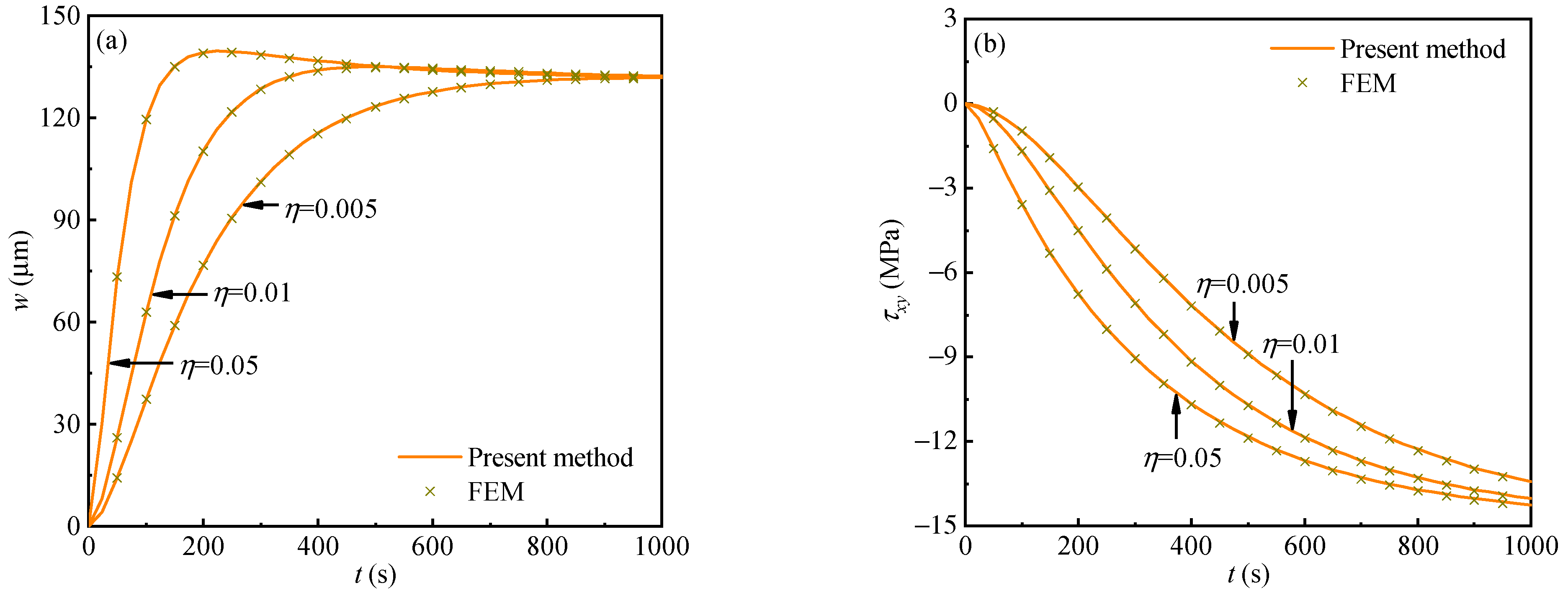
4. Numerical Results and Discussion

In the following numerical calculation, the first 40 eigenvalues (i.e., ${\beta }_1$, ${\beta }_2$, …, ${\beta }_{40}$) are used to obtain the temperature solution, and the first 25 × 25 terms (i.e., r = s = 1, 2, …, 25) are used to obtain the displacement and stress solutions.

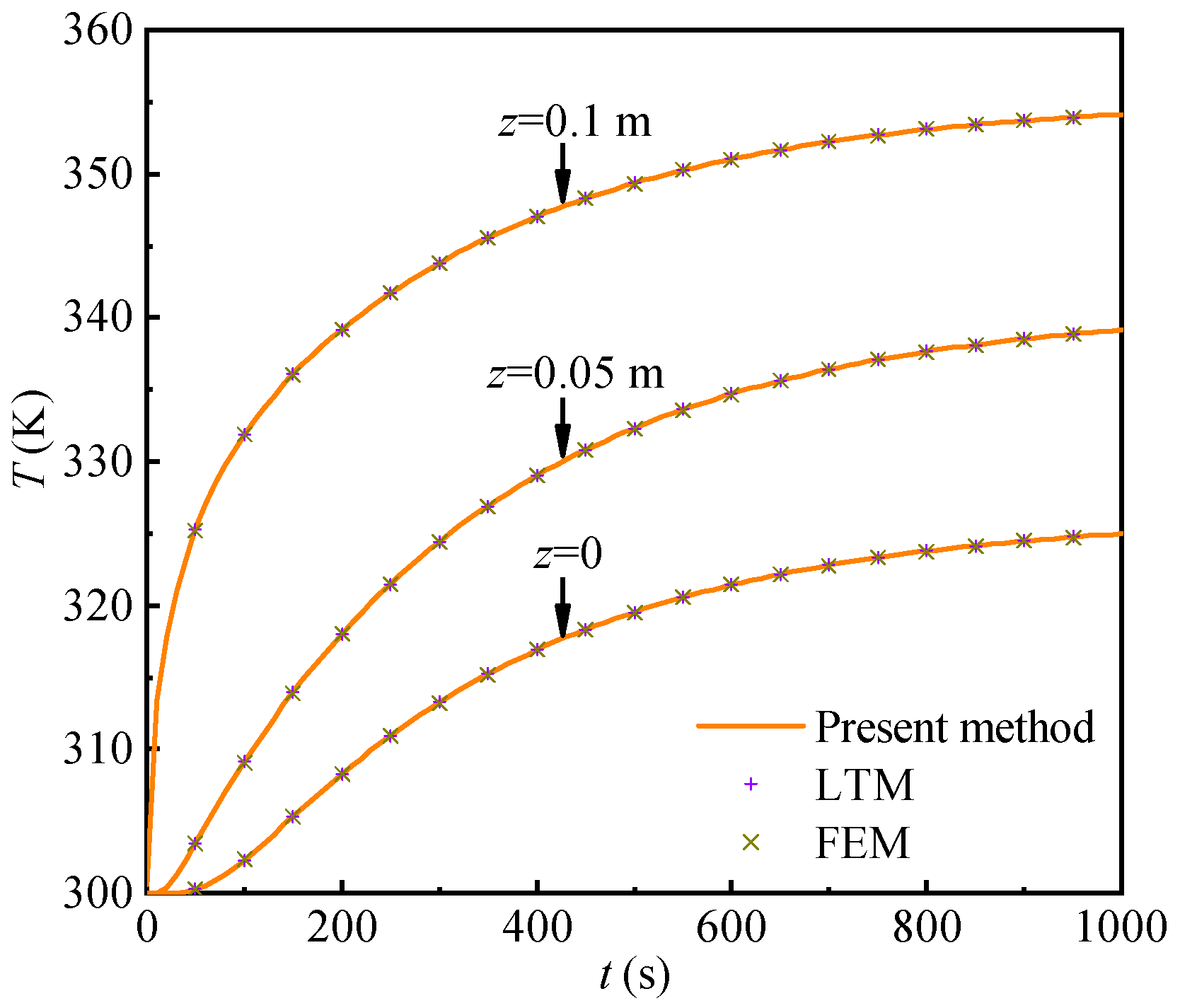
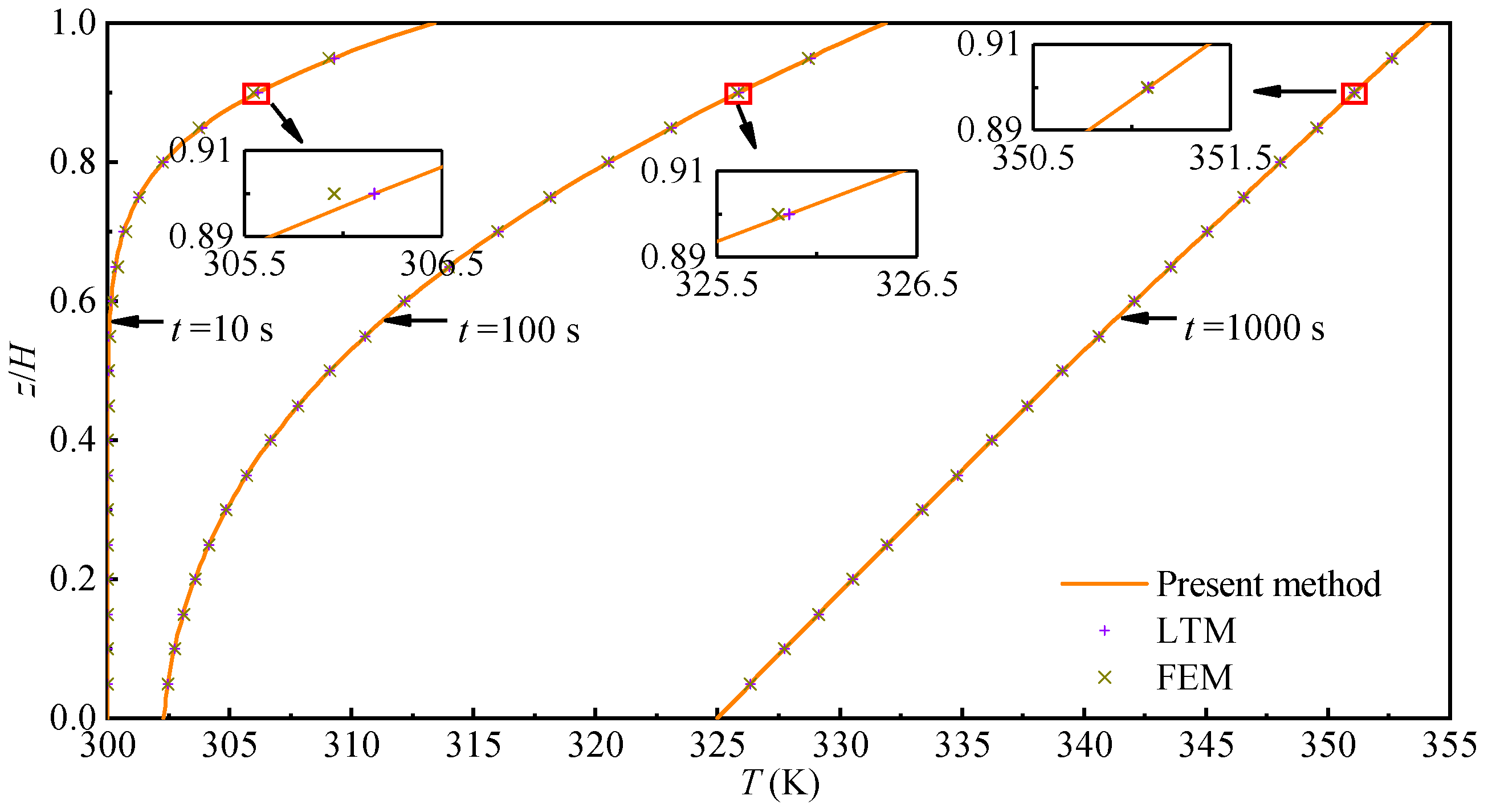
4.1. Validation Study

As no published results for the rectangular plates under current consideration are available in the open literature, two examples concerning the transient heat transfer and thermal bending behaviors are used to validate the present methods by comparing our results with the published ones.

First, the comparison of the transient heat transfer behavior is carried out. Monds and McDonald [55] built two mathematical models, namely, the finite-length scale model and semi-infinite model, to estimate the 1-D transient temperature in human skin during a simulated fire. The accuracy of the models was checked by comparison with the experimental results. In their work, the material properties and thickness of the skin simulant are the following: $\lambda =0.97 \mathrm{W}/(\mathrm{m}\cdot °\mathrm{C})$, $\rho =1877{ \mathrm{kg}/\mathrm{m}}^3$, $c=1205 \mathrm{J}/(\mathrm{kg}\cdot °\mathrm{C})$, and H = 19.66 mm. The temperatures at the top and bottom surfaces of the skin simulant are the following: $T_t=0.0013t^2-0.0696t+21.757 °\mathrm{C}$ and $T_b=-0.0093t^2+2.1531t+60.255 °\mathrm{C}$. Here, we use the present method to estimate the temperature variations at z = 11.12 mm and compare our results with the published ones [55]. The comparative results are shown in Figure 2. The present results match well with those of the finite-length scale model, but have a slight difference from the experimental ones when t > 100 s. The results of the semi-infinite model are more inaccurate compared with the present method and the finite-length scale model.

Then, the comparison of the thermal bending behavior is carried out. Fogang [56] provided the thermal bending analysis of a rectangular plate under linear temperature distribution across the thickness. Here, we use the present method to estimate the central deflection of the plate, and compare our results with the published ones [56]. The deflection is expressed in the following nondimensional form:

$$\overline{w}=\frac{H}{b^2\alpha (\Delta T_t-\Delta T_b)}w$$

(46)

where $\Delta T_t$ and $\Delta T_b$ are the temperature increments at the top and bottom surfaces of the plate, respectively.

Table 1. Central deflection for different aspect ratios a/b and different Poisson’s ratios.

Poisson’s Ratio	Aspect Ratio	Fogang [56]	Present	Error (%)
μ = 0	a/b = 1	0.0737	0.0734	0.41
	a/b = 1.5	0.1008	0.1005	0.30
	a/b = 2	0.1139	0.1136	0.26
	a/b = 3	0.1227	0.1224	0.24
	a/b = 5	0.1249	0.1247	0.16
	a/b = 10	0.1250	0.1251	0.08
μ = 0.2	a/b = 1	0.0884	0.0881	0.34
	a/b = 1.5	0.1209	0.1206	0.25
	a/b = 2	0.1366	0.1363	0.22
	a/b = 3	0.1472	0.1469	0.20
	a/b = 5	0.1499	0.1497	0.13
	a/b = 10	0.1500	0.1501	0.07

shows the comparative results for different aspect ratios a/b and different Poisson’s ratios. The present results match well with those reported by Fogang [56]. The maximum error is less than 0.5%.

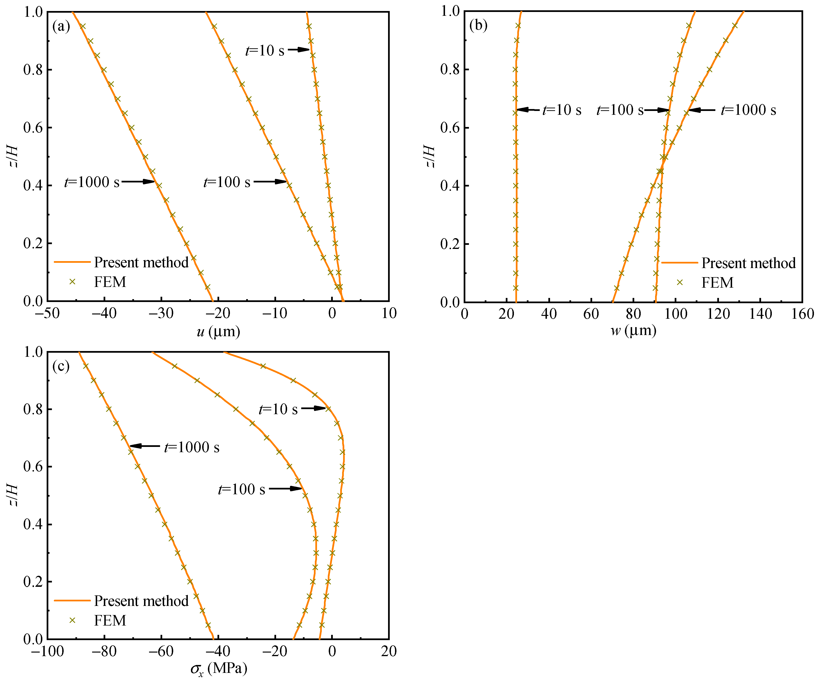
4.2. Purely Convection Boundary and T-I Surrounding Temperature

Consider a rectangular steel plate with the sizes given by the following: a = 0.8 m, b = 0.6 m, and H = 0.1 m. The material properties of the plate are as follows [45]: $\lambda =54.33 \mathrm{W}/(\mathrm{m}\cdot \mathrm{K})$, $\rho =7850{ \mathrm{kg}/\mathrm{m}}^3$, $c=440 \mathrm{J}/(\mathrm{kg}\cdot \mathrm{K})$, ε = 0.7, E = 210 GPa, μ = 0.3, and $\alpha =1.216\times {10}^{-5}{ \mathrm{K}}^{-1}$. The initial temperature is fixed at $T_0=300 \mathrm{K}$. The heat convection coefficients of the top and bottom surfaces are $h_t=800{ \mathrm{W}/(\mathrm{m}}^2\cdot \mathrm{K})$ and $h_b=600{ \mathrm{W}/(\mathrm{m}}^2\cdot \mathrm{K})$, respectively. The bottom surrounding temperature is T-I and fixed at $T_{\infty b}=300 \mathrm{K}$, while the top surrounding temperature $T_{\infty t}$ is variable.

Consider that the plate is subjected to purely convection boundary conditions. The top surrounding temperature is T-I and fixed at $T_{\infty t}=375 \mathrm{K}$. Owing to the omission of the radiation boundary, the whole heating process need not be divided into several time steps. A 3-D FEM analysis is carried out for comparison by use of the software ABAQUS. The transient heat transfer and thermoelastic behaviors are simulated by using the 8-node element DC3D8 and C3D8R, respectively, and by meshing the plate with 80, 60, and 20 elements in the x-, y-, and z-directions, respectively.

Figure 3 shows the comparative results among the time history of the temperature obtained from the present method, the FEM, and the LTM [11] at z = 0, z = 0.05 m, and z = 0.1 m. A good agreement can be found among the three methods. The temperature changes quickly in the early stage and tends to be stable after about t = 900 s. It is also noticed that the higher the position is, the earlier the temperature starts to rise. This is because the heat flows from the top surface (z = 0.1 m) to the bottom surface (z = 0).

Figure 4 shows the comparative results among the temperature distributions obtained from the present method, the FEM, and the LTM [11] at t = 10 s, t = 100 s, and t = 1000 s. It is noticed that the accuracy of the FEM solution improves with time, since the FEM simulation cannot provide a highly accurate prediction when the temperature changes quickly at the early stage. It is also seen that the temperature distribution progressively changes from nonlinearity to linearity with time. This is because of the homogeneity and temperature independency of the material properties, resulting in linear heat conduction in the equilibrium stage.

Figure 5 shows the through-thickness distributions of u, w, and ${\sigma }_x$ at x = 0.2 m, y = 0.15 m for different times t = 10 s, t = 100 s, and t = 1000 s. It is seen that the displacement and stress distributions obtained from the present method and the FEM have a good agreement. Figure 5a–c show that the deformations and stresses are increased with time because the thermal load is increased with time. The displacements u and w vary slightly with the coordinate z at t = 10 s compared with those at t = 1000 s. Figure 5c shows that the distribution of ${\sigma }_x$ changes from nonlinearity to linearity with time, which is similar to the variation of the temperature distribution.

4.3. Convection and Radiation Boundaries and T-D Surrounding Temperature

Consider that the plate is subjected to convection and radiation boundary conditions. The top surrounding temperature is T-D and expressed as

$$T_{\infty t}=T_0+100[1-\exp (-\eta t)]$$

(47)

where the coefficient η represents the rate of temperature variation. Figure 6 shows the time history of $T_{\infty t}$ for different coefficients η = 0.005, η = 0.01, and η = 0.05. In the following analysis, the interval of each time step is uniform and is taken as $\Delta t_i=2 \mathrm{s}$.

Figure 7 shows the time history of temperature at z = 0 and z = 0.1 m for different coefficients η = 0.005, η = 0.01, and η = 0.05. It can be seen that the present results using $\Delta t_i=2 \mathrm{s}$ match well with the FEM ones. The temperature rises faster with η, since the top surrounding temperature $T_{\infty t}$ rises faster with η (see Figure 6).

Figure 8 shows the temperature distributions at t = 100 s and t = 1000 s for different coefficients η = 0.005, η = 0.01, and η = 0.05. It is seen from Figure 8a,b that the temperature distributions are nonlinear at t = 100 s, but are nearly linear at t = 1000 s, which indicates that the temperature in the plate tends to be stable at about t = 1000 s. It is also noticed that, at t = 100 s, the FEM solution is less accurate with the increase in η; however, a similar phenomenon does not occur at t = 1000 s. This is because the temperature in the plate rises faster with η at the early stage, and tends to be stable at about t = 1000 s.

Figure 9 shows the through-thickness distributions of w and ${\tau }_{xy}$ at x = 0.48 m, y = 0.48 m, and t = 100 s for different coefficients η = 0.005, η = 0.01, and η = 0.05. Figure 9a,b indicate that the maximum absolute values of w and ${\tau }_{xy}$ are increased with η. The slopes of the curves of w and ${\tau }_{xy}$ are both increased with η since the temperature gradient is increased with η (see Figure 8a). It is also noticed from Figure 9a that w is variable with the coordinate z. This demonstrates that the approximate 2-D plate theories, which assume that w is invariable through the thickness direction, may generate errors when estimating the thermomechanical responses of the plate.

Figure 10 shows the time history of w and ${\tau }_{xy}$ at x = 0.48 m, y = 0.48 m, and z = 0.05 m for different coefficients η = 0.005, η = 0.01, and η = 0.05. It is seen that w and ${\tau }_{xy}$ increase quickly with η. It is also found that w increases quickly and tends to be stable after about t = 900 s; however, ${\tau }_{xy}$ still has an obvious increase at t = 1000 s. Figure 10a indicates that the long-term deformations (i.e., deformations at t→∞) of the plate do not vary with η.

To show the effects of radiation heat transfer on the mechanical performance of the plate, two kinds of thermal boundaries are considered: (i) purely convection boundary and (ii) convection and radiation boundaries. Figure 11 shows the through-thickness distributions of w and ${\tau }_{xy}$ at x = 0.48 m, y = 0.48 m, and t = 1000 s for η = 0.01. It is noted that to reduce convection effects, the heat convection coefficients of the top and bottom surfaces are taken as $h_t=h_b=10{ \mathrm{W}/(\mathrm{m}}^2\cdot \mathrm{K})$. It is seen that distributions of w and ${\tau }_{xy}$ are greatly affected by radiation heat transfer. The values of w and ${\tau }_{xy}$ with radiation effects are larger than those without radiation effects because radiation heat transfer will generate a larger thermal load.

5. Conclusions

This work presents approximate analytical solutions for the transient thermoelastic problem of rectangular plates with T-D convection and radiation boundaries. By using a linearized approximation to simplify the radiation term, 1-D temperature distribution is obtained. The displacement and stress distributions are obtained based on the exact 3-D thermoelasticity theory. In the numerical examples, the temperature, displacement, and stress fields in a rectangular plate are studied considering two kinds of thermal boundaries. It is concluded that:

i.

The comparison with the reported results and the FEM results indicates that the present method can give a satisfactory prediction for the thermoelastic responses in the plate.

ii.

The temperature, displacements, and stresses increase quickly in the early stage but tend to eventually stabilize.

iii.

The temperature distribution progressively changes from nonlinearity to linearity with time.

iv.

The temperature, displacements, and stresses increase quickly with the increase in the temperature coefficient η. However, the long-term deformations of the plate do not vary with η.

v.

The radiation heat transfer has a significant effect on the displacement and stress distributions.

References

1. Yan, X.; Lin, C.; Liu, X.; Zheng, T.; Shi, S.; Mao, H. Numerical and Analytical Investigations of the Impact Resistance of Partially Precast Concrete Beams Strengthened with Bonded Steel Plates. Buildings 2023, 13, 696. [Google Scholar] [CrossRef]
2. Jiang, L.; Cheng, R.; Zhang, H.; Ma, K. Human-Induced-Vibration Response Analysis and Comfort Evaluation Method of Large-Span Steel Vierendeel Sandwich Plate. Buildings 2022, 12, 1228. [Google Scholar] [CrossRef]
3. Xie, H.; Shen, C.; Fang, H.; Han, J.; Cai, W. Flexural property evaluation of web reinforced GFRP-PET foam sandwich panel: Experimental study and numerical simulation. Compos. Part B Eng. 2022, 234, 109725. [Google Scholar] [CrossRef]
4. Chen, J.; Zhu, L.; Fang, H.; Han, J.; Huo, R.; Wu, P. Study on the low-velocity impact response of foam-filled multi-cavity composite panels. Thin-Walled Struct. 2022, 173, 108953. [Google Scholar] [CrossRef]
5. Manthena, V.R.; Srinivas, V.B.; Kedar, G.D. Analytical solution of heat conduction of a multilayered annular disk and associated thermal deflection and thermal stresses. J. Therm. Stress. 2020, 43, 563–578. [Google Scholar] [CrossRef]
6. Chen, Y.; Zhang, L.; He, C.; He, R.; Xu, B.; Li, Y. Thermal insulation performance and heat transfer mechanism of C/SiC corrugated lattice core sandwich panel. Aerosp. Sci. Technol. 2021, 111, 106539. [Google Scholar] [CrossRef]
7. Ren, Y.; Huo, R.; Zhou, D. Buckling and post-buckling analysis of restrained non-uniform columns in fire. Eng. Struct. 2022, 272, 114947. [Google Scholar] [CrossRef]
8. Ren, Y.; Huo, R.; Zhou, D. Buckling analysis of non-uniform Timoshenko columns under localised fire. Structures 2023, 51, 1245–1256. [Google Scholar] [CrossRef]
9. Özişik, M.N. Heat Conduction, 2nd ed.; Wiley: New York, NY, USA, 1993. [Google Scholar]
10. Frankel, J.I.; Vick, B. An exact methodology for solving nonlinear diffusion equations based on integral transforms. Appl. Numer. Math. 1987, 3, 467–477. [Google Scholar] [CrossRef]
11. Manthena, V.R.; Kedar, G.D. On thermoelastic problem of a thermosensitive functionally graded rectangular plate with instantaneous point heat source. J. Therm. Stress. 2019, 42, 849–862. [Google Scholar] [CrossRef]
12. Ferraiuolo, M.; Manca, O. Heat transfer in a multi-layered thermal protection system under aerodynamic heating. Int. J. Therm. Sci. 2012, 53, 56–70. [Google Scholar] [CrossRef]
13. Hefni, M.A.; Xu, M.; Zueter, A.F.; Hassani, F.; Eltaher, M.A.; Ahmed, H.M.; Saleem, H.A.; Ahmed, H.A.M.; Hassan, G.S.A.; Ahmed, K.I.; et al. A 3D space-marching analytical model for geothermal borehole systems with multiple heat exchangers. Appl. Therm. Eng. 2022, 216, 119027. [Google Scholar] [CrossRef]
14. Tanigawa, Y.; Murakami, H.; Ootao, Y. Transient thermal stress analysis of a laminated composite beam. J. Therm. Stress. 1989, 12, 25–39. [Google Scholar] [CrossRef]
15. Zhang, Z.; Zhou, D.; Zhang, J.; Fang, H.; Han, H. Transient analysis of layered beams subjected to steady heat supply and mechanical load. Steel Compos. Struct. 2021, 40, 87–100. [Google Scholar] [CrossRef]
16. Yang, W.; Pourasghar, A.; Cui, Y.; Wang, L.; Chen, Z. Transient heat transfer analysis of a cracked strip irradiated by ultrafast Gaussian laser beam using dual-phase-lag theory. Int. J. Heat Mass Transf. 2023, 203, 123771. [Google Scholar] [CrossRef]
17. de Monte, F. Transient heat conduction in one-dimensional composite slab. A ‘natural’ analytic approach. Int. J. Heat Mass Transf. 2000, 43, 3607–3619. [Google Scholar] [CrossRef]
18. de Monte, F. An analytic approach to the unsteady heat conduction processes in one-dimensional composite media. Int. J. Heat Mass Transf. 2002, 45, 1333–1343. [Google Scholar] [CrossRef]
19. Miller, J.R.; Weaver, P.M. Temperature profiles in composite plates subject to time-dependent complex boundary conditions. Compos. Struct. 2003, 59, 267–278. [Google Scholar] [CrossRef]
20. Gu, L.; Wang, Y.; Shi, S.; Dai, C. An approximate analytical method for nonlinear transient heat transfer through a metallic thermal protection system. Int. J. Heat Mass Transf. 2016, 103, 582–593. [Google Scholar] [CrossRef]
21. Reddy, J.N. Mechanics of Laminated Composite Plates and Shells; CRC Press: Boca Raton, FL, USA, 2004. [Google Scholar]
22. Abrate, S.; Di Sciuva, M. Equivalent single layer theories for composite and sandwich structures: A review. Compos. Struct. 2017, 179, 482–494. [Google Scholar] [CrossRef]
23. Tauchert, T.R. Thermally induced flexure, buckling, and vibration of plates. Appl. Mech. Rev. 1991, 44, 347–360. [Google Scholar] [CrossRef]
24. Kulkarni, P.; Dhoble, A.; Padole, P. A review of research and recent trends in analysis of composite plates. Sādhanā 2018, 43, 96. [Google Scholar] [CrossRef]
25. Yang, K.J.; Kang, K.J.; Beom, H.G. Thermal Stress Analysis for an Inclusion with Nonuniform Temperature Distribution in an Infinite Kirchhoff Plate. J. Therm. Stress. 2005, 28, 1123–1144. [Google Scholar] [CrossRef]
26. Ren, Y.; Huo, R.; Zhou, D. Thermo-mechanical buckling analysis of non-uniformly heated rectangular plates with temperature-dependent material properties. Thin-Walled Struct. 2023, 186, 110653. [Google Scholar] [CrossRef]
27. Prakash, A.; Kumar, P.; Saran, V.H.; Harsha, S.P. NURBS based thermoelastic behaviour of thin functionally graded sigmoidal (TFGS) porous plate resting on variable Winkler’s foundation. Int. J. Mech. Mater. Des. 2023. [Google Scholar] [CrossRef]
28. Thongchom, C.; Jearsiripongkul, T.; Refahati, N.; Roudgar Saffari, P.; Roodgar Saffari, P.; Sirimontree, S.; Keawsawasvong, S. Sound Transmission Loss of a Honeycomb Sandwich Cylindrical Shell with Functionally Graded Porous Layers. Buildings 2022, 12, 151. [Google Scholar] [CrossRef]
29. Van Vinh, P.; Van Chinh, N.; Tounsi, A. Static bending and buckling analysis of bi-directional functionally graded porous plates using an improved first-order shear deformation theory and FEM. Eur. J. Mech.-A/Solids 2022, 96, 104743. [Google Scholar] [CrossRef]
30. Qolipour, A.M.; Eipakchi, H.; Nasrekani, F.M. Asymmetric/Axisymmetric buckling of circular/annular plates under radial load using first-order shear deformation theory. Thin-Walled Struct. 2023, 182, 110244. [Google Scholar] [CrossRef]
31. Hauck, B.; Szekrényes, A. Fracture mechanical finite element analysis for delaminated composite plates applying the first-order shear deformation plate theory. Compos. Struct. 2023, 308, 116719. [Google Scholar] [CrossRef]
32. Mei, Y.; Ban, H.; Shi, Y. Elastic buckling of simply supported bimetallic steel plates. J. Constr. Steel Res. 2022, 198, 107581. [Google Scholar] [CrossRef]
33. Roodgar Saffari, P.; Sher, W.; Thongchom, C. Size Dependent Buckling Analysis of a FG-CNTRC Microplate of Variable Thickness under Non-Uniform Biaxial Compression. Buildings 2022, 12, 2238. [Google Scholar] [CrossRef]
34. Van Do, V.N.; Lee, C.-H. Nonlinear thermal buckling analyses of functionally graded circular plates using higher-order shear deformation theory with a new transverse shear function and an enhanced mesh-free method. Acta Mech. 2018, 229, 3787–3811. [Google Scholar] [CrossRef]
35. Moayeri, M.; Darabi, B.; Sianaki, A.H.; Adamian, A. Third order nonlinear vibration of viscoelastic circular microplate based on softening and hardening nonlinear viscoelastic foundation under thermal loading. Eur. J. Mech.-A/Solids 2022, 95, 104644. [Google Scholar] [CrossRef]
36. Vu, N.A.; Pham, T.D.; Tran, T.T.; Pham, Q.-H. Third-order isogeometric analysis for vibration characteristics of FGP plates in the thermal environment supported by Kerr foundation. Case Stud. Therm. Eng. 2023, 45, 102890. [Google Scholar] [CrossRef]
37. Van Do, T.; Hong Doan, D.; Chi Tho, N.; Dinh Duc, N. Thermal Buckling Analysis of Cracked Functionally Graded Plates. Int. J. Struct. Stab. Dyn. 2022, 22, 22500894. [Google Scholar] [CrossRef]
38. Zenkour, A.M.; Alghamdi, N.A. Bending Analysis of Functionally Graded Sandwich Plates under the Effect of Mechanical and Thermal Loads. Mech. Adv. Mater. Struct. 2010, 17, 419–432. [Google Scholar] [CrossRef]
39. Sah, S.K.; Ghosh, A. Effect of Porosity on the Thermal Buckling Analysis of Power and Sigmoid Law Functionally Graded Material Sandwich Plates Based on Sinusoidal Shear Deformation Theory. Int. J. Struct. Stab. Dyn. 2022, 22, 22500638. [Google Scholar] [CrossRef]
40. Bouiadjra, R.B.; Bedia, E.A.A.; Tounsi, A. Nonlinear thermal buckling behavior of functionally graded plates using an efficient sinusoidal shear deformation theory. Struct. Eng. Mech. 2013, 48, 547–567. [Google Scholar] [CrossRef]
41. Houari, M.S.A.; Tounsi, A.; Bessaim, A.; Mahmoud, S.R. A new simple three-unknown sinusoidal shear deformation theory for functionally graded plates. Steel Compos. Struct. 2016, 22, 257–276. [Google Scholar] [CrossRef]
42. Bouazza, M.; Lairedj, A.; Benseddiq, N.; Khalki, S. A refined hyperbolic shear deformation theory for thermal buckling analysis of cross-ply laminated plates. Mech. Res. Commun. 2016, 73, 117–126. [Google Scholar] [CrossRef]
43. Laoufi, I.; Ameur, M.; Zidi, M.; Bedia, E.A.A.; Bousahla, A.A. Mechanical and hygrothermal behaviour of functionally graded plates using a hyperbolic shear deformation theory. Steel Compos. Struct. 2016, 20, 889–911. [Google Scholar] [CrossRef]
44. Benahmed, A.; Houari, M.S.A.; Benyoucef, S.; Belakhdar, K.; Tounsi, A. A novel quasi-3D hyperbolic shear deformation theory for functionally graded thick rectangular plates on elastic foundation. Geomech. Eng. 2017, 12, 9–34. [Google Scholar] [CrossRef]
45. Zhang, Z.; Zhou, D.; Fang, H.; Zhang, J.; Li, X. Analysis of layered rectangular plates under thermo-mechanical loads considering temperature-dependent material properties. Appl. Math. Model. 2021, 92, 244–260. [Google Scholar] [CrossRef]
46. Wang, J.; Yuan, W.; Li, Z.; Trofimov, Y.; Lishik, S.; Fan, J. A neural network-assisted 3D theoretical thermoelastic solution for laminated liquid crystal elastomer plate used in restoring cardiac mechanical function. J. Mech. Behav. Biomed. Mater. 2022, 136, 105478. [Google Scholar] [CrossRef]
47. Aljadani, M.H.; Zenkour, A.M. A Modified Two-Relaxation Thermoelastic Model for a Thermal Shock of Rotating Infinite Medium. Materials 2022, 15, 9056. [Google Scholar] [CrossRef] [PubMed]
48. Zakaria, K.; Sirwah, M.A.; Abouelregal, A.E.; Rashid, A.F. Photo-Thermoelastic Model with Time-Fractional of Higher Order and Phase Lags for a Semiconductor Rotating Materials. Silicon 2021, 13, 573–585. [Google Scholar] [CrossRef]
49. Abouelregal, A.E. Two-temperature thermoelastic model without energy dissipation including higher order time-derivatives and two phase-lags. Mater. Res. Express 2019, 6, 116535. [Google Scholar] [CrossRef]
50. Askar, S.; Abouelregal, A.E.; Marin, M.; Foul, A. Photo-Thermoelasticity Heat Transfer Modeling with Fractional Differential Actuators for Stimulated Nano-Semiconductor Media. Symmetry 2023, 15, 656. [Google Scholar] [CrossRef]
51. Abouelregal, A.E.; Askar, S.S.; Marin, M.; Mohamed, B. The theory of thermoelasticity with a memory-dependent dynamic response for a thermo-piezoelectric functionally graded rotating rod. Sci. Rep. 2023, 13, 9052. [Google Scholar] [CrossRef]
52. Abouelregal, A.E.; Moustapha, M.V.; Nofal, T.A.; Rashid, S.; Ahmad, H. Generalized thermoelasticity based on higher-order memory-dependent derivative with time delay. Results Phys. 2021, 20, 103705. [Google Scholar] [CrossRef]
53. Abouelregal, A.E.; Alesemi, M. Evaluation of the thermal and mechanical waves in anisotropic fiber-reinforced magnetic viscoelastic solid with temperature-dependent properties using the MGT thermoelastic model. Case Stud. Therm. Eng. 2022, 36, 102187. [Google Scholar] [CrossRef]
54. Ying, J.; Lü, C.; Lim, C.W. 3D thermoelasticity solutions for functionally graded thick plates. J. Zhejiang Univ. A 2009, 10, 327–336. [Google Scholar] [CrossRef]
55. Monds, J.R.; McDonald, A.G. Determination of skin temperature distribution and heat flux during simulated fires using Green’s functions over finite-length scales. Appl. Therm. Eng. 2013, 50, 593–603. [Google Scholar] [CrossRef]
56. Fogang, V. Bending Analysis of Isotropic Rectangular Kirchhoff Plates Subjected to Non-Uniform Heating Using the Fourier Transform Method. Preprints 2021, 2021060479. [Google Scholar] [CrossRef]
Figure 1. A rectangular plate with T-D convection and radiation boundaries.
Buildings 13 02174 g001
Figure 2. Time history of temperature at z = 11.12 mm [55].
Buildings 13 02174 g002
Figure 3. Time history of temperature at z = 0, z = 0.05 m, and z = 0.1 m considering convection boundary and T-I surrounding temperature.
Buildings 13 02174 g003
Figure 4. Through-thickness temperature distributions at t = 10 s, t = 100 s, and t = 1000 s considering convection boundary and T-I surrounding temperature.
Buildings 13 02174 g004
Figure 5. Through-thickness displacement and stress distributions at x = 0.2 m, y = 0.15 m considering convection boundary with T-I surrounding temperature: (a) displacement u; (b) displacement w; (c) stress σ x .
Buildings 13 02174 g005
Figure 6. Time history of the top surrounding temperature T t for different coefficients η = 0.005, η = 0.01, and η = 0.05.
Buildings 13 02174 g006
Figure 7. Time history of temperature for different coefficients η = 0.005, η = 0.01, and η = 0.05 considering convection and radiation boundaries and T-D surrounding temperature: (a) temperature T at z = 0; (b) temperature T at z = 0.1 m.
Buildings 13 02174 g007
Figure 8. Through-thickness temperature distributions for different coefficients η = 0.005, η = 0.01, and η = 0.05 considering convection and radiation boundaries and T-D surrounding temperature: (a) temperature T at t = 100 s; (b) temperature T at t = 1000 s.
Buildings 13 02174 g008
Figure 9. Through-thickness displacement and stress distributions at x = 0.48 m, y = 0.48 m, and t = 100 s for different coefficients η = 0.005, η = 0.01, and η = 0.05 considering convection and radiation boundaries and T-D surrounding temperature: (a) displacement w; (b) stress τ x y .
Buildings 13 02174 g009
Figure 10. Time history of displacement and stress at x = 0.48 m, y = 0.48 m, and z = 0.05 m for different coefficients η = 0.005, η = 0.01, and η = 0.05 considering convection and radiation boundaries and T-D surrounding temperature: (a) displacement w; (b) stress τ x y .
Buildings 13 02174 g010
Figure 11. Effects of radiation heat transfer on the through-thickness displacement and stress distributions at x = 0.48 m, y = 0.48 m, and t = 1000 s for η = 0.01: (a) displacement w; (b) stress τ x y .
Buildings 13 02174 g011