
A Novel Approach to Discovering Hygrothermal Transfer Patterns in Wooden Building Exterior Walls
 , , ,
, , ,  , and
, and 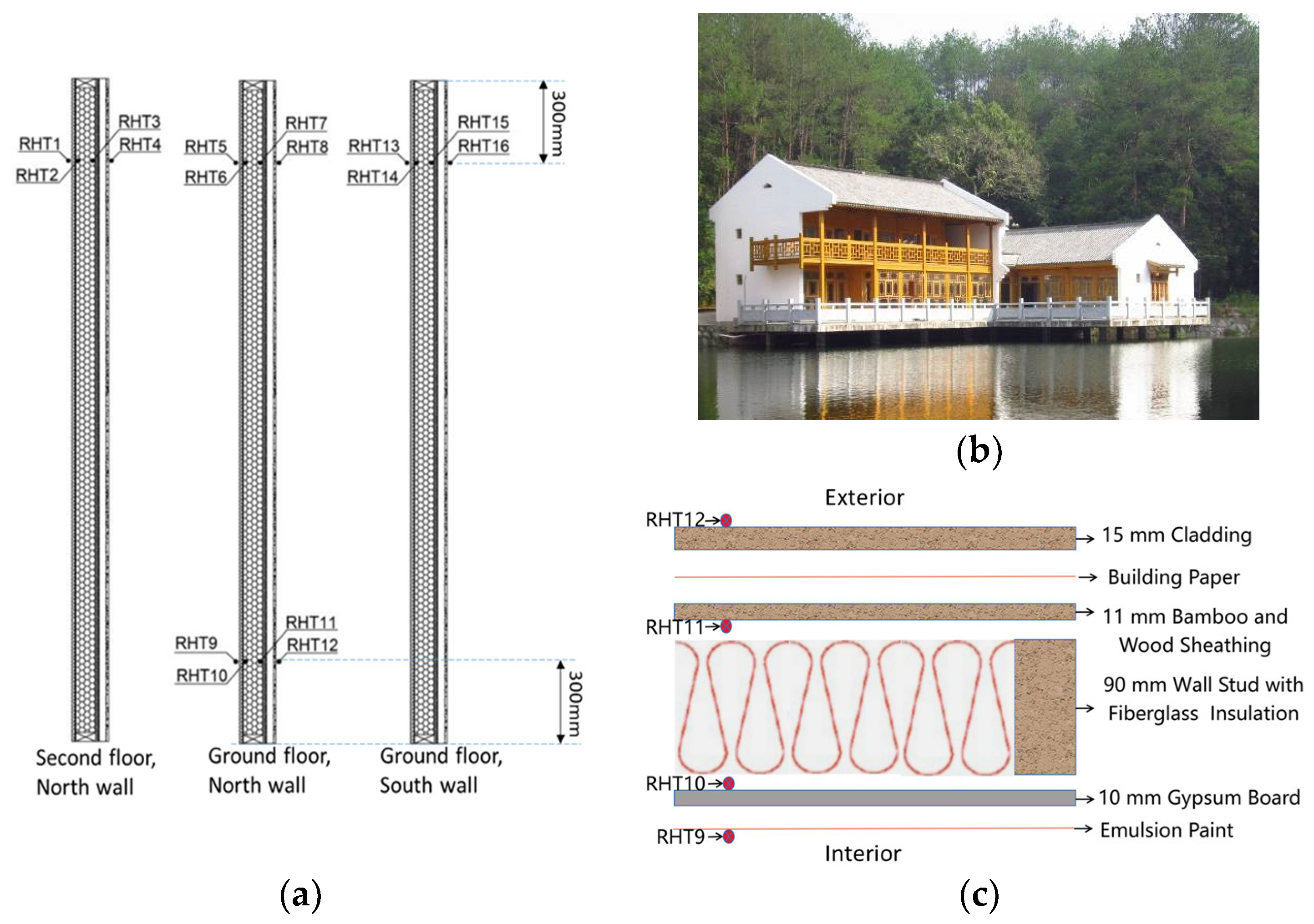
Abstract
:1. Introduction
2. Experimental Setup
2.1. Exterior Wall Configuration and Sensor Installation
2.2. Data Collection
3. Methodology
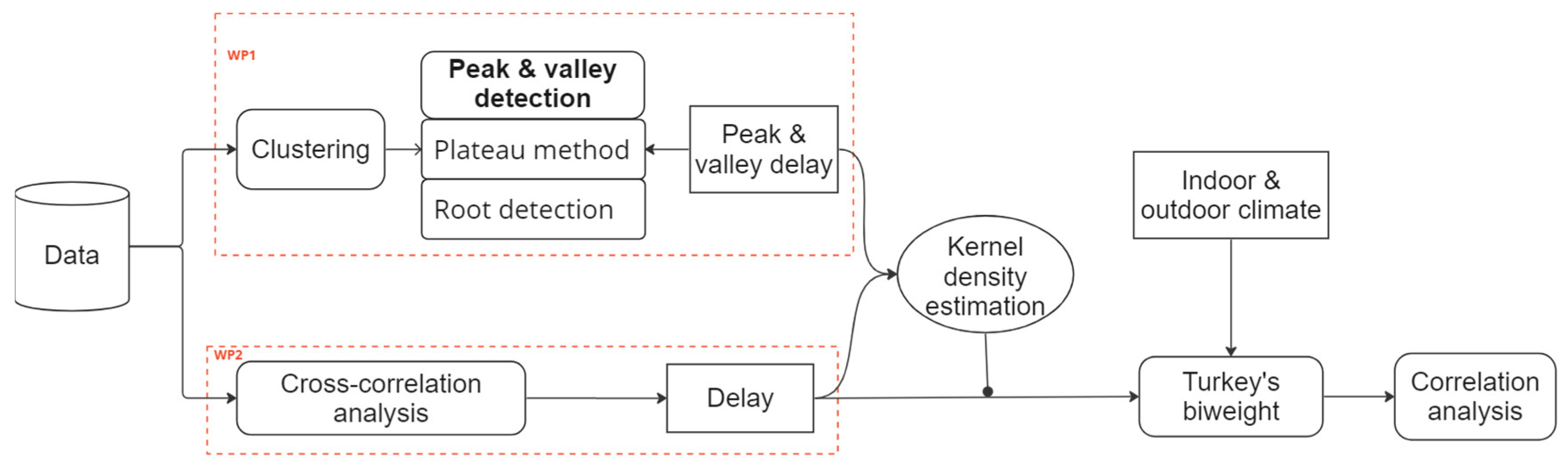
3.1. Methodology Overviews
3.2. WP1
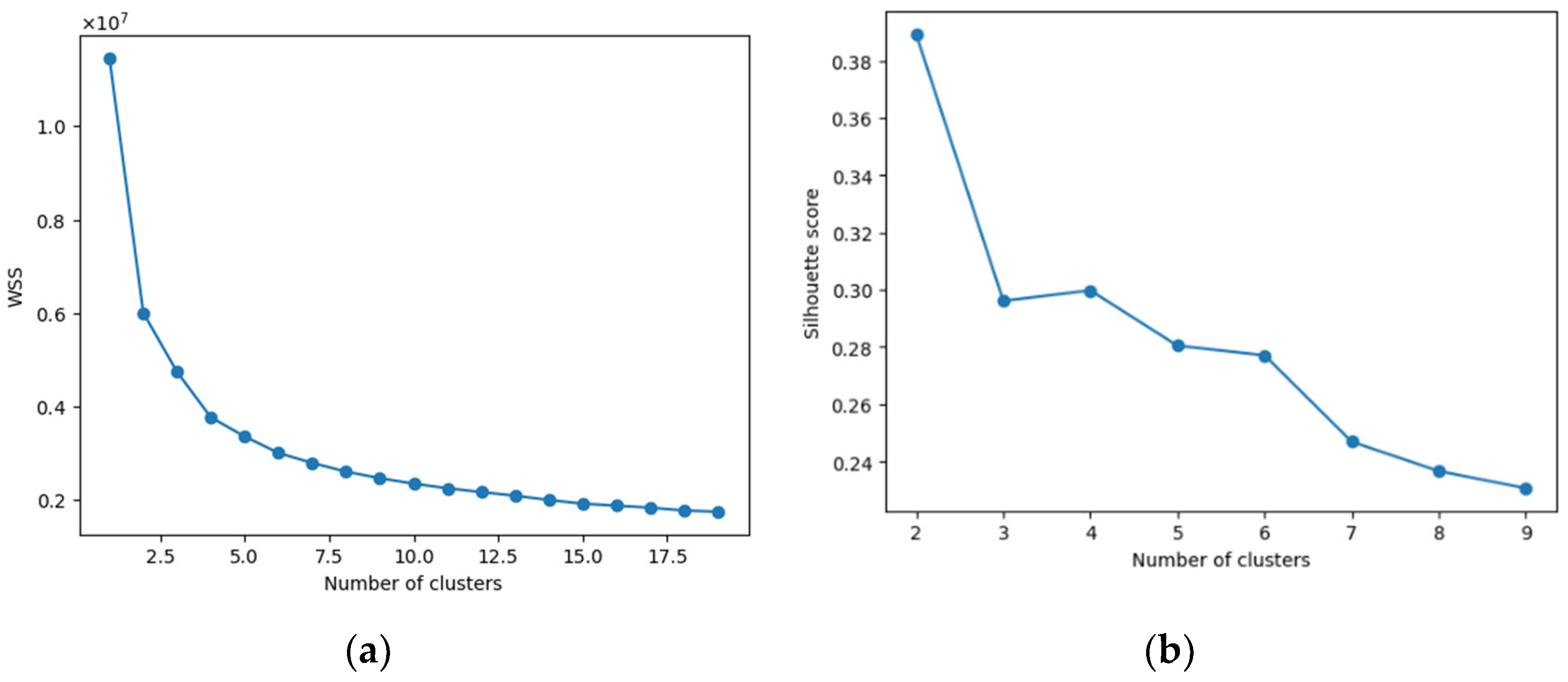
3.2.1. Clustering
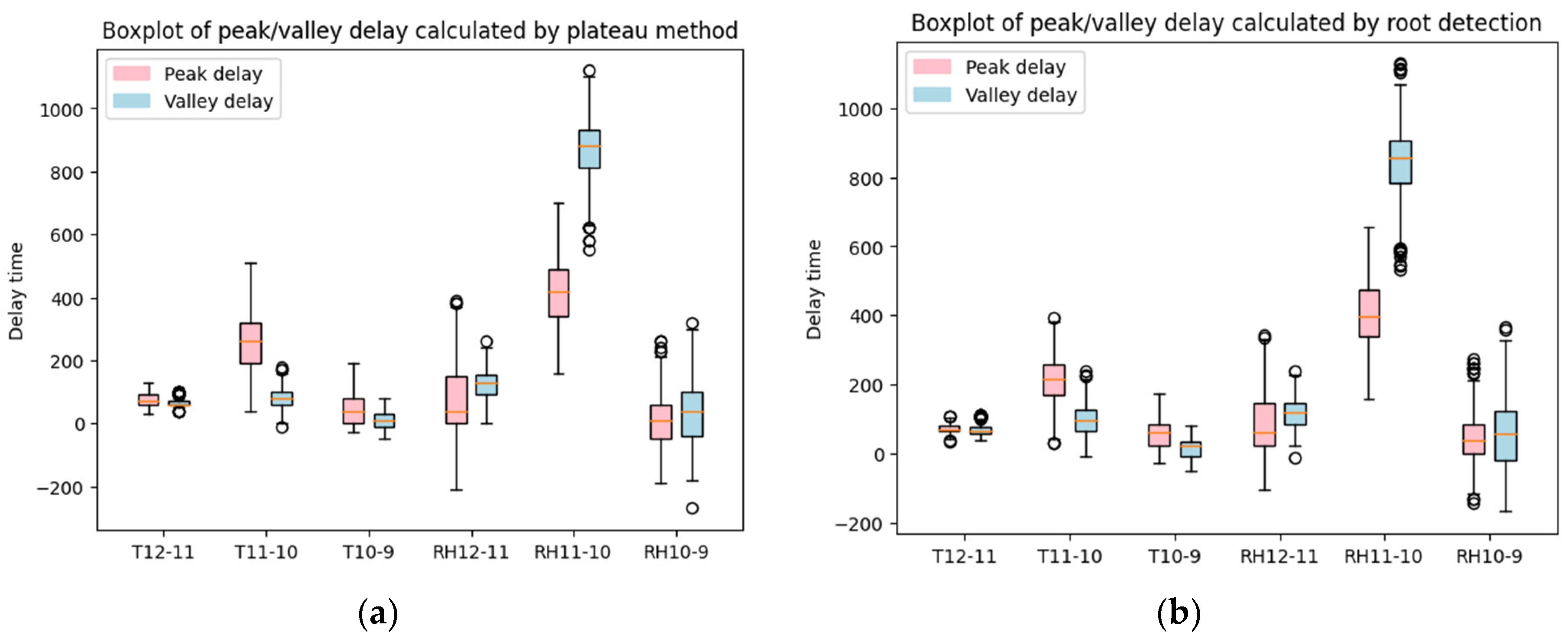
3.2.2. Peak and Valley Detection and Delay Calculation
- Plateau method
- Root Detection
3.3. WP2
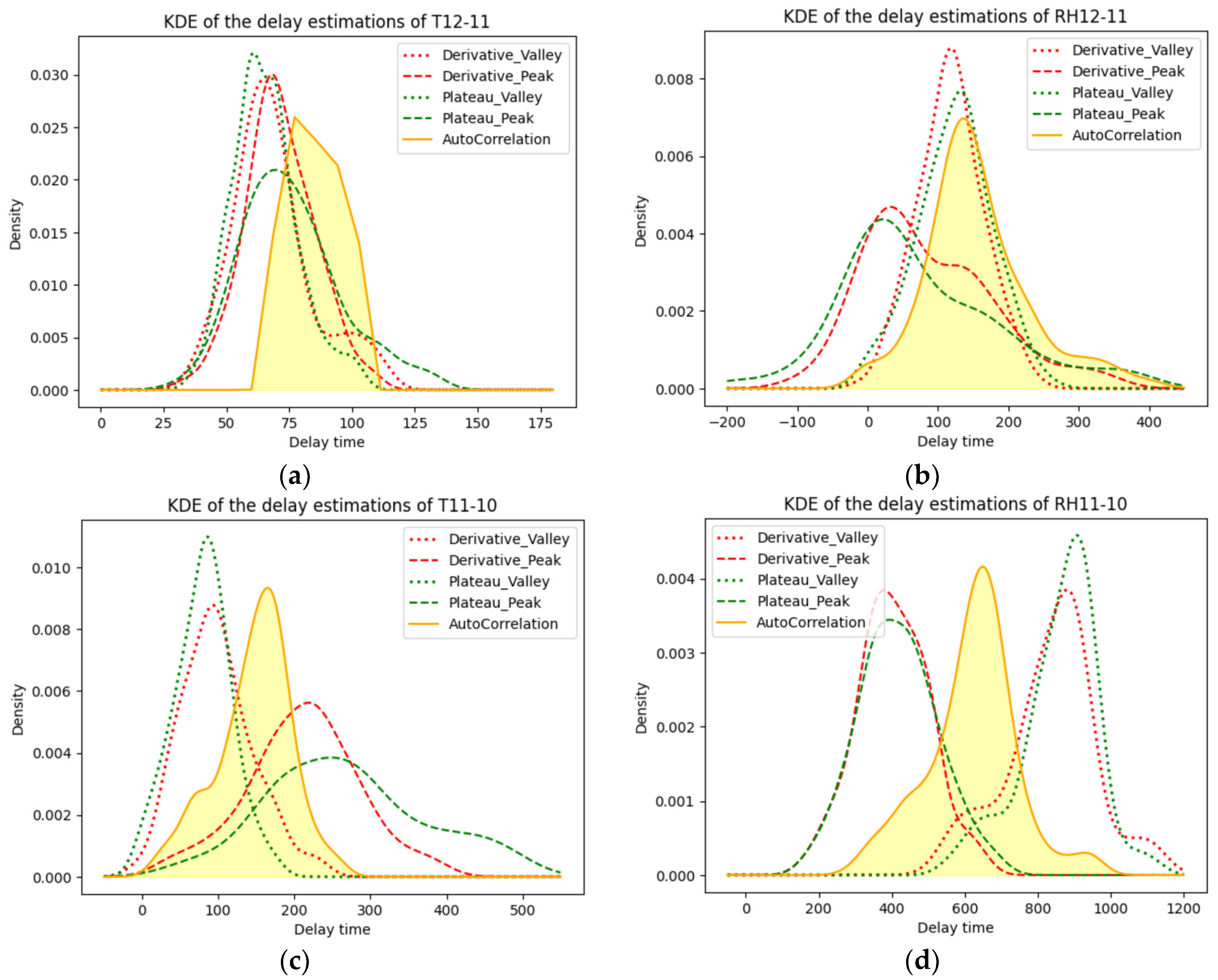
3.4. Kernel Density Estimation
3.5. Tukey’s Biweight
4. Results and Discussion
4.1. WP1
4.1.1. Clustering
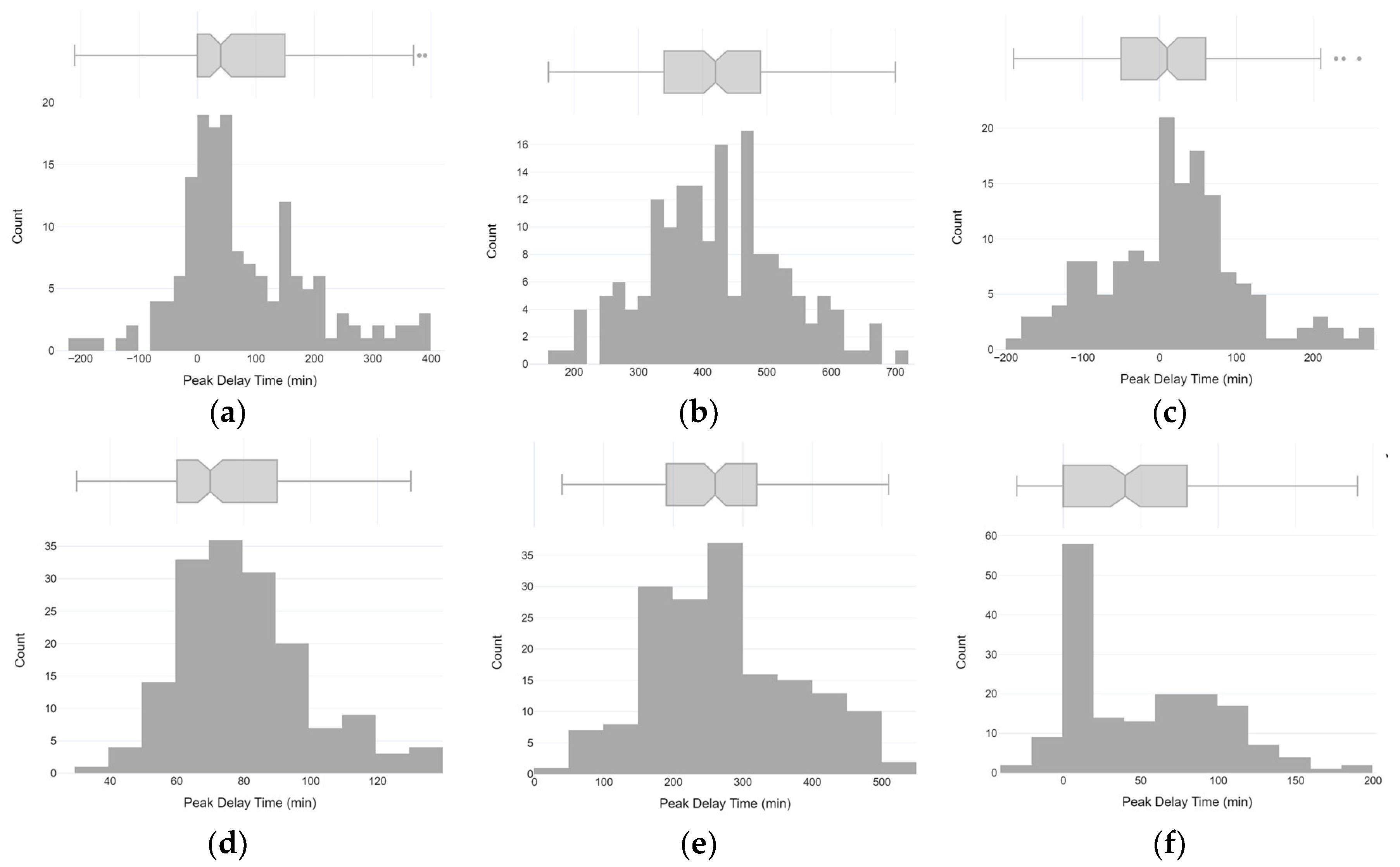
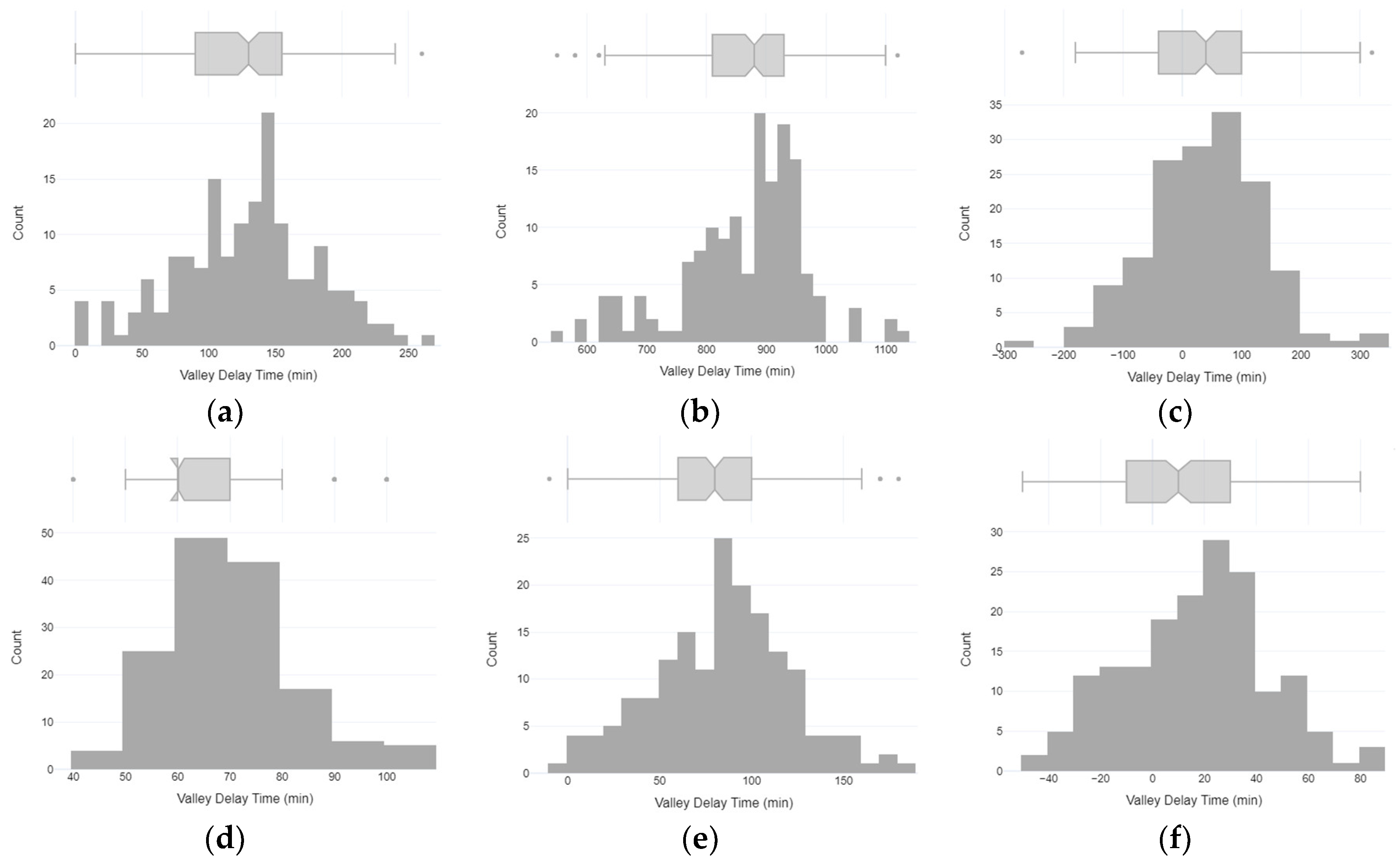
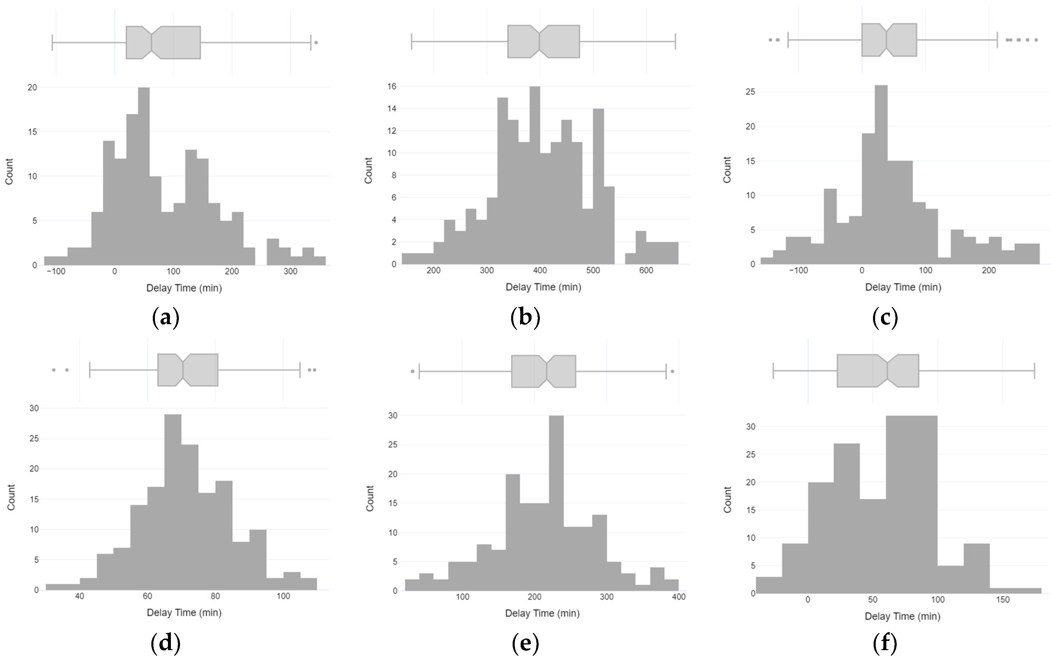
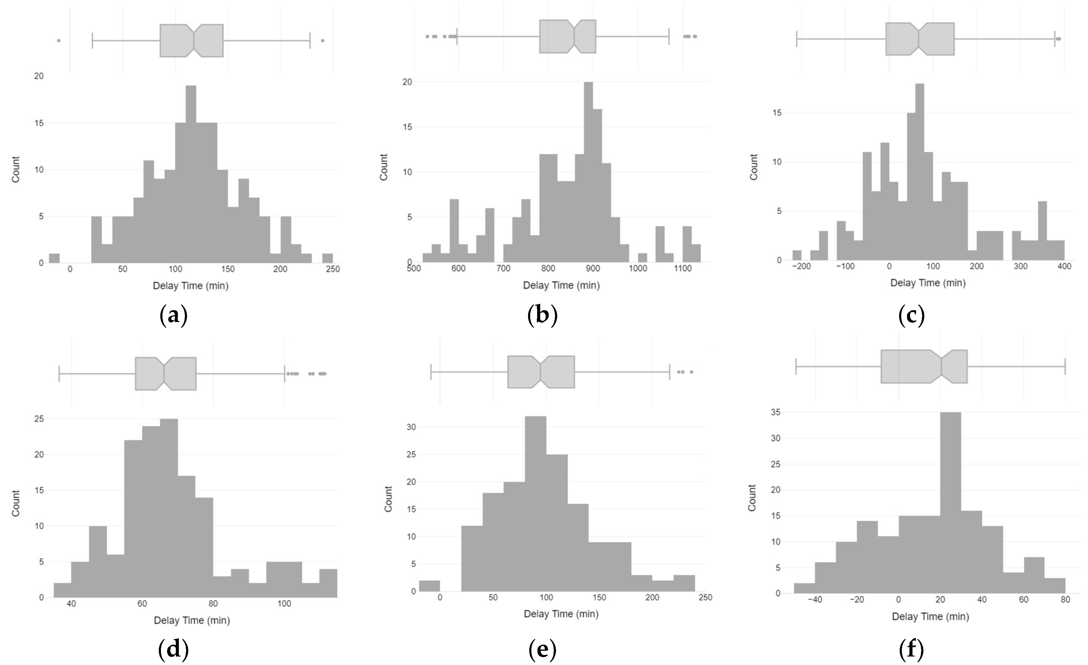
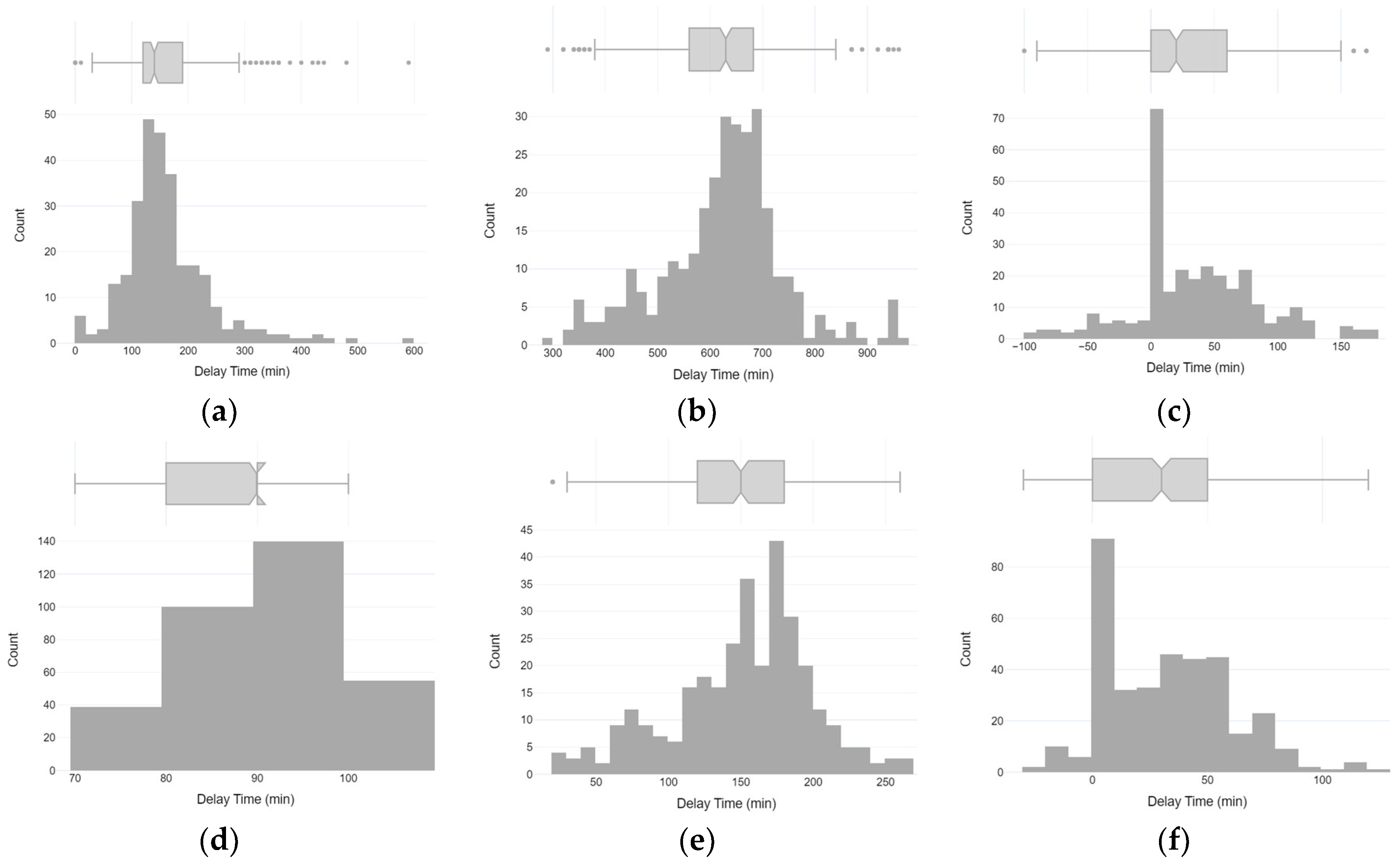
4.1.2. Peak and Valley Delay
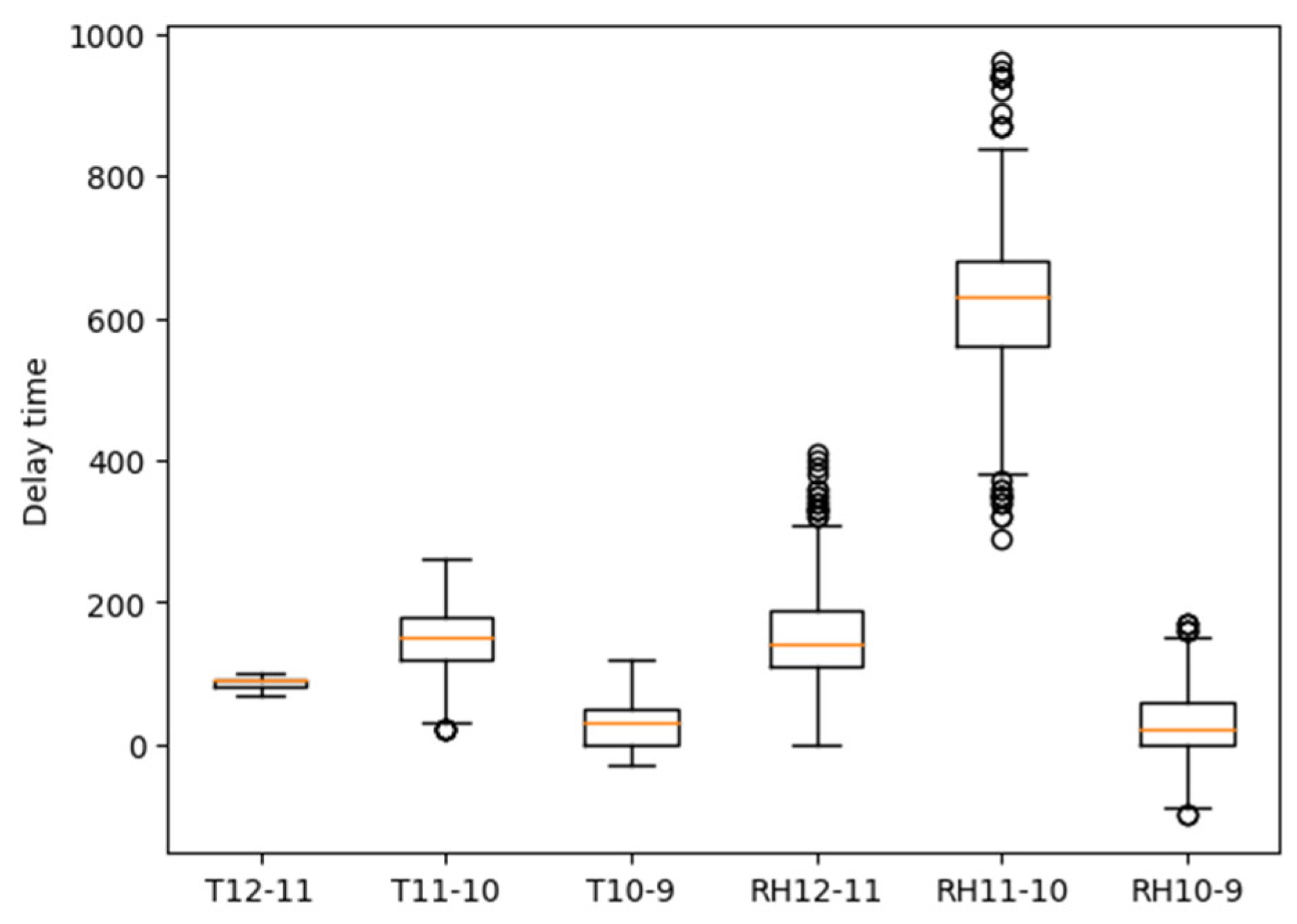
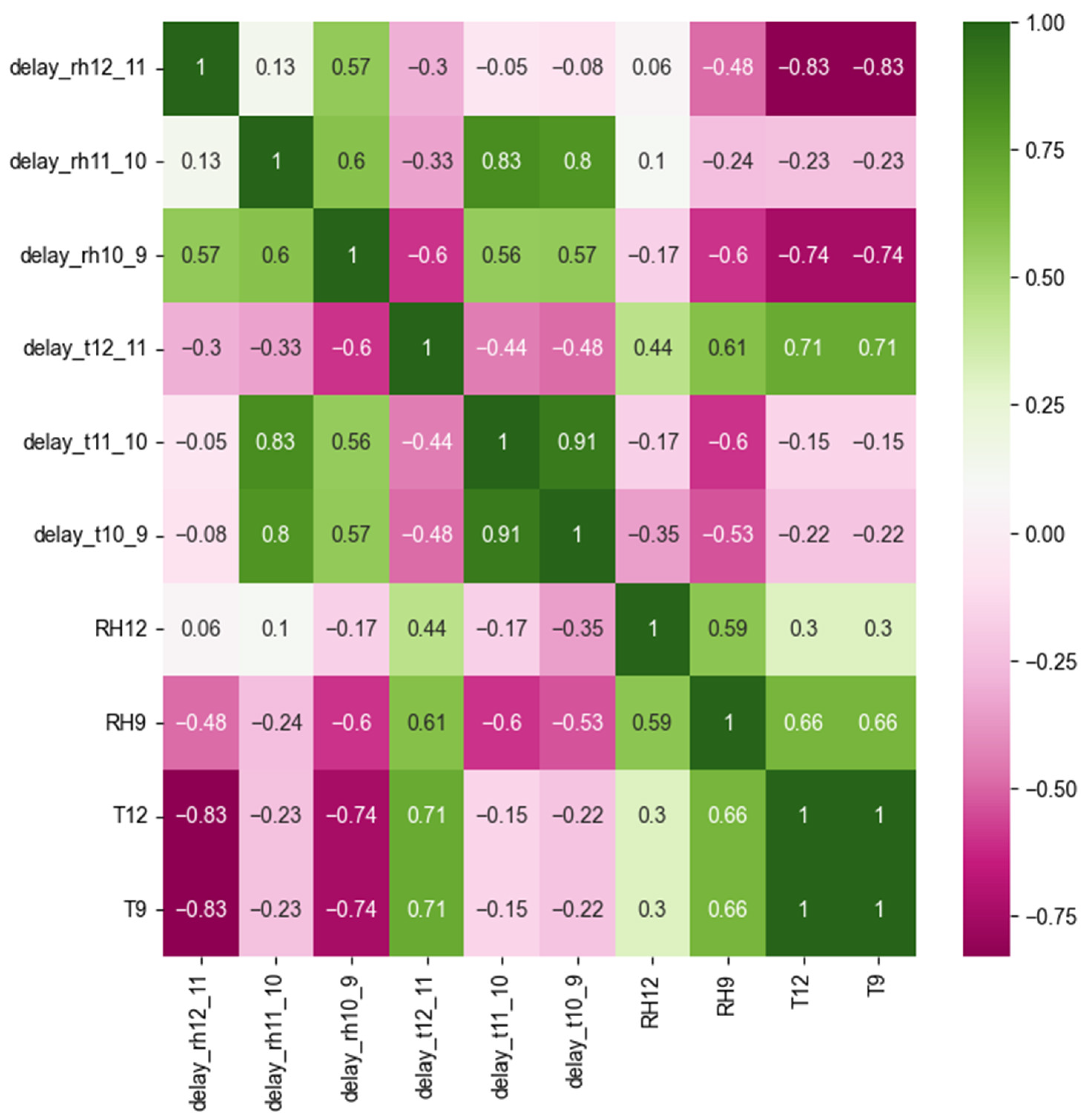
4.2. WP2
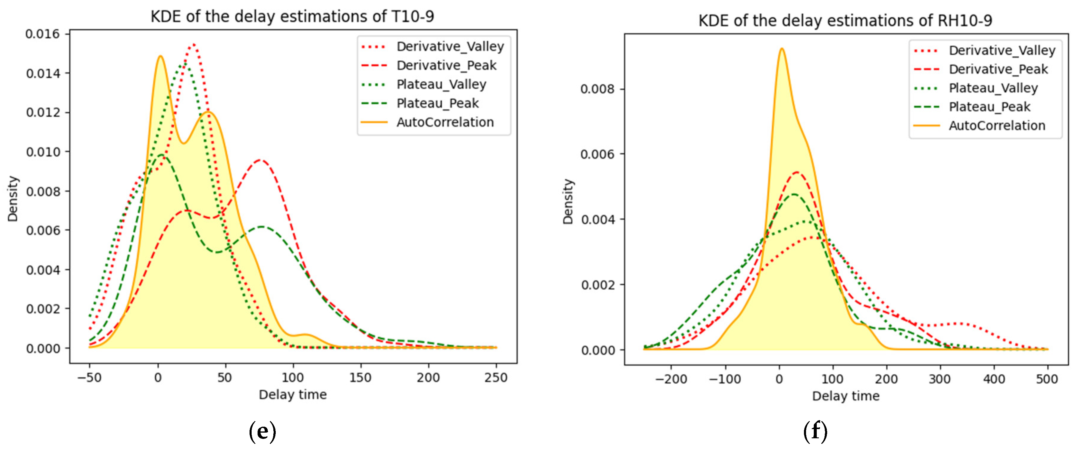
4.3. Kernal Density Estimation
4.4. Transfer Patterns at Monthly Scale
5. Conclusions
Author Contributions
Funding
Data Availability Statement
Conflicts of Interest
Appendix A
Appendix A.1

Appendix A.2

Appendix A.3

Appendix A.4

Appendix B

References
- Nejat, P.; Jomehzadeh, F.; Taheri, M.M.; Gohari, M.; Majid, M.Z.A. A global review of energy consumption, CO2 emissions and policy in the residential sector (with an overview of the top ten CO2 emitting countries). Renew. Sustain. Energy Rev. 2015, 43, 843–862. [Google Scholar] [CrossRef]
- Ibn-Mohammed, T.; Greenough, R.; Taylor, S.; Ozawa-Meida, L.; Acquaye, A. Operational vs. embodied emissions in buildings—A review of current trends. Energy Build. 2013, 66, 232–245. [Google Scholar] [CrossRef]
- Brambilla, A.; Sangiorgio, A. Moisture and Buildings: Durability Issues, Health Implications and Strategies to Mitigate the Risks; Woodhead Publishing: Sawston, UK, 2021. [Google Scholar]
- Pihelo, P.; Kalamees, T. The effect of thermal transmittance of building envelope and material selection of wind barrier on moisture safety of timber frame exterior wall. J. Build. Eng. 2016, 6, 29–38. [Google Scholar] [CrossRef]
- Antonyová, A.; Korjenic, A.; Antony, P.; Korjenic, S.; Pavlušová, E.; Pavluš, M.; Bednar, T. Hygrothermal properties of building envelopes: Reliability of the effectiveness of energy saving. Energy Build. 2013, 57, 187–192. [Google Scholar] [CrossRef]
- Taffese, W.Z.; Sistonen, E. Neural network based hygrothermal prediction for deterioration risk analysis of surface-protected concrete façade element. Constr. Build. Mater. 2016, 113, 34–48. [Google Scholar] [CrossRef]
- He, X.; Zhang, H.; Qiu, L.; Mao, Z.; Shi, C. Hygrothermal performance of temperature-humidity controlling materials with different compositions. Energy Build. 2021, 236, 110792. [Google Scholar] [CrossRef]
- Kukk, V.; Kaljula, L.; Kers, J.; Kalamees, T. Designing highly insulated cross-laminated timber external walls in terms of hygrothermal performance: Field measurements and simulations. Build. Environ. 2022, 212, 108805. [Google Scholar] [CrossRef]
- Hamdaoui, M.-A.; Benzaama, M.-H.; El Mendili, Y.; Chateigner, D. A review on physical and data-driven modeling of buildings hygrothermal behavior: Models, approaches and simulation tools. Energy Build. 2021, 251, 111343. [Google Scholar] [CrossRef]
- Tijskens, A.; Roels, S.; Janssen, H. Neural networks for metamodelling the hygrothermal behaviour of building components. Build. Environ. 2019, 162, 106282. [Google Scholar] [CrossRef]
- Tijskens, A.; Roels, S.; Janssen, H. Hygrothermal assessment of timber frame walls using a convolutional neural network. Build. Environ. 2021, 193, 107652. [Google Scholar] [CrossRef]
- Tzuc, O.M.; Gamboa, O.R.; Rosel, R.A.; Poot, M.C.; Edelman, H.; Torres, M.J.; Bassam, A. Modeling of hygrothermal behavior for green facade’s concrete wall exposed to nordic climate using artificial intelligence and global sensitivity analysis. J. Build. Eng. 2021, 33, 101625. [Google Scholar] [CrossRef]
- Wang, X.; Li, H.; Zhu, Y.; Peng, X.; Wan, Z.; Xu, H.; Nyberg, R.G.; Song, W.W.; Fei, B. Using Machine Learning Method to Discover Hygrothermal Transfer Patterns from the Outside of the Wall to Interior Bamboo and Wood Composite Sheathing. Buildings 2022, 12, 898. [Google Scholar] [CrossRef]
- Song, W.; Zhu, Y.; Wang, X.; Peng, X. An Investigation into Effective Data Analysis Methods for Sensor Datasets of a Sample Building. In Proceedings of the 5th International Conference on Big Data Technologies, Qingdao, China, 23–25 September 2022; pp. 125–130. [Google Scholar]
- Likas, A.; Vlassis, N.; Verbeek, J.J. The global k-means clustering algorithm. Pattern Recognit. 2003, 36, 451–461. [Google Scholar] [CrossRef]
- Campbell, J.Y.; Lo, A.W.; MacKinlay, A.C.; Whitelaw, R.F. The econometrics of financial markets. Macroecon. Dyn. 1998, 2, 559–562. [Google Scholar] [CrossRef]
- Wand, M.P.; Jones, M.C. Kernel Smoothing; CRC Press: Boca Raton, FL, USA, 1994. [Google Scholar]
- Scott, D.W. Multivariate Density Estimation: Theory, Practice, and Visualization; Wiley: New York, NY, USA, 1992. [Google Scholar]
- Flannery, B.P.; Press, W.H.; Teukolsky, S.A.; Vetterling, W. Numerical recipes in C; Press Syndicate of the University of Cambridge: New York, NY, USA, 1992; Volume 24, p. 36. [Google Scholar]
- Thybring, E.E.; Fredriksson, M.; Zelinka, S.L.; Glass, S.V. Water in wood: A review of current understanding and knowledge gaps. Forests 2022, 13, 2051. [Google Scholar] [CrossRef]
- Dinçer, İ.; Zamfirescu, C. Drying Phenomena: Theory and Applications; John Wiley & Sons: Hoboken, NJ, USA, 2016. [Google Scholar]
- Peuhkuri, R. Moisture Dynamics in Building Envelopes. Ph.D. Thesis, Technical University of Denmark, Lyngby, Denmark, 2003. [Google Scholar]


Disclaimer/Publisher’s Note: The statements, opinions and data contained in all publications are solely those of the individual author(s) and contributor(s) and not of MDPI and/or the editor(s). MDPI and/or the editor(s) disclaim responsibility for any injury to people or property resulting from any ideas, methods, instructions or products referred to in the content. |
© 2023 by the authors. Licensee MDPI, Basel, Switzerland. This article is an open access article distributed under the terms and conditions of the Creative Commons Attribution (CC BY) license (https://creativecommons.org/licenses/by/4.0/).
Share and Cite
Zhu, Y.; Song, W.; Wang, X.; Rybarczyk, Y.; Nyberg, R.G.; Fei, B. A Novel Approach to Discovering Hygrothermal Transfer Patterns in Wooden Building Exterior Walls. Buildings 2023, 13, 2151. https://doi.org/10.3390/buildings13092151
Zhu Y, Song W, Wang X, Rybarczyk Y, Nyberg RG, Fei B. A Novel Approach to Discovering Hygrothermal Transfer Patterns in Wooden Building Exterior Walls. Buildings. 2023; 13(9):2151. https://doi.org/10.3390/buildings13092151
Chicago/Turabian StyleZhu, Yurong, Wei Song, Xiaohuan Wang, Yves Rybarczyk, Roger G. Nyberg, and Benhua Fei. 2023. "A Novel Approach to Discovering Hygrothermal Transfer Patterns in Wooden Building Exterior Walls" Buildings 13, no. 9: 2151. https://doi.org/10.3390/buildings13092151