Identification of Tension Force in Cable Structures Using Vibration-Based and Impedance-Based Methods in Parallel

Abstract

For cable structures, the tension force is one of the main factors showing the structure’s health. If the tension force falls below a safe level during construction or operation, it can lead to partial or complete the structural failure, posing a risk to the people’s safety. In this study, a parallel structural health monitoring approach of the vibration-based and impedance-based methods is proposed to identify the tension force in cable structures. Firstly, a cable structure including the anchorage is simulated using a finite element model to obtain the vibration and impedance responses. The numerical results are verified with the experimental ones of the previous studies. Then, the parallel approach combining the above two methods is presented to determine the tension force. For the vibration-based method, the tension force is estimated by the natural frequencies. For the impedance-based method, the tension force is estimated by the mean absolute percentage deviation (MAPD) index and the artificial neural network (ANN). Finally, the tension force estimation results are compared and assessed. By using the parallel approach, the reliability and accuracy of the tension force identification results are guaranteed.

1. Introduction

Nowadays, cables are commonly used for civil infrastructures such as cable-stayed bridges, guyed mast towers, and prestressed concrete structures. In these structures, the tension force is a critical factor in assessing the health of the structures, and the cable anchorage system also plays an essential role in transmitting the tension force to the main structure. However, under the impacts of natural and anthropogenic conditions, the tension force can be lost, including instantaneous losses at the stressed cable stage or time-dependent tension losses, such as anchorage slip, tendon friction and relaxation in girder-bridges. When the tension force loss or the bearing capacity reduction due to the anchor connection’s damage exceeds the safety threshold, it can lead to partial or complete failure of the main structure, which may jeopardize the people’s safety. Therefore, the tension force in cable structures is an important diagnostic target through structural health monitoring (SHM) techniques to ensure the operability of the whole structure. Among SHM techniques, vibration-based and impedance-based methods have been developed for monitoring and evaluating the tension force in cable structures. Then, the structural health is provided timely and measured correctly to ensure the structure works normally.

The tension force in cable structures was first studied in 1974 through the vibration-based method to solve the characteristic free vibration equation of a cable [1]. By different analytical methods and approximations, several methods for determining the cable tension force using natural frequency were presented. In addition, the studies considered the effects of errors of deflection, bending, and flexural stiffness on the vibration equation [2,3,4,5,6]. The asymptotic forms of the vibration equation are improved to effectively monitor the vibration of the cable structures on site, which was verified by experimental data of a cable-stayed bridge in Vietnam [7,8]. Recently, Liang et al. introduced the impedance-based method to detect structural damage by the electro-mechanical interaction between PZT (lead zirconate titanate) sensor and the host structure [9]. After that, other studies related to the high-frequency range, the shape of the sensor, the appropriate damage assessment index were conducted to evaluate the loss of tension force on the cables [10,11,12,13]. In addition, the cable anchorage models were simulated and compared with experiments to verify the model’s reliability and effectiveness [14,15,16]. Moreover, damage detection models were applied and combined with the impedance-based method to accurately determine the damages in various structures, such as cable-anchorage [17,18], tendon-anchorage [19,20,21], bolted connections [22], long cables [23], concrete structures [24,25,26,27,28]. Presently, the machine learning techniques were employed for the feature extraction with the impedance-based method to efficiently detect damages or cracks in structures [29,30]. Among those previous studies, the following questions remain unsolved for the health condition assessment of cable structures: (1) Are the calculation results obtained from the numerical simulation consistent with the experimental values in the vibration-based method? (2) How to identify and evaluate the tension force of cable structures by using the impedance-based method? (3) How reliable is the parallel approach of the vibration-based and impedance-based methods to identify the tension force?

In order to address the aforementioned questions, this paper establishes three problems to identify the tension force of the cable structures using the vibration-based and impedance-based techniques in parallel. Firstly, a cable structure is simulated by the finite element method. Then, the cable tension is calculated based on the natural frequencies derived from the simulation. The accuracy of the numerical results is verified by comparing them with the experimental data from the previous study. Secondly, the cable’s anchorage system is simulated using the finite element method. The potential loss of cable tension is evaluated using the mean absolute percentage deviation (MAPD) index based on the impedance responses obtained from the simulation. The numerical impedance-based results are also verified with the previous study’s experiments. Then, the cable tension is predicted by using the artificial neural network (ANN) with impedance responses as the input data. Finally, the reliability of the parallel approach is evaluated from the tension force results identified by vibration-based and impedance-based methods.

The research and development of different methods to identify the structural damages are essential. The vibration-based SHM methods are suitable for detecting the global structural damages and are investigated in the low-frequency range. Meanwhile, the impedance-based SHM methods are suitable for detecting the local structural damages and are investigated in the high-frequency range. In the previous studies, the cable tension was identified separately using either the vibration-based method or the impedance-based method. The utilization of only one method may result in misdiagnosis or confusion. The novelty of this study lies in the simultaneous identification of cable tension using both vibration-based and impedance-based methods. The results of the two methods complement each other. The cross-checking result enhances the reliability of the structural health monitoring process.

2. Cable Force Identification Using Vibration-Based and Impedance-Based Methods

2.1. The Vibration-Based Method

The vibration-based method offers an indirect way to determine the cable tension instead of relying on direct methods or visual inspection. This technique involves monitoring the vibration and deformation of the cable structures by using accelerometers or fiber optic sensors placed on the cable. By exciting the cable structure with a vibrated force, the natural frequencies of the cable are obtained. The cable tension is then determined using the natural frequencies. The cable is stretched in an inclined direction by an angle $\theta \left(0\le \theta \le \pi /2\right)$ under the tension force $T$ (Figure 1). A coordinate system is established with the origin at point A, the x-axis along the AB, and the y-axis perpendicular to the x-axis. The cable has a mass per unit length $m$, a length in the AB direction $L$, an elastic modulus of the rope material $E$, a constant cross-sectional moment of inertia $I$, and a slack at vertical mid-span $s$. The following assumptions are mentioned, including that the ratio of the slack to the span of the cable is minimal $\delta =s/L_o\ll 1$, the cable only vibrates in the (Axy) plane, and the displacement in the x direction is negligible. Additionally, the geometrical characteristic of the cable is assumed to be a quadratic parabola.

Shimada (1994) [3] proposed the displacement equation of the cable in the y direction:

$$EI\frac{{\partial }^{4}v\left(x,t\right)}{\partial x^4}-T\frac{{\partial }^{2}v\left(x,t\right)}{\partial x^2}-h\left(t\right)\frac{{\partial }^{2}y}{\partial x^2}+m\frac{{\partial }^{2}v\left(x,t\right)}{\partial t^2}=0$$

(1)

where $EI$ is the flexural stiffness of the cable; $v\left(x,t\right)$ is the displacement in the y direction of the cable at the position of x coordinate at time t when the cable vibrates; $T$ is the cable tension in the AB direction; $h\left(t\right)$ is the increased tension generated in the cable due to the vibration. After applying the analytical methods, the practical formulas for calculating the cable tension were derived. The parameters $\xi$ and Γ are calculated from cable characteristics and design state. The different vibration shapes are concerned depending on the value of Γ. The practical formulas for determining the cable tension by Zui et al. (1996) [4] are suggested as follows:

For the first mode:

$$T=4m{\left(f_{1}L\right)}^2\left[1-2.2\frac{C}{f_1}-0.55{\left(\frac{C}{f_1}\right)}^2\right];\left(\xi >17\right)$$

(2)

$$T=4m{\left(f_{1}L\right)}^2\left[0.865-11.6{\left(\frac{C}{f_1}\right)}^2\right];\left(6<\xi \le 17\right)$$

(3)

$$T=4m{\left(f_{1}L\right)}^2\left[0.828-10.5{\left(\frac{C}{f_1}\right)}^2\right];\left(0\le \xi \le 6\right)$$

(4)

For the second mode:

$$T=m{\left(f_{2}L\right)}^2\left[1-4.4\frac{C}{f_2}-1.1{\left(\frac{C}{f_2}\right)}^2\right];\left(\xi >60\right)$$

(5)

$$T=m{\left(f_{2}L\right)}^2\left[1.03-6.33\frac{C}{f_2}-1.58{\left(\frac{C}{f_2}\right)}^2\right];\left(17<\xi \le 60\right)$$

(6)

$$T=m{\left(f_{2}L\right)}^2\left[0.882-85{\left(\frac{C}{f_2}\right)}^2\right];\left(0\le \xi \le 17\right)$$

(7)

For the higher-order mode:

$$T=\frac{4m}{n^2}{\left(f_{n}L\right)}^2\left[1-2.2n\frac{C}{f_n}\right];\left(\xi \ge 200\right)$$

(8)

where $f_1, f_2, f_n$ are the natural frequency of the 1st mode, the 2nd mode, and the nth mode, respectively; $\xi =L\sqrt{\left(T/EI\right)}$, $C=\sqrt{\left(EI/m{L}^4\right)},$ and $\mathsf{\Gamma }=\sqrt{\frac{mgL}{128EA{\delta }^{3}co{s}^5\theta }}\times \frac{0.31\xi +0.5}{0.31\xi -0.5}$.

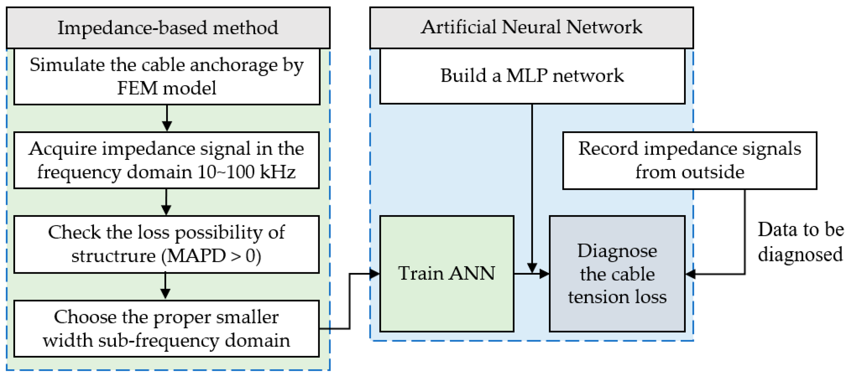
2.2. The Impedance-Based Method

2.2.1. Electro-Mechanical Impedance Responses

The impedance technique uses piezoelectric materials to identify and evaluate minor defects in structures that are not easily visible. The impedance-based methods detect the changes in electro-mechanical impedance responses, which occurs in the high-frequency domain. These impedance responses are characterized by the interplay between the capacitance of the piezoelectric materials and the mechanical interaction of the structure, such as mass, stiffness, damping, and boundary conditions. Piezoelectric materials generate an electric field when subjected to mechanical strain or friction (direct piezoelectric effect), conversely, they undergo mechanical strain when an electric field is applied (inverse piezoelectric effect). They contain positive and negative ions in pairs forming ionic bonds, which come in various forms such as crystalline (e.g., LiTaO₃, GaPO₄, and NH₄H₂PO₄), ceramic (e.g., PZT-5A, PZT 5-H, and BiFeO₃), and polymeric (e.g., PVDF). Among these, PZT ceramics have been frequently used in SHM due to their high sensitivity and suitability for high-frequency applications.

For an anchorage system, the PZT sensor is bonded to an interface affixed to the anchorage using a high-strength adhesive to ensure the optimal mechanical interaction and to capture the dynamic responses directly (Figure 2a). The use of the aluminum interface improves the sensitivity of the impedance responses when the cable tension changes [19,20,21]. The PZT sensor works under the direct piezoelectric effect by supplying a fixed electric field. When the structural damages appear, the dynamic responses of the host structure change at high frequency, leading to a corresponding change in the electrical response of the PZT sensor. In Figure 2b, the PZT sensor is described as a short-circuit source with harmonic voltage $V\left(\omega \right)$ and amperage $I\left(\omega \right)$. The electro-mechanical impedance $Z\left(\omega \right)$, is the combined function of the impedance of the anchorage and interface $Z_{a,i}\left(\omega \right)$ and the PZT sensor $Z_{pzt}\left(\omega \right)$ which is expressed as follows:

$$Z\left(\omega \right)=\frac{V\left(\omega \right)}{I\left(\omega \right)}={\left[i\omega \frac{w_{pzt}{t}_{pzt}}{l_{pzt}}\left({\overline{\epsilon }}_{33}^T-\frac{Z_{a,i}\left(\omega \right)}{Z_{a,i}\left(\omega \right)+Z_{pzt}\left(\omega \right)}{d}_{32}^2{\overline{Y}}_{22}^E\right)\right]}^{-1}$$

(9)

where $w_{pzt}, t_{pzt}, l_{pzt}$ are the width, the thickness, the length of the PZT sensor, respectively; ${\overline{Y}}_{22}^E=Y_{22}^E\left(1+i\eta \right)$ is the modulus of the PZT sensor at zero electric field; $\eta$ is the drag coefficient of the PZT sensor; ${\overline{\epsilon }}_{33}^T={\epsilon }_{33}^T\left(1-i\delta \right)$ is the dielectric coefficient of the PZT sensor when the stress is zero; $\delta$ is the dielectric loss coefficient; $d_{32}$ is the piezoelectric coefficient of the PZT sensor when the stress is zero.

The size of the PZT sensor and its material characteristics, such as the elastic strain, the dielectric coupling constant, the dielectric constant, the drag coefficient, and the dielectric loss coefficient, affect the electro-mechanical impedance. In addition, the material characteristics of the interface, bearing plate, and anchor head also play a significant role in the impedance responses. When the PZT impedance $Z_{pzt}\left(\omega \right)$ and the structural impedance $Z_{a,i}\left(\omega \right)$ coincide, the electro-mechanical system resonates, causing changes in the mechanical impedance of the anchorage due to cable tension change. The electro-mechanical impedance is a complex function that includes the real part and the imaginary part. Bhalla and Soh (2003) [5] proved that the real part of the impedance was more sensitive to structural damage. As a result, the real part of the impedance has usually been used to represent the impedance responses for structural damage detection purposes.

2.2.2. The Impedance-Based Damage Index

The change in impedance responses evaluating the cable structure’s tension force loss can be quantified through different statistical techniques and evaluation indicators. This study employs the mean absolute percentage deviation (MAPD) index to evaluate the loss of cable tension in regression analysis and model evaluation. The MAPD index is calculated by comparing the impedance responses before and after the loss of cable tension occurs. The MAPD index larger than 0 indicates the presence of cable tension loss. The formula for calculating the MAPD index is as follows:

$$MAPD(\%)=\frac{1}{n}{\displaystyle \sum }_{i=1}^n\left|\frac{Z^{*}\left({\omega }_i\right)-Z\left({\omega }_i\right)}{Z\left({\omega }_i\right)}\right|\times 100$$

(10)

where $Z\left({\omega }_i\right)$ and $Z^{*}\left({\omega }_i\right)$ are the impedance responses received from the PZT sensor attached to the anchorage system before and after the cable tension loss, respectively.

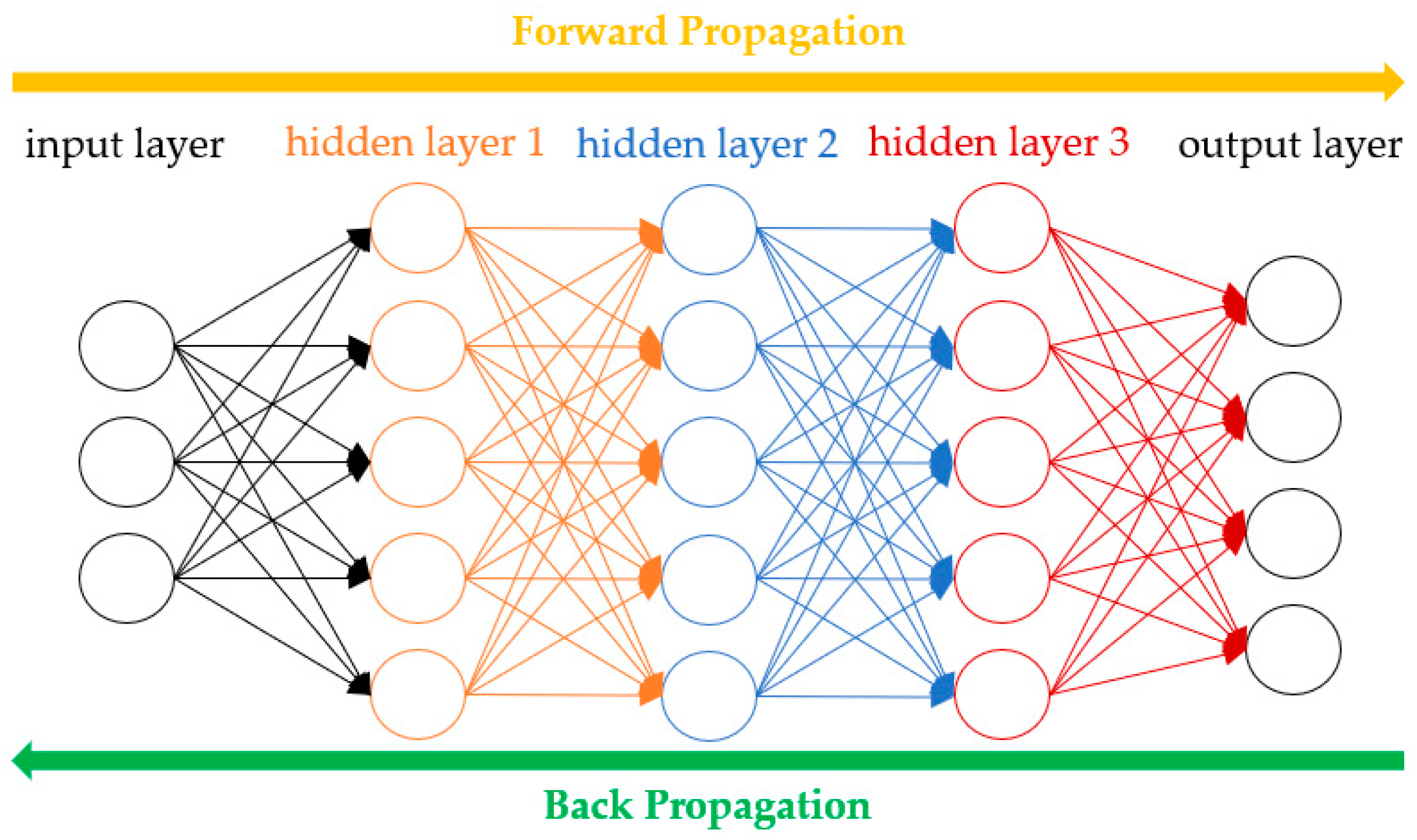
2.2.3. The Artificial Neural Network

The artificial neural network (ANN) is a deep learning technique of artificial intelligence, which is a series of algorithms designed to identify basic relationships in a set of data. By imitating the way a neuron in the human brain works, a typical artificial network (Figure 3) or a perceptron is composed of five main components:

(1) Input data: Each input value corresponds to an attribute of the data.

(2) Linking weight: The important component represents the level of the input data in the information processing. The learning process of ANN is the process of adjusting the weights of the input data to get the desired output through a back-propagation algorithm called gradient descent.

(3) Sum function: The sum of weights of all the values fed into each neuron. The sum function of a neuron for n input values is calculated according to the following formula:

$$z_j={\sum }_{i=1}^n{w}_{ij}{x}_i+w_j$$

(11)

(4) Transfer function: The sum function of a neuron shows the internal activation capacity of that neuron. In which, the sigmoid and hyperbolic tangent functions are two functions that give better reliable diagnostic results, which are used in this study to predict the cable tension.

(5) Output data: The output value of a neuron, which is the result that has been fed into the transfer function.

The most commonly used the ANN model is the multi-layers perception (MLP) network. The MLP network is a forward transmission network consisting of N layers of perceptrons (excluding the input layer), in which there are (N – 1) hidden layers and one output layer (the Nth layer). The neuron’s output in the previous layer is the input of the neuron in the next layer (Figure 4).

About the operating principle of ANN, at the input layer, the neurons receive input data for processing with their respective weights and then give the output from the transfer function. This output is then transmitted to the neurons at the first hidden layer, which continues the processing and sends the results to the second hidden layer, etc., until the output layer exports prediction results. In this study, a MLP ANN is built and trained to conduct the cable tension identification through the impedance responses. Following the flowchart in Figure 5, the possibility of cable tension loss at the anchorage is first examined by checking if the MAPD index is larger than 0, the impedance responses in the sub-frequency domain are used as the training dataset for the MLP ANN.

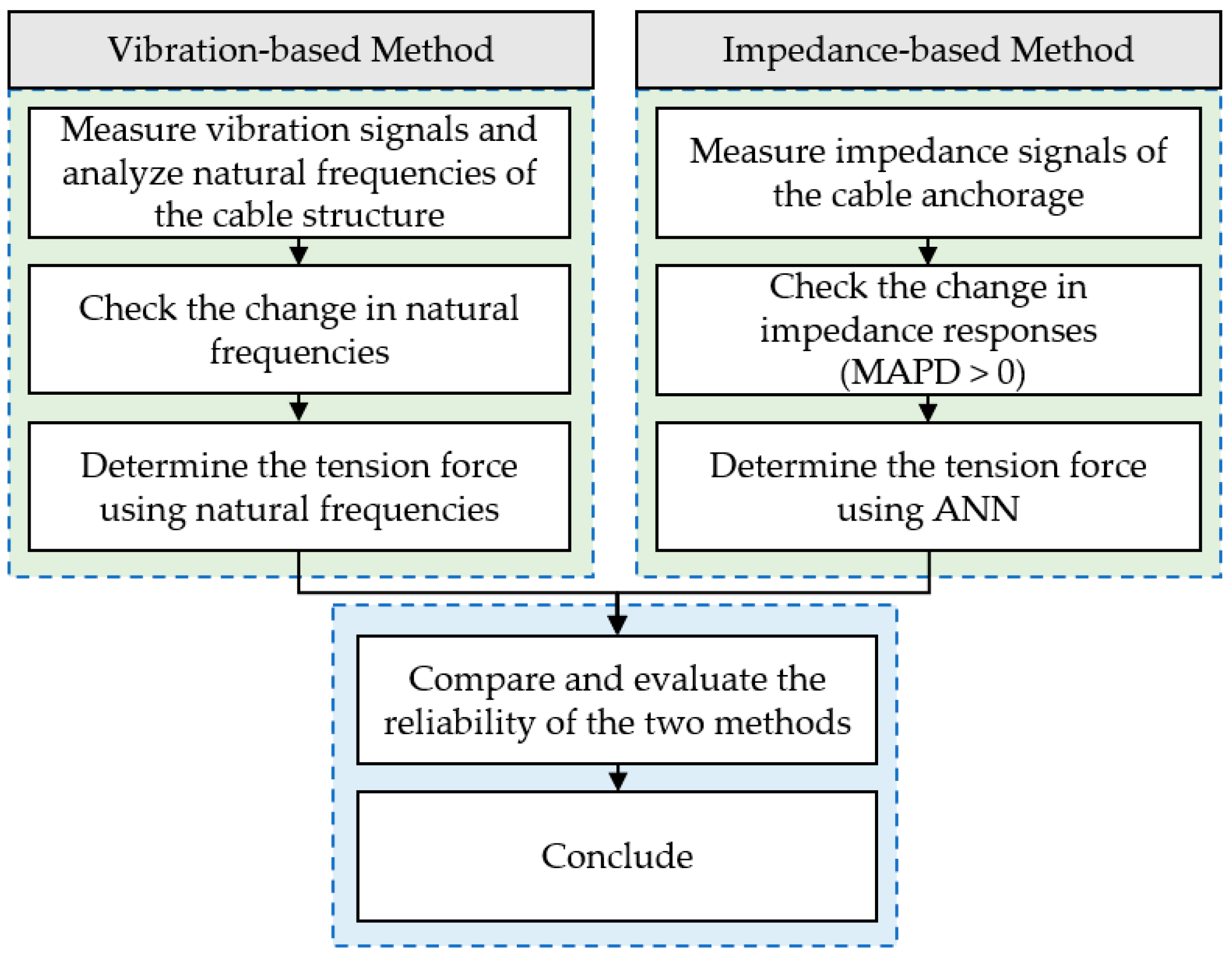
2.3. Vibration-Based and Impedance-Based Parallel Approach

Both the vibration and impedance methods have their advantages and disadvantages. One of the significant advantages of both methods is the ease of access to the host structures and signal response acquisition during the measurement process. In addition, the small and lightweight sensors placed on the cable and interface do not affect the overall performance of the host structure. Therefore, a parallel approach combining the vibration-based and impedance-based methods is proposed to identify the tension force of cable structures based on changes in natural frequencies and impedance responses. In the proposed approach (Figure 6), for the vibration-based method, the cable’s vibration signals (i.e., acceleration) are measured; then, the cable’s natural frequencies are analyzed. The change in natural frequencies is checked, and the cable’s tension force is determined by using the natural frequencies (Equations (2)–(8)). In parallel, for the impedance-based method, the impedance signals are measured from the PZT sensor placed on the interface’s cable anchorage. Then, the possibility of cable tension loss is alarmed by the MAPD index; and the extent of this loss is determined by using MLP ANN. Finally, the cable tension identification results from both methods are compared, and the reliability of the results is evaluated. If the identification results show a low difference, the tension force and the cable tension loss are confirmed.

3. Verifications

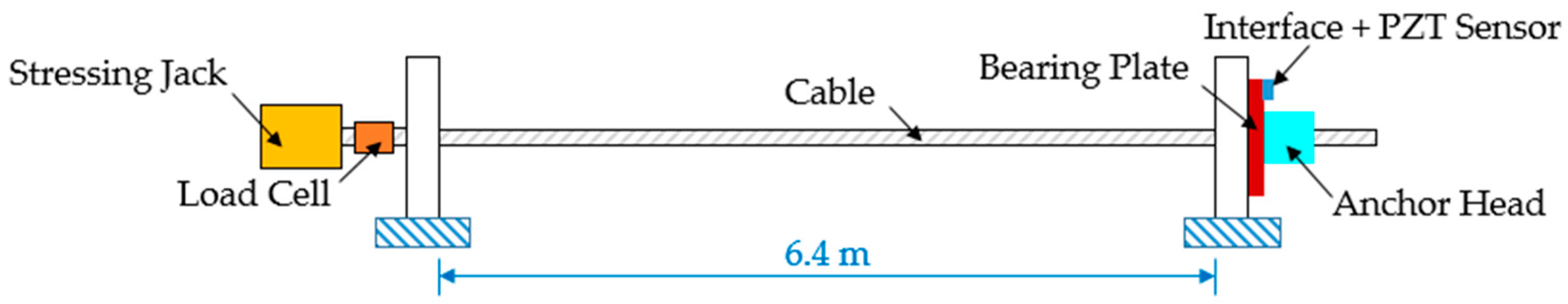
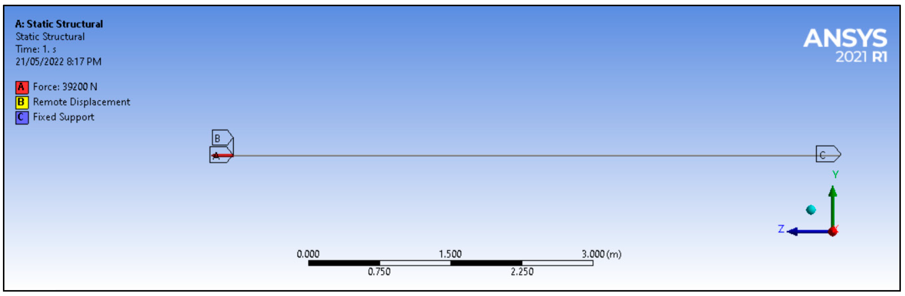
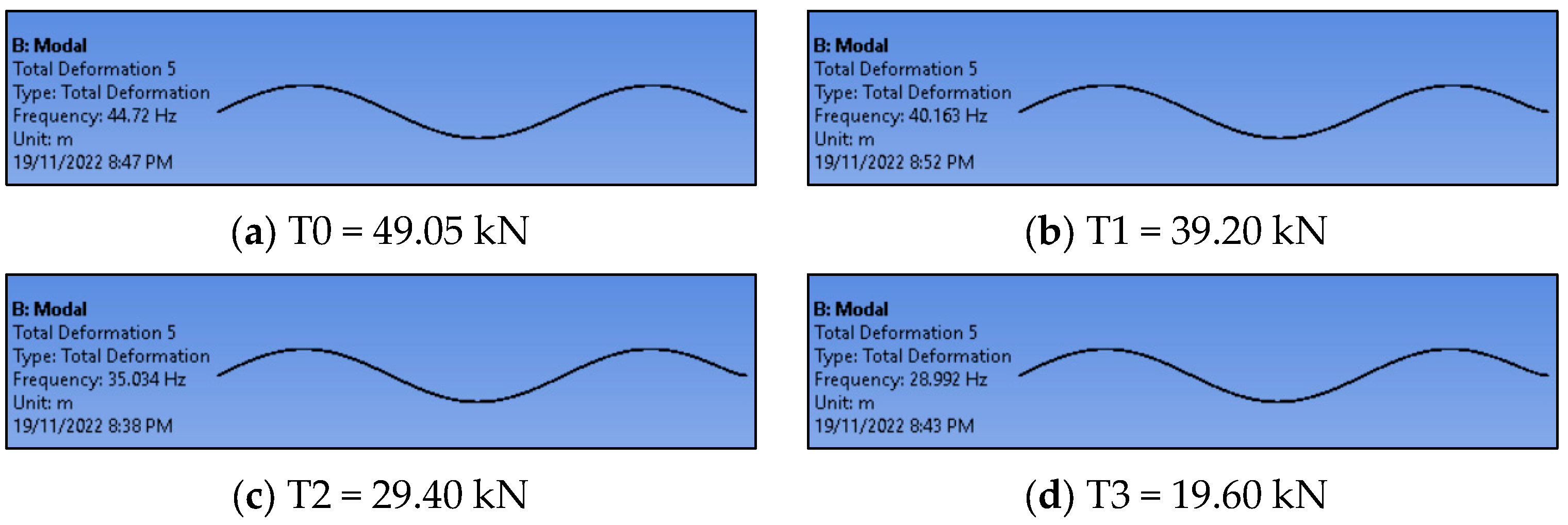
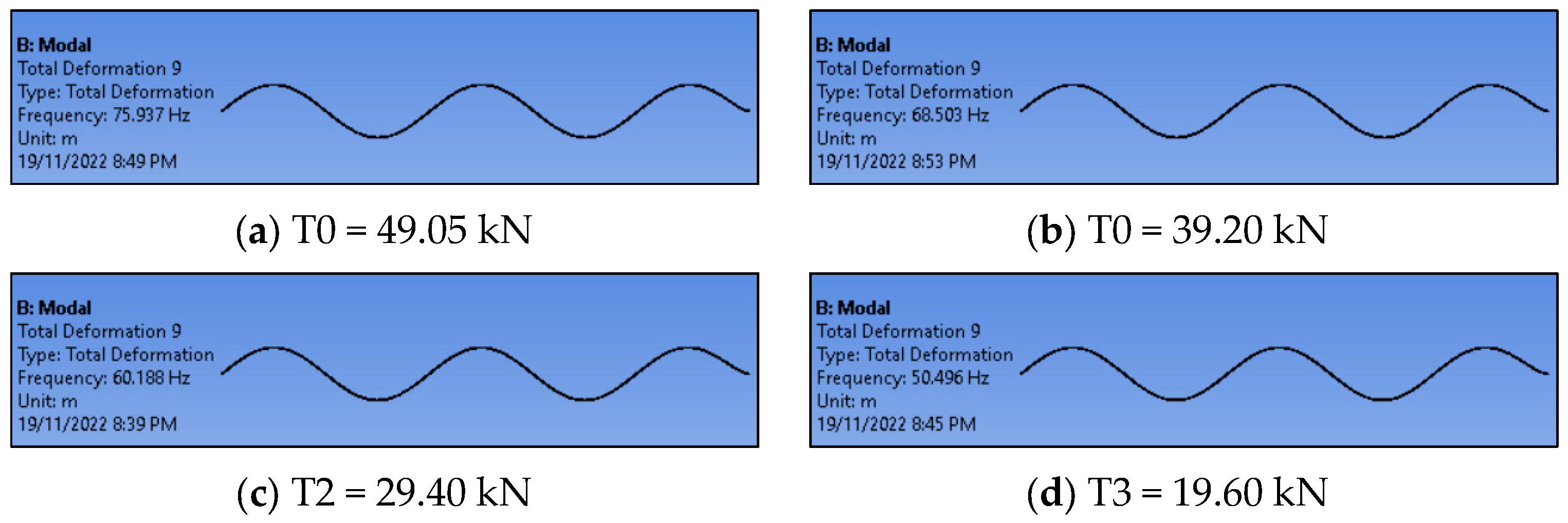
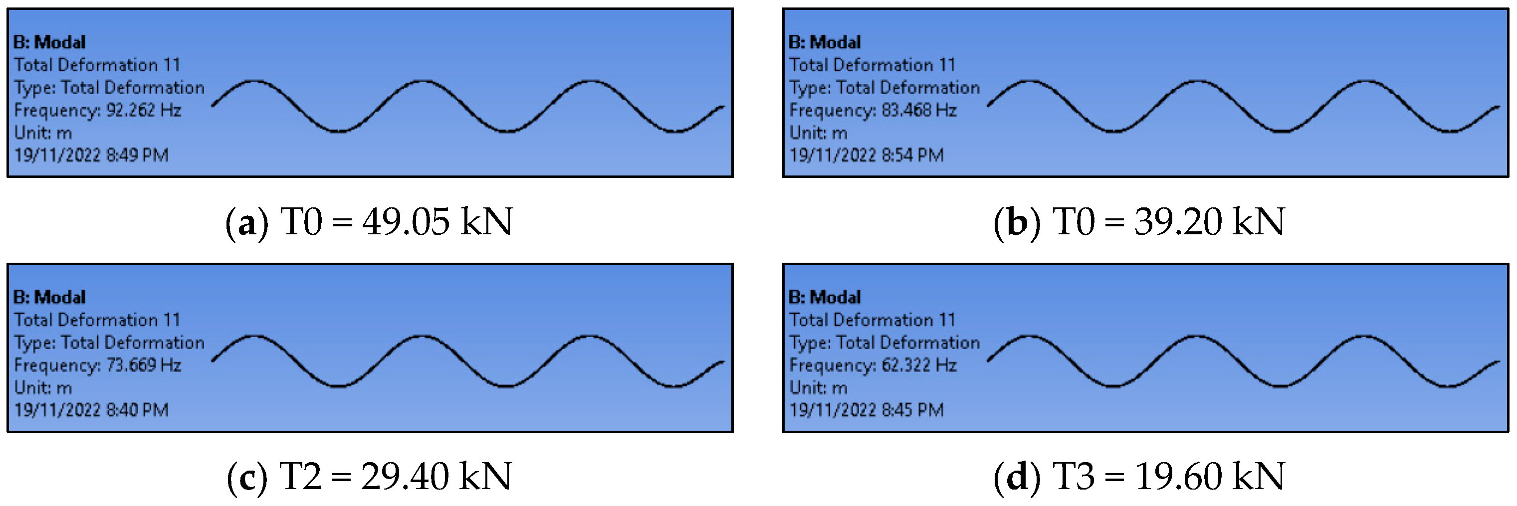
3.1. Estimation of Tension Force in Cable Structure Using the Vibration-Based Method

An external cable of a prestressed concrete girder from the experiment of Huynh and Kim (2014) [19] is employed for the vibration-based verification. It should be noted that Huynh and Kim (2014) [19] only performed experiments on the impedance of the cable. This study performs the extended numerical simulation on vibration for the cable. The cable length is 6.4 m, and the diagram is shown in Figure 7. The cable was kept by two steel bearing plates at the two ends. At the left end, the tension force was controlled and measured by a stressing jack and a load cell. At the right end, an interface with a PZT sensor was affixed to the bearing plate. At first, the cable was tensioned by the stressing jack with a tension force of 49.05 kN (i.e., case T0). For the cable tension loss scenarios, the tension force decreased gradually according to the loss extents of 20%, 40%, and 60%, which is listed in

Table 1. Cable tension loss scenarios.

Case	Loss Level (%)	Tension Force (kN)
T0	0	49.05
T1	20	39.20
T2	40	29.40
T3	60	19.60

.

In this study, the finite element model of the cable was simulated by using ANSYS software (Figure 8). In which, the steel cable was considered as an axial tensile line element with dimensions and material properties in

Table 2. Parameters of the cable.

Diameter	15.2 mm	Mass per unit length	1.37 kg/m
Elastic modulus	190 MPa	Tensile strength	260 kN
Poisson coefficient	0.3	Cross-sectional area	138.7 mm2

. For the boundary conditions, at one end of the cable, where the force tension is assigned, the horizontal and vertical displacements are restrained (the left end in Figure 8); meanwhile, the other end is restrained for horizontal, vertical, and axial displacements (the right end in Figure 8). The natural frequencies of the first six modes are presented in

Table 3. Natural frequencies versus tension forces.

Case	Loss Level (%)	Tension Force (kN)	Natural Frequency (Hz)
			${\mathsf{f}}_1$	${\mathsf{f}}_2$	${\mathsf{f}}_3$	${\mathsf{f}}_4$	${\mathsf{f}}_5$	${\mathsf{f}}_6$
T0	0	49.05	14.76	29.64	44.72	60.12	75.94	92.26
T1	20	39.20	13.23	26.58	40.16	54.1	68.5	83.47
T2	40	29.40	11.49	23.13	35.03	47.35	60.19	73.67
T3	60	19.60	9.44	19.05	28.99	39.43	50.5	62.32

. The corresponding mode shapes of the cable for four cases are illustrated from Figure 9, Figure 10, Figure 11, Figure 12, Figure 13 and Figure 14.

As shown in Figure 15, the natural frequencies decrease with decreasing in the tension force (or with increasing in the cable tension loss). The difference in natural frequencies between cable tension loss levels varies across each mode. When considering a specific level of loss, the natural frequencies of the cable demonstrate a proportional increase in relation to the modes, thereby creating a linear relationship. Based on these natural frequencies, the cable tension is determined by using Equations (2)–(8). The cable tension estimation results are listed in

Table 4. Vibration-based cable tension estimation.

Case	Loss Level (%)	Infliction (kN)	Estimation (kN)	Difference (%)
T0	0	49.05	48.73	0.66
T1	20	39.20	39.13	0.17
T2	40	29.40	29.55	0.51
T3	60	19.60	19.93	1.67

. The comparison between the estimated force and inflicted force reveals a negligible difference. This indicates that the natural frequencies obtained from the simulation are reliable. Figure 16 indicates that the estimated tension force decreases as the cable tension loss increases, demonstrating a correlation between the cable tension and the cable’s natural frequency. The estimation results are well in agreement with the experimental ones, with differences of less than 2%. The smallest difference is 0.17% for case T1, while the largest is 1.67% for case T3. Additionally, the difference between the estimation and the infliction increases with increasing the cable tension loss. In summary, the cable tension is accurately established using the vibration-based method.

3.2. Detection of Cable Tension Loss Using the Impedance-Based Method

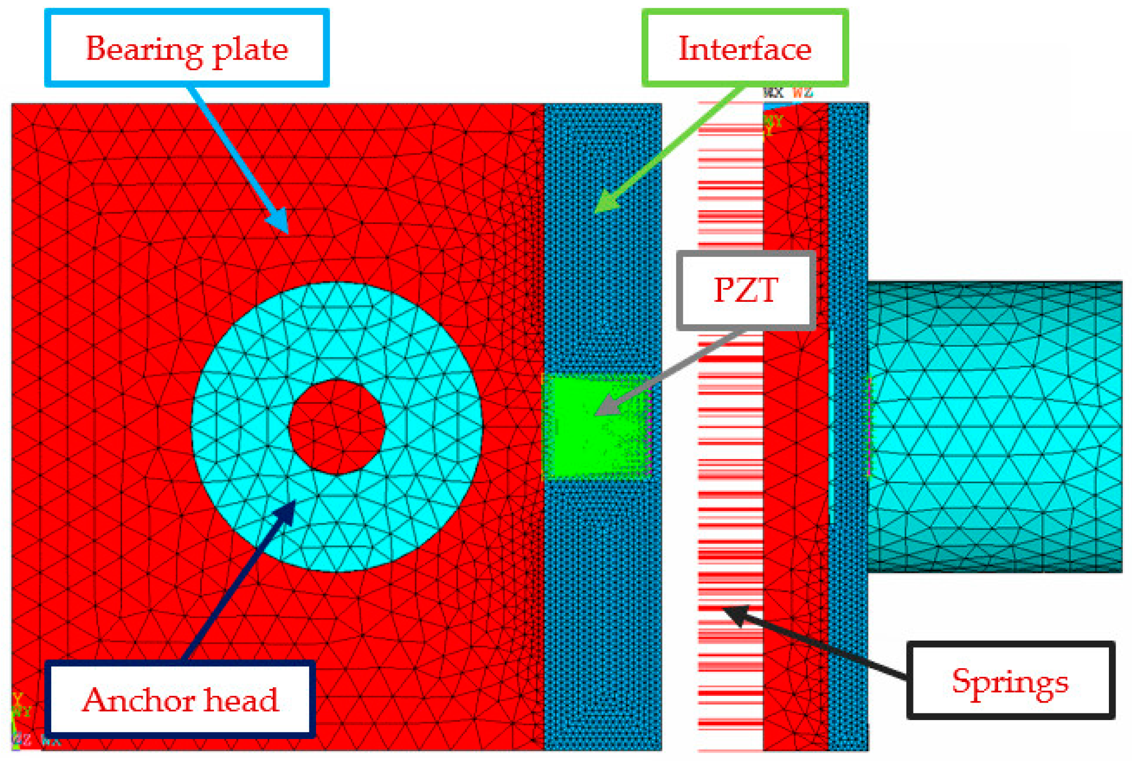
3.2.1. Cable Anchorage’s Finite Element Model

The cable tension loss was also studied by Huynh and Kim (2014) [19]. In the experiment, the impedance responses were measured for each loss level. For the cable anchorage, a 100 × 18 × 6 mm aluminum interface with a hole size of 30 × 18 × 1 mm was placed on a 100 × 100 × 10 mm steel bearing plate. A 15 × 15 × 0.51 mm PZT-5A sensor was bonded to the center of the interface’s surface. A steel anchor head fixed to the bearing plate has an outside diameter of 45 mm and an inner diameter of 15.2 mm. The tension force applied on the anchor head results in the bearing plate’s deformation. This, in turn, deformed the interface and the PZT sensor due to their near-perfect bonding with the bearing plate. The deformation caused by each tension force level was different, leading to distinct impedance responses. The impedance signatures were measured by a commercial impedance analyzer HIOKI 3532 with the frequency sweep range from 10 to 100 kHz to control the precision of impedance measurement and feature extraction. The material properties of the bearing plate, the anchor head, the interface, and the PZT-5A are presented from

Table 5. Material properties of the bearing plate and the anchor head [20].

Parameter	Symbol	Value
Elastic module	$E$	$200\times {10}^9 \mathrm{N}/{\mathrm{m}}^2$
Density	$\rho$	$7850 \mathrm{kg}/{\mathrm{m}}^3$
Poisson coefficient	$\upsilon$	0.3
Drag loss coefficient	$\eta$	0.02

,

Table 6. Material properties of the interface [20].

Parameter	Symbol	Value
Elastic module	$E$	$70\times {10}^9 \mathrm{N}/{\mathrm{m}}^2$
Density	$\rho$	$2700 \mathrm{kg}/{\mathrm{m}}^3$
Poisson coefficient	$\upsilon$	0.33
Drag loss coefficient	$\eta$	0.001

and

Table 7. Material properties of the PZT-5A sensor [20].

Parameter	Symbol	Value
Elastic deformation	$s_{ijkl}^E$ ${\mathrm{m}}^2/\mathrm{N}$	$\left(\begin{array}{c}\begin{array}{cccccc}16.4& -5.74& -7.22& 0& 0& 0\\ -5.72& 16.4& -7.22& 0& 0& 0\\ -7.22& -7.22& 18.8& 0& 0& 0\\ 0& 0& 0& 47.5& 0& 0\\ 0& 0& 0& 0& 47.5& 0\\ 0& 0& 0& 0& 0& 44.3\end{array}\end{array}\right)\times {10}^{-12}$
Dielectric coupling constant	$d_{kij}$ $\mathrm{C}/\mathrm{N}$	$\left(\begin{array}{c}\begin{array}{ccc}0& 0& -171\\ 0& 0& -171\\ 0& 0& 374\\ 0& 584& 0\\ 587& 0& 0\\ 0& 0& 0\end{array}\end{array}\right)\times {10}^{-12}$
Dielectric constant	${\epsilon }_{ijkl}^E$ $\mathrm{F}/\mathrm{m}$	$\left(\begin{array}{ccc}1730& 0& 0\\ 0& 1730& 0\\ 0& 0& 1700\end{array}\right)\times 8.854\times {10}^{-12}$
Density	$\rho$ $\mathrm{kg}/{\mathrm{m}}^3$	7750
Drag loss coefficient	$\eta$	0.0125
Dielectric loss coefficient	$\delta$	0.015

. The impedance responses within the frequency range of 10–100 kHz were measured with a frequency interval of 0.1 kHz. The impedance responses exhibited peaks in two distinct frequency domains: the first frequency domain ranging from 15–25 kHz and the second frequency domain ranging from 77–87 kHz [19].

In this study, the cable anchorage is simulated by the finite element method using ANSYS software. The three-dimensional model’s parameters are similar to the experimental ones in [19]. The model consisted of various components such as the bearing plate, the anchor head, the interface modeled using the SOLID45 element, the PZT sensor modeled by the SOLID5 element, and the springs modeled by the COMBIN14 element, as shown in

Table 8. Information of the components in the finite element model.

Component	Type	Number of Elements	Mesh Size (m)
Bearing plate	SOLID45	18,827	$5\times {10}^{-3}$
Anchor head	SOLID45	5408	$5\times {10}^{-3}$
Interface	SOLID45	73,846	${10}^{-3}$
PZT	SOLID5	225	${10}^{-3}$
Springs	COMBIN14	19,315	$3\times {10}^{-3}$

and Figure 17.

Ritdumrongkul et al. (2004) [14] investigated the changes in the cable tension with the modifications in the structural parameters at the contact surface of the bearing plate. The cable tension was replaced by the stiffness of the springs in the same direction. Therefore, this simulation model uses the horizontal springs instead of the cable tension applied to the anchor head. The spring stiffness is determined by the applied force and the corresponding displacement. In the cable anchorage model, the springs are assigned to represent the boundary conditions of the bearing plate. The bearing plate deforms under the stress when the cable is tensioned, resulting in deformation of the spring stiffness. However, the spring stiffness is an uncertain parameter when the displacement or deformation of the bearing plate is unknown during the simulation. In order to solve the problem, the trial and error method is performed to find the appropriate spring stiffness based on the cable tension applied for the lossless case (T0) and maximum loss case (T3). Then, the linear interpolation method is utilized to calculate the spring stiffness for the remaining cases (T1 and T2). The spring stiffness corresponding to the cable tension is given in

Table 9. Spring stiffness for the tension forces.

Case	Loss Level (%)	Tension (kN)	Spring Stiffness (N/m)
T0	0	49.05	$150\times {10}^6$
T1	20	39.20	$130\times {10}^6$
T2	40	29.40	$110\times {10}^6$
T3	60	19.60	$90\times {10}^6$

.

3.2.2. The Impedance Response and Damage Index

Figure 18 shows the real part of the impedance responses for the lossless case (T0). The numerical impedance response in the frequency range of 10–100 kHz is verified with the experimental one of Huynh and Kim (2014) [19]. The numerical result matches the experimental one in terms of the two impedance resonant peaks. However, due to the impact of signal disturbance during the experiment, the shapes of the two signals are minor differences. The cause of signal disturbance during the experiment is due to external influences such as the surrounding environment (temperature, wind, etc.), electro-magnetic waves, electrical wire resistances, meters and testers. Meanwhile, the cable anchorage model is simulated under ideal conditions, so there is no signal interference.

Then, to check the cable tension loss’s occurrence, the MAPD index is determined to compare cases T1, T2, and T3 with the lossless case T0. As shown in Figure 19, the MAPD index increases as the cable tension decreases. The MAPD index increases unevenly while the cable tension loss increases steadily by 20%. Thus, the MAPD index successfully warns of the cable tension loss’s occurrence; but the exact extent of the loss cannot be identified. Since the impedance responses are more complex, the linear regression or another evaluating index is employed to predict the cable tension loss’s extent. In this study, the MLP ANN is used for the cable tension prediction.

From the frequency range of 10–100 kHz, two sub-frequency domains containing the resonant peak of the impedance response are selected: the first sub-frequency range of 15–25 kHz and the second sub-frequency range of 77–87 kHz. Figure 20 and Figure 21 show the impedance responses corresponding to four cable tension cases in two sub-frequency ranges of 15–25 kHz and 77–87 kHz, respectively.

Table 10. Impedance’s peak frequencies in two frequency ranges.

Case	Loss Level (%)	Frequency Range of 15–25 kHz			Frequency Range of 77–87 kHz
		Simulation (kHz)	Experiment (kHz)	Difference (%)	Simulation (kHz)	Experiment (kHz)	Difference (%)
T0	0	19.73	19.63	0.51	82.56	82.23	0.40
T1	20	19.70	19.63	0.36	82.55	82.15	0.49
T2	40	19.65	19.57	0.41	82.54	82.03	0.62
T3	60	19.60	19.53	0.36	82.53	-	-

summarizes the resonant frequency peak of the impedance responses for the numerical simulation and the experiment. In summary, the impedance simulation results of the cable anchorage are consistent with the experimental ones. The differences between the simulation and the experiment are less than 1%. The cable anchorage model simulated by the finite element method has high reliability. Therefore, the numerical model is continued to be applied to the cable tension prediction using the MLP ANN. Impedance responses obtained from the simulation (i.e., cases T0 to T3) are used as datasets for training the MLP ANN. It should be noted that the cable tension prediction using MLP ANN is an extension of this study; it was not done in the study of Huynh and Kim (2014) [19].

4. Identification of Cable Tension Using Vibration-Based and Impedance-Based Parallel Approach

In order to identify the tension force of the cable structure and evaluate the reliability of using vibration-based and impedance-based methods in parallel, four extensive cases of the tension force applied to the cable structure are investigated as follows: VT1 = 15%, VT2 = 35%, VT3 = 55% and VT4 = 70%. It should be noted that three cases of VT1, VT2, VT3 are inside the existing cable tensions; meanwhile, the case of VT4 is outside the existing cable tensions.

4.1. Prediction of Cable Tension Using the Vibration-Based Method

The finite element model of the cable structure in Section 3.1 is used for this prediction. The cable’s natural frequencies for four extensive cases are given in

Table 11. Natural frequencies for four extensive cases.

Case	Loss Level (%)	Tension Force (kN)	Natural Frequency (Hz)
			${\mathsf{f}}_1$	${\mathsf{f}}_2$	${\mathsf{f}}_3$	${\mathsf{f}}_4$	${\mathsf{f}}_5$	${\mathsf{f}}_6$
VT1	15	41.69	13.63	27.38	41.36	55.69	70.46	85.78
VT2	35	31.88	11.96	24.05	36.40	49.15	62.40	76.27
VT3	55	22.07	10.00	20.15	30.63	41.57	53.11	65.37
VT4	70	14.72	8.22	16.64	25.44	34.80	44.88	55.80

. Then, the cable tensions are predicted by Equations (2)–(8) and are compared to the inflicted cable tension, which are illustrated in

Table 12. Cable tension for four extensive cases.

Case	Loss Level (%)	Infliction (kN)	Prediction (kN)	Difference (%)
VT1	15%	41.69	41.62	0.17
VT2	35%	31.88	32.00	0.39
VT3	55%	22.07	22.36	1.31
VT4	70%	14.72	15.10	2.61

and Figure 22. The comparison between the predicted and inflicted cable tension shows a negligible difference with an error of less than 3%. The lowest difference is 0.17% for case VT1, and the highest one is 2.61% for case VT4.

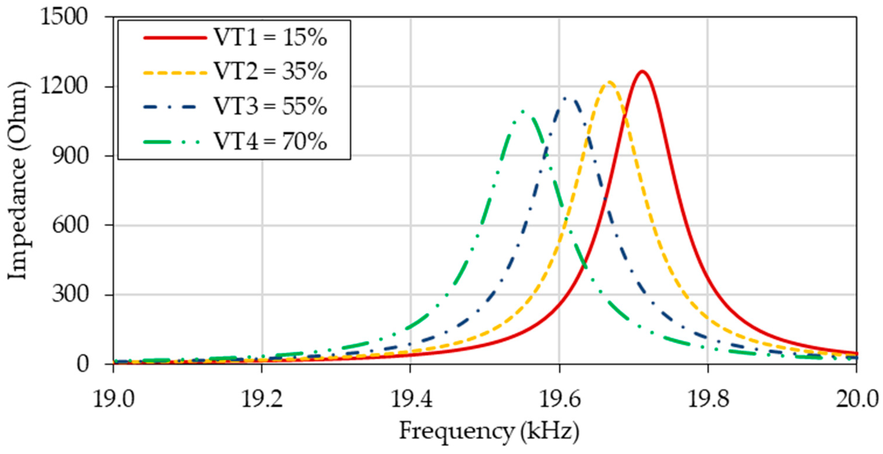
4.2. Prediction of Cable Tension Loss Using the Impedance-Based Method

As mentioned before, the change in the electro-mechanical impedance response and the MAPD index only indicate the possibility of the cable tension loss’s occurrence; however, the exact extent of the loss cannot be identified. Therefore, the MLP ANN is employed to predict the cable tension for four extensive cases. For the MLP ANN, the impedance responses in the frequency range of 19–20 kHz are selected as the datasets. The selection of this frequency range aims to reduce data and improve the prediction efficiency. Due to the impedance responses are more sensitive to the cable tension loss in the frequency range with the resonant peak.

Figure 23 shows the impedance responses obtained from the cable anchorage’s finite element model in the frequency range of 19–20 kHz for four extensive cases. The MLP ANN forward transmission neural network is constructed with four layers, including one input layer, two hidden layers (each layer has 40 neurons), and one output layer. As shown in

Table 13. Cable tension loss prediction results by MLP ANN.

Case	Data Type	Loss Level (%)	Prediction (%)					Average (%)	Error (%)
			1st	2nd	3rd	4th	5th
T0	Train	0	0.00	0.00	0.00	0.00	0.00	0.00	0.00
T1	Train	20	20.00	20.00	20.00	20.00	20.00	20.00	0.00
T2	Train	40	40.00	40.00	40.00	40.00	40.00	40.00	0.00
T3	Train	60	60.00	60.00	60.00	60.00	60.00	60.00	0.00
VT1	Predict	15	14.77	14.36	14.39	14.21	14.72	14.49	3.40
VT2	Predict	35	34.99	35.23	35.35	35.5	34.61	35.14	0.39
VT3	Predict	55	54.27	55.29	55.72	54.34	55.76	55.08	0.14
VT4	Predict	70	67.46	64.25	68.14	67.67	66.92	66.89	4.45

, the datasets of cases T1, T2, T3, and T4 are the training data; meanwhile, the datasets of cases VT1, VT2, VT3, and VT4 are the predicting data. The association weights are automatically selected and adjusted during training. In order to adjust the results of the transfer function, the bias is added for all neurons. Due to the randomness of the MLP ANN, the process is analyzed five times for each case to get the average cable tension loss prediction result. As shown in Table 13, the prediction results are high accuracy; the differences from the inflicted cable tension loss are less than 5%.

In order to investigate the influence of the frequency range selection on the cable tension loss prediction result, three frequency ranges with different widths, including 15–25 kHz, 17–22 kHz, and 19–20 kHz, are considered. The same MLP ANN training process is performed. As shown in

Table 14. Influence of frequency range on cable tension loss prediction result.

Case	Loss Level (%)	Error (%)
		15–25 kHz	17–22 kHz	19–20 kHz
VT1	15	7.07	3.31	3.40
VT2	35	2.30	0.84	0.39
VT3	55	7.11	0.24	0.14
VT4	70	22.11	7.65	4.45

, by narrowing the frequency range of the dataset, the errors of prediction results of all four loss levels are reduced. The frequency range of 19–20 kHz gives the best prediction results.

4.3. Summary

From the cable tension loss prediction by the MLP ANN in the frequency range of 19–20 kHz, the cable tensions are determined.

Table 15. Summary of cable tension results.

Case	Loss Level (%)	Infliction (kN) (1)	Vibration Method (kN) (2)	Impedance Method (kN) (3)	Difference (%) between (1) and (2)	Difference (%) between (1) and (3)
VT1	15	41.69	41.62	41.94	0.17	0.60
VT2	35	31.88	32.00	31.81	0.39	0.22
VT3	55	22.07	22.36	22.03	1.31	0.18
VT4	70	14.72	15.10	16.24	2.61	10.33

summarizes the cable tension results which are predicted by the vibration-based method and the impedance-based method in parallel. As shown in Table 15 and Figure 24, it can be seen that prediction results are highly accurate, with the errors of less than 2% for the cases of VT1, VT2, and VT3. For the case of VT4, the prediction error of the vibration-based method is 2.61%; meanwhile, the prediction error of the impedance-based method is 10.33%. As the loss level increases, the difference between the results of both methods and the inflicted value also increases. Furthermore, for the case of VT4, which is outside the training domain of the MLP ANN (i.e., 0% to 60%), the vibration-based method gives better results than the the impedance-based method. In summary, the tension forces of the cable structure are identified and confirmed when the results of the two methods in the parallel approach have low differences.

5. Conclusions

This study proposed a parallel approach of the vibration-based and impedance-based methods to identify the tension force in cable structures. The concluding remarks were drawn as follows:

(1)

The vibration and impedance responses obtained from the finite element models of the cable structure and the cable anchorage were reliable.

(2)

The identification of the cable tension using the vibration-based method gave the accurate results with the errors of less than 3%, which aligns with the experimental values.

(3)

The impedance-based method combined with the MLP ANN successfully identified the cable tension within the sub-frequency range 19–20 kHz. The impedance responses were fed into the MLP ANN to predict the cable tension with the errors of less than 2% for the cases inside the training domain, and the error of less than 11% for the case outside the training domain.

(4)

The identified tension forces of the cable structure were confirmed and concluded when the results of the two methods in the parallel approach showed the differences of less than 10%.

(5)

The simultaneous use of two techniques, including the vibration-based method and the impedance-based method, to identify the cable tension improved the reliability of the diagnostic results. Moreover, this helps to classify the damages in case the complex structures have multi-type of damages.

Future studies will explore the application of the proposed vibration-impedance parallel approach to detect the multiple structural damages. Moreover, the long-term conditions of cables may also be considered in future work, such as variations in ambient temperature, humidity, and corrosion. Additionally, we will focus on the interaction and effects of multiple damaged cables simultaneously on vibration and impedance responses.

References

1. Irvine, H.-M.; Caughey, T.-K. The linear theory of free vibrations of a suspended cable. Proc. R. Soc. Lond. 1974, 341, 299–315. [Google Scholar] [CrossRef]
2. Shinke, T.; Hironaka, K.; Zui, H.; Nishimura, H. Practical formulas for estimation of cable tension by vibration method. Proc. JSCE 1980, 294, 25–34. [Google Scholar] [CrossRef] [PubMed]
3. Shimada, T. Estimating method of cable tension from natural frequency of high mode. Proc. JSCE 1994, 50, 163–171. [Google Scholar] [CrossRef] [PubMed]
4. Zui, H.; Shinke, T.; Namita, Y. Practical formulas for estimation of cable tension by vibration method. J. Struct. Eng. 1996, 122, 651–656. [Google Scholar] [CrossRef]
5. Bhalla, S.; Soh, C. Structural impedance based damage diagnosis by piezo-transducers. Earthq. Eng. Struct. Dyn. 2003, 32, 1897–1916. [Google Scholar] [CrossRef]
6. Ren, W.-X.; Chen, G.; Hu, W.-H. Empirical formulas to determine cable tension using fundamental frequency. Struct. Eng. Mech. 2005, 20, 363–380. [Google Scholar] [CrossRef]
7. Yu, C.-P.; Hsu, K.-T.; Cheng, C.-C. Dynamic monitoring of stay cables by enhanced cable equations. Proc. SPIE 2014, 9063, 204–210. [Google Scholar] [CrossRef]
8. Hoang, N.; Nguyen, T.-N. Estimation of cable tension using measured natural frequencies. Procedia Eng. 2011, 14, 1510–1517. [Google Scholar] [CrossRef]
9. Liang, C.; Sun, F.-P.; Rogers, C.-A. Coupled electro-mechanical analysis of adaptive material systems-determination of the actuator power consumption and system energy transfer. J. Intell. Mater. Syst. Struct. 1994, 5, 12–20. [Google Scholar] [CrossRef]
10. Wang, X.-M.; Ehlers, C.; Neitzel, M. An analytical investigation of static models of piezoelectric patches attached to beams and plates. Smart Mater. Struct. 1997, 6, 204–213. [Google Scholar] [CrossRef]
11. Zagrai, A.N.; Giurgiutiu, V. Electro-mechanical impedance method for crack detection in thin plates. J. Intell. Mater. Syst. Struct. 2001, 12, 709–718. [Google Scholar] [CrossRef]
12. Ong, C.-W.; Lu, Y.; Soh, C.-K. The influence of adhesive bond on the electro-mechanical admittance response of a PZT patch coupled smart structure. In Proceedings of the Second International Conference, Singapore, 16–18 December 2002; Volume 16. [Google Scholar] [CrossRef]
13. Park, G.; Sohn, H.; Farrar, C.-R.; Inman, D.-J. Overview of piezoelectric impedance-based health monitoring and path forward. Shock. Vib. Dig. 2003, 35, 451–464. [Google Scholar] [CrossRef]
14. Ritdumrongkul, S.; Abe, M.; Fujino, Y.; Miyashita, M. Quantitative health monitoring of bolted joints using a piezoceramic actuator-sensor. Smart Mater. Struct. 2004, 13, 20. [Google Scholar] [CrossRef]
15. Kim, J.-T.; Park, J.-H.; Hong, D.-S.; Park, W.-S. Hybrid health monitoring of prestressed concrete girder bridges by sequential vibration-impedance approaches. Eng. Struct. 2010, 32, 115–128. [Google Scholar] [CrossRef]
16. Nguyen, K.-D.; Kim, J.-T. Numerical simulation of electro-mechanical impedance response in cable-anchor connection interface. J. Korean Soc. Nondestruct. Test. 2011, 30, 11–23. [Google Scholar]
17. Ho, D.-D.; Nguyen, K.-D.; Lee, P.-D.; Hong, D.-S. Wireless structural health monitoring of cable-anchorage system using vibration and impedance responses measured by smart sensors. Sens. Smart Struct. Technol. Civ. Mech. Aerosp. Syst. 2012, 8345, 255–269. [Google Scholar] [CrossRef]
18. Min, J.; Park, S.; Yun, C.-B.; Lee, C.-G.; Lee, C. Impedance-based structural health monitoring incorporating neural network techniques for identification of damage type and severity. Eng. Struct. 2012, 39, 210–220. [Google Scholar] [CrossRef]
19. Huynh, T.-C.; Kim, J.-T. Impedance-base cable force monitoring in tendon-anchorage using portable PZT-interface technique. Math. Probl. Eng. 2014, 2014, 784731. [Google Scholar] [CrossRef]
20. Huynh, T.-C.; Park, Y.-H.; Park, J.-H.; Kim, J.-T. Feasibility verification of mountable PZT-interface for impedance monitoring in tendon-anchorage. Shock. Vib. 2015, 2015, 262975. [Google Scholar] [CrossRef]
21. Huynh, T.-C.; Dang, N.-L.; Kim, J.-T. Advances and challenges in impedance-based structural health monitoring. Struct. Monit. Maint. 2017, 4, 301–329. [Google Scholar] [CrossRef]
22. Huynh, T.-C.; Ho, D.-D.; Dang, N.-L.; Kim, J.-T. Sensitivity of piezoelectric-base smart interfaces to structural damage in bolted connections. Sensors 2019, 19, 3670. [Google Scholar] [CrossRef] [PubMed]
23. Pan, W.; Li, X.; Zhu, Z.; Zhao, K.; Xie, C.; Su, Q. Detection sensitivity of input impedance to local defects in long cables. IEEE Access 2020, 8, 55702–55710. [Google Scholar] [CrossRef]
24. Fernandes, S.-R.-N.; Tsuruta, K.-M.; Rabelo, D.-S.; Finz, N.-R.-M. Impedance-based structural health monitoring applied to steel fiber-reinforced concrete structures. J. Braz. Soc. Mech. Sci. Eng. 2020, 42, 1–5. [Google Scholar] [CrossRef]
25. Huynh, T.-C.; Nguyen, T.-D.; Ho, D.-D.; Dang, N.-L.; Kim, J.-T. Sensor fault diagnosis for impedance monitoring using a piezoelectric-based smart interface technique. Sensors 2020, 20, 510. [Google Scholar] [CrossRef]
26. Dang, N.-L.; Pham, Q.-Q.; Lee, S.-Y.; Kim, J.-T. Vibration-impedance approaches for tendon monitoring in prestressed concrete structure. In Proceedings of the 2020 Structures Congress, St. Louis, MI, USA, 5–8 April 2020. [Google Scholar]
27. Nguyen, B.-P.; Tran, Q.-H.; Nguyen, T.-T.; Pradhan, A.-M.-S.; Huynh, T.-C. Understanding impedance response characteristics of a piezoelectric-based smart interface subjected to functional degradations. Complexity 2021, 2021, 5728679. [Google Scholar] [CrossRef]
28. Pham, Q.-Q.; Dang, N.-L.; Kim, J.-T. Smart PZT-embedded sensors for impedance monitoring in prestressed concrete anchorage. Sensors 2021, 21, 7918. [Google Scholar] [CrossRef]
29. Nguyen, T.-T.; Phan, T.-T.-V.; Ho, D.-D.; Pradhan, A.-M.-S.; Huynh, T.-C. Deep learning-based autonomous damage-sensitive feature extraction for impedance-based prestress monitoring. Eng. Struct. 2022, 259, 114172. [Google Scholar] [CrossRef]
30. Ho, D.-D.; Luu, T.-H.-T.; Pham, M.-N. Nondestructive crack detection in metal structures using impedance responses and artificial neural networks. Struct. Monit. Maint. 2022, 9, 221–235. [Google Scholar] [CrossRef]
Figure 1. Cable structure.
Buildings 13 02079 g001
Figure 2. Electro-mechanical interaction model between anchorage, interface, and PZT sensor.
Buildings 13 02079 g002
Figure 3. Components of the artificial neural network.
Buildings 13 02079 g003
Figure 4. General model of the MLP network.
Buildings 13 02079 g004
Figure 5. Diagram of cable tension identification using MLP ANN.
Buildings 13 02079 g005
Figure 6. Vibration-based and impedance-based parallel approach for cable tension identification.
Buildings 13 02079 g006
Figure 7. Cable structure diagram.
Buildings 13 02079 g007
Figure 8. Finite element model of the cable structure.
Buildings 13 02079 g008
Figure 9. The first-mode shape of the cable versus tension forces.
Buildings 13 02079 g009
Figure 10. The second-mode shape of the cable versus tension forces.
Buildings 13 02079 g010
Figure 11. The third-mode shape of the cable versus tension forces.
Buildings 13 02079 g011
Figure 12. The fourth-mode shape of the cable versus tension forces.
Buildings 13 02079 g012
Figure 13. The fifth-mode shape of the cable versus tension forces.
Buildings 13 02079 g013
Figure 14. The sixth-mode shape of the cable versus tension forces.
Buildings 13 02079 g014
Figure 15. The first six natural frequencies versus tension forces.
Buildings 13 02079 g015
Figure 16. Comparison of cable tension between the estimation and infliction.
Buildings 13 02079 g016
Figure 17. Cable anchorage numerical model.
Buildings 13 02079 g017
Figure 18. Impedance responses for case T0.
Buildings 13 02079 g018
Figure 19. MAPD index of impedance responses.
Buildings 13 02079 g019
Figure 20. Impedance responses in the frequency range of 15–25 kHz.
Buildings 13 02079 g020
Figure 21. Impedance responses in the frequency range of 77–87 kHz.
Buildings 13 02079 g021
Figure 22. Comparison of cable tension between the prediction and infliction.
Buildings 13 02079 g022
Figure 23. Impedance responses of four extensive cases in frequency range of 19–20 kHz.
Buildings 13 02079 g023
Figure 24. Comparison of cable tension results.
Buildings 13 02079 g024