Article

Application of Cluster Analysis to Examine the Performance of Low-Cost Volatile Organic Compound Sensors

1
Department of Civil and Mechanical Engineering, Technical University of Denmark, 2800 Kgs. Lyngby, Denmark
2
Building and Construction, Danish Technological Institute, 2630 Taastrup, Denmark
3
Department of Environmental Science, Aarhus University, 4000 Roskilde, Denmark
4
Department of Environmental and Resource Engineering, Technical University of Denmark, 2800 Kgs. Lyngby, Denmark
*
Author to whom correspondence should be addressed.
Buildings 2023, 13(8), 2070; https://doi.org/10.3390/buildings13082070
Submission received: 19 June 2023 / Revised: 8 August 2023 / Accepted: 9 August 2023 / Published: 15 August 2023
(This article belongs to the Special Issue Healthy, Digital and Sustainable Buildings and Cities)

Abstract

:
Airtight energy-efficient buildings of today need efficient ventilation to secure high indoor air quality. There is a need for affordable and reliable sensors to make demand control available in a broad range of ventilation systems. Low-cost metal oxide semiconductor (MOS) volatile organic compound (VOC) sensors offer such a possibility, but they are usually non-selective and react to broad range of compounds. The objective of the present paper was to use cluster analysis to assess the ability of five commercially available MOS VOC sensors to detect pollutants in a residential setting. We studied three scenarios: emissions from people (human bioeffluents), furnishing materials (linoleum), and human activity (surface cleaning with spray detergent). We monitored each scenario with five MOS VOC sensors and a proton-transfer-reaction–time-of-flight mass spectrometer (PTR-ToF-MS). We applied an agglomerative hierarchical clustering algorithm to evaluate the dissimilarity between clusters. Four of the five tested sensors produced signals in agreement with the concentration patterns measured with the PTR-ToF-MS; one sensor underperformed in all cases. Three sensors showed a very similar performance under all emission scenarios. The results showed that the clustering could help in understanding whether a particular sensor matched the intended emission scenario.

1. Introduction

Airtight energy-efficient buildings of today need efficient ventilation to secure high indoor air quality (IAQ). Current energy-efficient ventilation solutions frequently use the so-called demand-controlled ventilation (DCV) principle. This means that the system modulates airflows according to an immediate need expressed by different demand indicators. Those include, e.g., human presence, temperature and relative humidity, carbon dioxide (CO2) concentration, or their combinations. It is common to use the CO2 concentration as an indicator of IAQ. Yet it is often questioned whether it is sufficient, as CO2 concentration mostly represents occupant-related pollution and is valid only in the presence of building occupants. The fact that measurements of CO2 do not reveal the full picture regarding the indoor air pollution and call for other indicators has been discussed by, for example, Alonso et al. [1]. Recent advances in sensor technology have brought new types of sensors that can potentially replace or supplement CO2 sensing to control ventilation. Metal oxide semiconductor (MOS) sensors for measuring volatile organic compounds (VOC) are an example [2]. When used in DCV systems, MOS VOC sensors do not only account for air pollution related to occupancy but also for diverse events that worsen IAQ. These events comprise cleaning by means of different detergents, cooking, use of personal cosmetics, or even a sudden release of unwanted chemicals. From the IAQ viewpoint, the advantage is clear—the ventilation system increases the outdoor air supply rate when the sensor detects pollutants other than CO2. The MOS technology provides an opportunity to produce sensors that are more affordable than the state-of-the-art CO2 sensors. That is why they have become ubiquitous among so-called low-cost sensors (LCS) [3]. Other advantages of MOS sensors include a low energy consumption, small size, and high durability. As a result, residential ventilation systems can utilize DCV control strategies at a lower cost. Large commercial systems can on the other hand utilize a larger number of sensors. Such possibilities fit very well with the concept of smart ventilation [4]. MOS sensors, like the one developed by Herberger et al. [5], can integrate the measurement of human-emitted VOCs and several other typical indoor pollutants so that there is no need for a CO2 sensor. The interpretation of the signals from the low-cost sensors was extended to include the CO2 concept. Using data from a study by Burdack-Freitag et al. [6], the measured VOC signal was correlated with anthropological emissions of CO2. This resulted in the so-called CO2 equivalent concentration. The reasoning behind this cross-correlation was that the term “CO2 concentration” had become known to the public as an indicator of IAQ. As a consequence, VOC sensor signals could be more easily interpreted by building occupants.
The above-mentioned arguments speak in favor of MOS VOC sensor technology in comparison to the currently used CO2 sensors. However, there are also several research studies [3,7] stating that MOS VOC sensors suffer from several drawbacks. Authors mention cross-sensitivity to relative humidity, low resolution, and an inability to measure the concentration of individual chemicals. MOS VOC sensors react to a broad variety of compounds, which can make their application for ventilation control challenging. As DCV control was almost exclusively based on CO2 for decades [8], the amount of scientific literature related to DCV control based on VOCs or other pollutants is rather limited. Despite the limited research, a VOC-controlled DCV is being offered by an increasing number of ventilation producers. Moreover, MOS VOC sensors are frequently installed in internet-enabled indoor environmental quality monitors. These should still be considered as electronic gadgets rather than reliable monitoring instruments, but their popularity is increasing, driven by the general boom in “smart home technologies” [9]. Several studies attempted to characterize MOS VOC sensors’ performance with respect to ventilation control. However, these studies focused mostly on the consequences of the MOS VOC-based control in terms of energy efficiency or IAQ. A study conducted by Kolarik [10] showed that signals from the VOC and CO2 sensors installed in an office room agreed that ventilation was needed in the space for 49% of the occupied time, while for an additional 11% of the occupied time, only the VOC called for more ventilation. These results, together with results by Laverge et al. [11], indicate that MOS VOC sensors cannot be used directly as an alternative low-cost replacement for CO2 sensors. Field tests conducted by Merzkirch et al. [12] showed that with selection of an appropriate ventilation control strategy, application of MOS VOC sensors decreased the overall ventilation flow (or operation time) and thus led to primary energy savings while maintaining acceptable IAQ. A study by Abdul-Hamid et al. [13] demonstrated that the positioning of MOS VOC sensors in ventilated spaces plays a significant role in the achieved IAQ. A study by De Sutter et al. [14] showed a notable increase in ventilation rates (and thus energy consumption) related to the sharp peaks in the MOS VOC signals when the system used the same set point for both CO2 and MOS VOC control based on a CO2 equivalent. The use of an MOS VOC sensor will consequently result in adjustments to the ventilation strategy.
The above-mentioned practical issues regarding MOS VOC sensor performance relate to the more fundamental aspect of their performance—they react to a wide range of VOCs [15,16]. Thus, they can be considered to produce an aggregated response to the VOCs present in the air. Several studies; for example, those by Kolarik et al. [15] or Demanega et al. [17], showed that the sensor response usually strongly correlated with measurements using laboratory-grade instruments, but for many sensors, there was poor quantitative agreement. These observations were made despite the fact that the majority of producers calibrate their sensors by exposing them to single compounds (e.g., ethanol or isobutylene) or pre-defined gas mixtures [18,19]).
An objective of the present paper was to study whether several commercially available MOS VOC sensors can detect VOCs during typical residential pollution emission scenarios. The aim was to combine detailed VOC measurements using laboratory-grade instruments with data mining techniques to overcome the fact that MOS VOC sensors react to a group of compounds rather than to an individual pollutant. Our hypothesis was that it is possible to use a cluster analysis on detailed VOC data obtained by a laboratory-grade instrument together with MOS VOC signals obtained under the same experimental conditions to identify compounds with a dominant influence on the MOS VOC signals. Such performance characteristics would determine the suitability of a particular MOS VOC sensor for a concrete application.
Application of a cluster analysis using data from five commercially available MOS VOC sensors together with pollutant concentration data measured with a PTR-ToF-MS showed agreement among four sensors. Their signals appeared in the same clusters as concentration patterns of VOCs characteristic of emission scenarios of human bioeffluents, linoleum, and cleaning. One of the sensors had significantly different response patterns, thus it was not suitable to detect pollutants representing the studied scenarios. The cluster analysis seemed to be useful to identify which compounds triggered the MOS VOC sensor response in different pollution situations. However, due to the nature of the cluster analysis, we recommend analyzing the absolute concentration levels for measured pollutants at the same time. This will ensure that the analysis considers pollutants that play a realistic role in the studied exposure.

2. Materials and Methods

We created different emission scenarios corresponding to typical polluting activities in residences. We conducted all measurements in a test room that allowed for controlled ventilation and thermal environment. We conducted measurements with five commercially available MOS VOC sensors as well as with a proton-transfer-reaction–time-of-flight mass spectrometer (PTR-ToF-MS). The PTR-ToF-MS was a laboratory-grade instrument capable of measuring the real-time concentration of VOC down to ppb levels. We performed a cluster analysis on the collected data.

2.1. Selected Sensors

During the preliminary market survey, we identified seventeen commercially available MOS VOC sensors from five different producers. We limited the final selection to sensors with a delivery time of less than three months and without minimum-order-quantity restriction. This led to a choice of five sensors that were tested. Table 1 summarizes their technical parameters. The sensors coded as A, B, D, and E were available as integrated modules that enabled pre-processing of the sensor signal. This pre-processing included the built-in algorithms for conversion of the measured sensor resistance change to a signal for the equivalent concentration of total volatile organic compounds (TVOCs). For some of the sensors, the pre-processing also included proprietary auto-calibration algorithms. Such algorithms have two purposes mainly. Firstly, they deal with the cross-sensitivity of the sensor to the water vapor content in the air. Secondly, they establish a sensor’s baseline usually based on the lowest measured concentration without a change for a specific period. As the MOS VOC sensors produce relative measurements, they use the baseline to characterize “clean air”. We knew such a determination of the baseline could be problematic from an IAQ standpoint. However, the present work did not deal with this issue, and our data analysis was not sensitive to the pre-processing algorithms. While sensors A and B represented integrated modules without casing, and their practical use would require further integration on a host circuit board providing a power supply and output connectors, sensors D and E represented the “ready to use” modules that could be directly connected to building automation system. Sensor C represented solely a sensor element and provided a raw voltage signal. Sensors A and B were integrated into a commercially available indoor climate measurement device, which at the same time measured the temperature (T), humidity (RH), and CO2 concentration (CO2); for details, see Section 2.3. The device was GSM-enabled and sent data into a cloud database every 5 min. Sensors C, D, and E connected to a laboratory data logger that was capable of continuously recording the voltage signal. We did not perform any additional calibration of the sensors. For sensors A, B, and C, we checked the intra-unit consistency, which was defined as the variability between signals from individual sensors < 20% [20].

2.2. Experimental Design

We exposed the MOS VOC sensors to emission scenarios representing typical activities in residences: (1) emission of human bioeffluents, (2) emissions from furnishing materials (linoleum), and (3) emissions from house cleaning with typical detergent. Table 2 summarizes the details regarding each scenario. We tested each scenario on a separate day. Mechanical ventilation was active both during and between the experiments to eliminate the accumulation of pollution from previous experiments.
We placed the MOS VOC sensors side by side in the middle of the test room (see Section 2.3) at a height of approximately 0.85 m above the floor. We powered the sensors 48 h before the first experiment, and they remained connected to electricity during the entire experimental campaign. We placed the PTR-ToF-MS in the test room with the sampling point just beside the investigated sensors. We initiated the PTR-ToF-MS measurement approximately 30 min before the actual measurement period for each scenario to sample the background in the test room. We continued the PTR-TOF-MS measurement for several hours after the measurement period to follow the decay of the released compounds.

2.3. Experimental Facilities and Measuring Conditions

The test room was 7.0 m wide and 4.5 m deep, corresponding to a floor area of 31.5 m2; the ceiling height was 2.6 m. The outer wall of the room consisted of the building façade (concrete elements with insulation) with windows, and the opposite wall facing a hallway area consisted of glass. Painted plasterboard formed the sidewalls of the room. The floor consisted of a wall-to-wall carpet on top of a vinyl flooring. The ceiling comprised a drywall suspended ceiling system with acoustic panels and built-in lighting fixtures.
The mechanical ventilation system supplied the fresh air through two chilled beams. The system worked with an outdoor airflow rate corresponding to 0.5 h−1 in the test room. The controller adjusted the supply air temperature between 19 °C and 21 °C depending on the heat load in the test room. Five table fans ensured full mixing of the air in the test room throughout the experimental period. We used exterior perforated textile sunscreens to reduce the solar heat load on the south-facing façade. We used two thermostat-controlled electric radiators to ensure a minimum air temperature of 23 °C in the test room. We controlled the relative humidity using two ultrasonic steam humidifiers. The relative humidity set point was 50%.
We continuously measured the air temperature (accuracy: ±0.3 °C), relative humidity (accuracy: ±2%), and CO2 concentration (accuracy: ±30 ppm ± 3% of reading) in the test room. We did not conduct any measurements outside the test room. Additionally, we measured an air change rate in the test room using the decay method according to ASTM standard E741-11 [21] using tracer gas (R134a). The method provides an average air change rate over a period of 1–3 h. We used a Brüel & Kjær Photoacoustic Gas Analyzer (model 1302) to monitor the concentration of the tracer gas.

2.4. PTR-ToF-MS Measurements

We used a proton-transfer-reaction–time-of-flight mass spectrometer (PTR-ToF-MS) to measure the VOC concentrations during the emission scenarios. A PTR-ToF-MS is an analytical measurement device that allows for on-line monitoring of VOC concentrations at low detection limits with a fast response time. A PTR-ToF-MS utilizes a proton transfer reaction from H3O+ to VOC with a proton affinity higher than that of water (166.55 kcal/mol). The charged VOC molecules are then detected by a ToF mass spectrometer [22]. The PTR-ToF-MS provides an on-line quantification and, at the same time, formula confirmation of VOCs. A PTR-ToF-MS in H3O+ ionization mode does not include the detection of alkanes. Moreover, a PTR-ToF-MS does not allow distinguishing between isomers. The device has been used with success in IAQ to characterize pollution sources and map chemical reactions occurring in indoor air [23,24].
The PTR-ToF-MS 8000 (Ionicon Analytik GmbH, Innsbruck, Austria) used in the experiments was operated with hydronium ions (H3O+) as a reagent, a drift tube temperature of 70 °C, a drift pressure of 2.80 mbar, and a drift tube voltage of 650 V leading to an E/N (electric field/density of the buffer gas in the drift tube) value of around 120 Townsend (Td). Mass spectra up to m/z = 430 Da were collected at a 5 s scan rate. The instrument inlet consisted of a PEEK capillary tube heated to 70 °C and a built-in permeation unit (PerMasCal; Ionicon Analytik), which emitted 1,3-diiodobenzene used for continuous mass scale calibration. Blank measurements were obtained by coupling a charcoal filter to the instrument’s inlet tube. We processed the data generated by the PTR-ToF-MS with the software PTR-MS Viewer v. 3.2.12 (Ionicon Analytik). The PTR-MS Viewer automatically calculated the mass calibrations and the VOC mixing ratio. Compound names were assigned based on a comparison with the libraries from the PTR MS Viewer, Pagonis et al. [25] and the references therein, and a priori knowledge.

2.5. Cluster Analysis and Data Processing

We applied a clustering method to analyze the relationship between the VOC signals measured by the PTR-ToF-MS and the MOS sensors. Cluster analysis is a data mining method particularly suitable for the analysis of time series. It belongs to the data mining, pattern recognition, and statistical machine learning [26] methods. Clustering is an unsupervised data-mining method that is commonly used to discover patterns in data sets by dividing the data into several subgroups. The objective of clustering is to partition a data set into several groups with the observations in the same group as similar as possible while the observations in different groups are dissimilar to a maximum extent [27]. Clustering is commonly used to analyze time-series energy-consumption data to group similar profiles into the same subgroups and unveil the most typical load profiles. Clustering algorithms for time-series data are centroid-based methods such as k-means and k-medoids [28,29,30], hierarchical clustering with an agglomerative or divisive approach [28,30], and a self-organizing map (SOM) [31,32]. For data with a small sample size, hierarchical clustering algorithms are suitable [33].
The cloud database stored the data from sensors A and B in 5 min intervals. We downloaded the data and aggregated them with measurements of temperature, relative humidity, and CO2. Data from sensors C, D, and E were stored in a laboratory data logger every 1 min. We processed these data to obtain 5 min mean values corresponding to the time step of the data from sensors A and B. We applied the same procedure to the data from the PTR-ToF-MS collected at approximately 1 s intervals.
We applied a clustering method to an aggregated data file comprising measurements by the MOS VOC sensors and PTR-ToF-MS, temperature, relative humidity, and CO2 concentration. As the MOS VOC sensors provided a signal corresponding to a range of VOCs, their appearance in the same cluster together with specific VOCs measured by the PTR-ToF-MS would indicate their ability to detect these compounds. The statistical software R version 3.4.3 [34] was used for the analysis.
We normalized observations in the aggregated data set to avoid the influence of the absolute value of each observation. We normalized each observation against the difference of its maximum value and minimum value (the so-called min–max normalization) as shown in Equation (1):
y = ( x min x ) / ( max x min x )
where x is the observation and y is its normalized value.
As the sample size was relatively small, we decided to apply an agglomerative hierarchical clustering algorithm using the R function NbClust [35] to identify the optimal number of clusters. We compared different cluster agglomeration methods, i.e., linkage methods to measure the dissimilarity between two clusters of observations. The comparison showed that the Ward linkage method [36] was the most suitable with respect to the analyzed data. The method minimizes the total within-cluster variance as it merges the pair of clusters with the minimum between-cluster distance at each computation step. As it was unclear whether the air temperature (T) and relative humidity (RH) could be influential in the clustering results, we conducted a preliminary analysis including T and RH, excluding T, excluding RH, and excluding T and RH. The presented results describe only the final analysis of the data.

3. Results

3.1. Environmental Conditions in the Test Room

Table 3 summarizes the measurements of the air temperature, relative humidity, and air change rate. The average room temperature was about 1.7 °C higher in the case of human bioeffluent activity. The intensive internal heat loads associated with the persons who emitted bioeffluents and their personal computers were likely the cause for the elevated air temperature. The relative humidity stayed in a relatively narrow range independent of the temperature in the test room. We measured the air change rate once during the scenario involving exposure to linoleum. During scenarios in which the test room door was opened several times (human bioeffluents and cleaning), we measured the air change repeatedly.

3.2. Compounds Identified by the PTR-TOF-MS

The following section summarizes the results of measurements made with the PTR-ToF-MS. We present additional details regarding the measured compounds in Appendix B. Table 4 presents compounds measured during the human bioeffluent emission scenario. It summarizes compounds whose concentration increased more than 50% compared with the background concentration prior to occupancy. The compound names are according to the libraries from the PTR-ToF-MS software v. 3.2.12 (Ionicon Analytik), and references are listed in Table 4. Acetone and methanol accounted for the majority of the total VOC concentration. Both compounds can be associated with metabolic processes and are mainly emitted during breathing by humans [37]. Additionally, the oxidation of squalene, a compound present on human skin [38], can also produce acetone. Alkyl fragment/propyne and propanol fragment/propene constituted about 23% of the total VOC concentration. The last two compounds may originate from in-source fragmentation of longer chain alkenes. Isoprene and the acids contributed slightly above 2% to the total VOC concentration during this emission scenario.
Table 5 summarizes the compounds measured with the PTR-ToF-MS during the emission scenario with linoleum. Organic acids—from acetic and formic acid to hexanoic acid—characterized the profile of the linoleum emissions. The contribution of organic acids to the total VOCs was about 50%, and the relative contribution decreased with an increasing number of carbon atoms. The remaining part of the total concentration consisted mostly of isoprene, aldehydes, and ketones.
Table 6 gives an overview of the compounds detected with the PTR-ToF-MS during the cleaning emission scenario. The compounds we could directly relate to the use of cleaning detergent were the monoterpenes and their fragments, which increased substantially (about 20× in comparison to the background concentration prior to this emission scenario) during the cleaning activity. As is clear in Table 6, we also detected compounds related to human presence, as there was a researcher performing the cleaning in the test room. The total concentration was dominated by the bioeffluents.

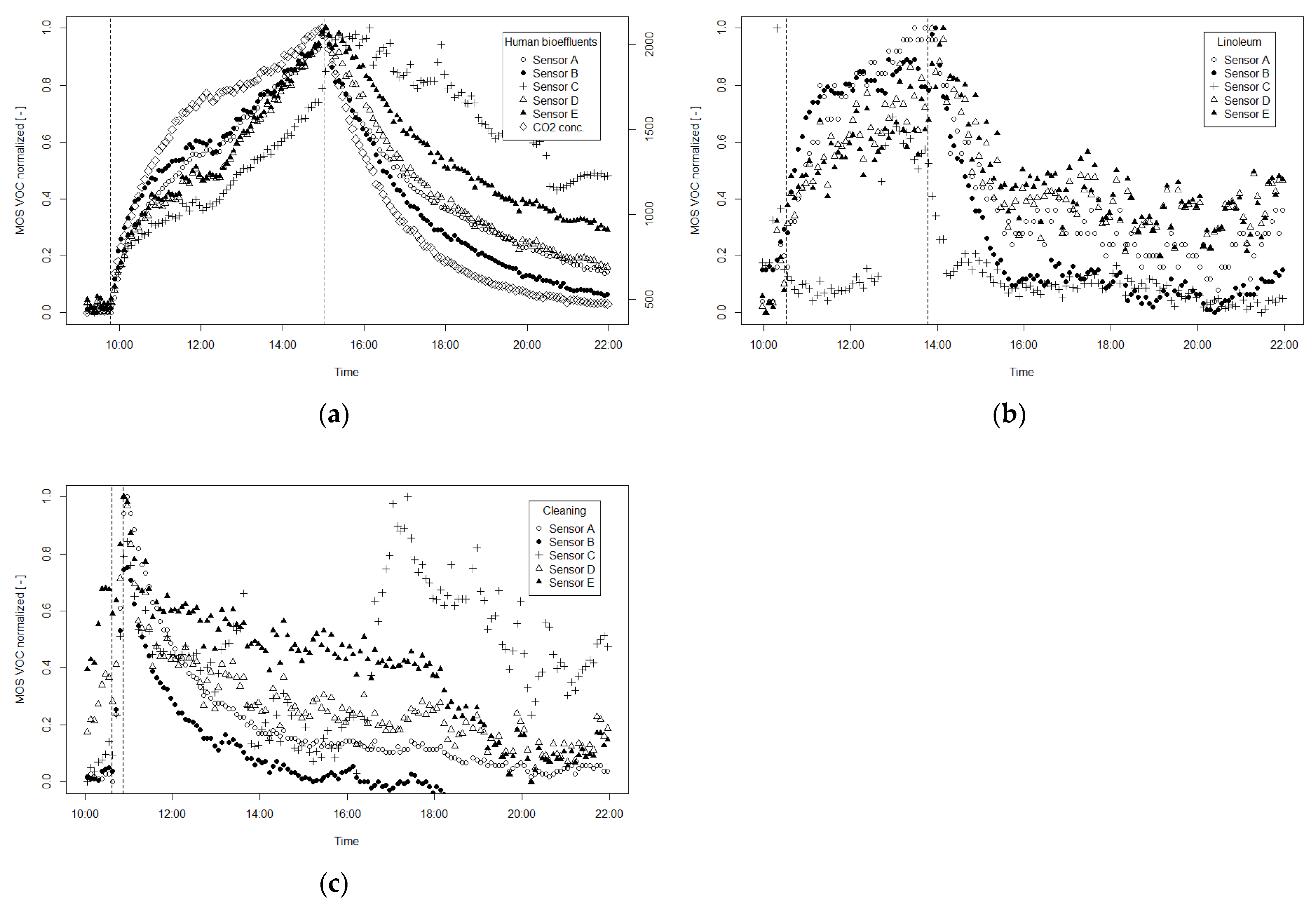
3.3. MOS VOC Sensor Signals

Figure 1 shows the normalized MOS VOC signals for the different examined emission scenarios. There were rather consistent signals from all sensors, but sensor C characterized the exposure to human bioeffluents (Figure 1a). Most of the signals followed the build-up of the human bioeffluent concentration in the test room as well as the consequent decay when persons left the test room. The signal from sensor C had somewhat the same build-up pattern, but there seemed to be a certain delay in its second part. In the decay period, the C signal was noisier, and the decay was not as obvious as it was for the remaining sensors.
For the emission scenario with linoleum (Figure 1b), the sensor signals were much more dispersed than in the case of bioeffluents, suggesting that their response to the pollutants emitted from linoleum was different. Yet, all sensors but sensor C could be characterized by immediate build-up and decay. Sensor C again underperformed, and this time it was not responsive to the pollutants emitted from linoleum (a short visit from the experimenter in the test room probably caused the peak and consequent decay in signal of sensor C during the exposure). Sensor B presented the least noisy signal.
The emission scenario with air cleaning (Figure 1c) provided a sharp response and build-up immediately after starting the cleaning. All sensors reacted to the sudden release of pollutants. After the cleaning was finished, sensors A and B presented the most consistent decays. Decays of the signals from sensors D and E were noisier, with sensor E first presenting a very shallow decay followed by a steeper decay. The signal from sensor C was rather scattered with no clear decay pattern. Moreover, there was a sudden increase in the C signal during the later period of decay.

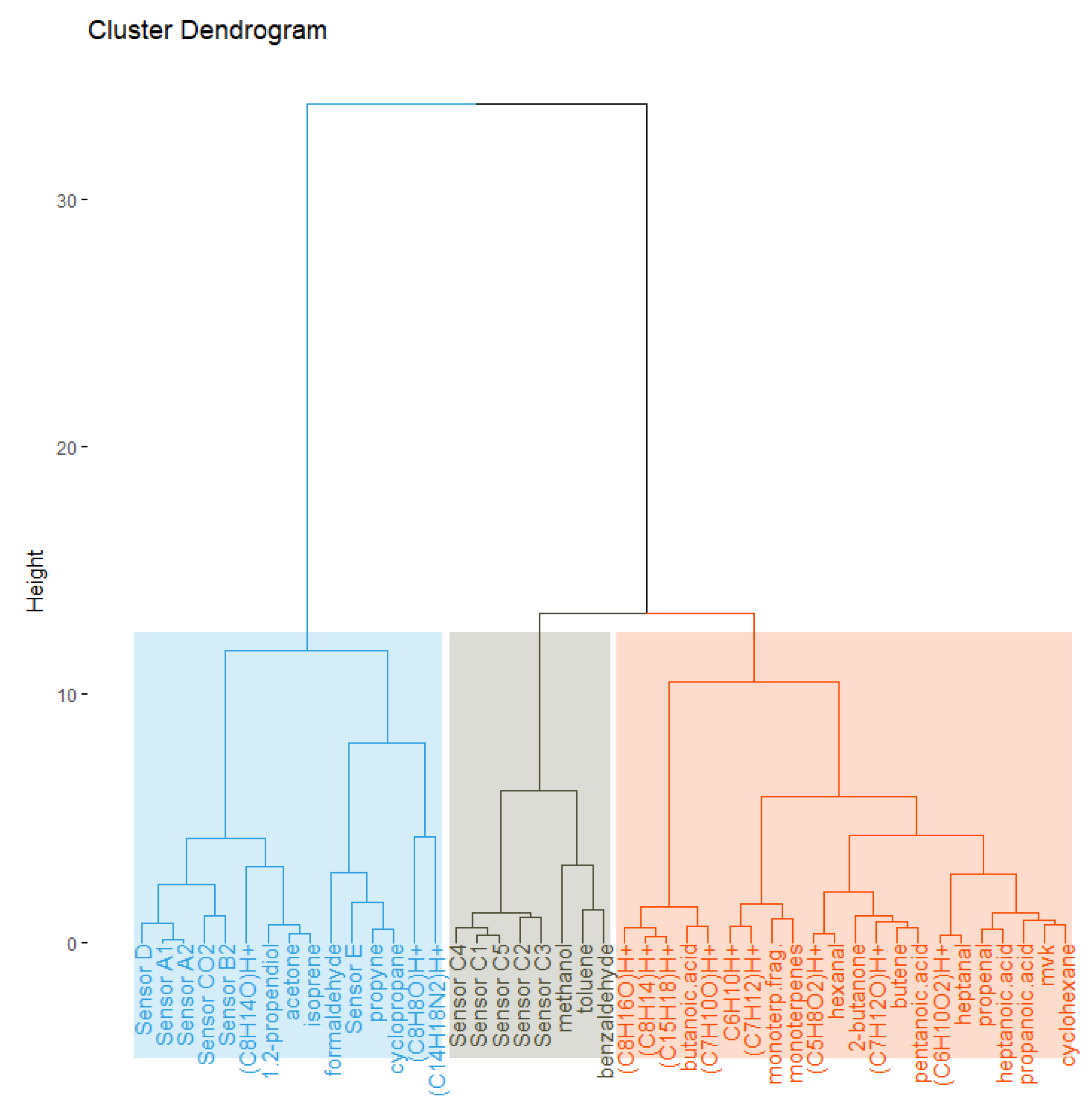
3.4. Cluster Analysis

First, we ran a cluster analysis including the T and RH signals. This preliminary analysis showed that neither the number of generated clusters nor the distribution of measured compounds and MOS VOC sensor signals changed when we added or removed the T and RH from the data set. We therefore concluded that the T and RH did not influence the clustering and excluded them from further analysis.
Figure 2 shows the results of the cluster analysis for the human bioeffluent emission scenario. The results are shown in the form of a dendrogram, which is a common practice to present clustering results displaying a close arrangement of observations with similar patterns; the colors indicate the different clusters. The dissimilarity or distance between clusters is shown as the height on the vertical axis. The data obtained during this scenario formed three clusters. The analysis placed sensors A, B, D, and E in the first cluster (marked with blue) together with compounds like acetone, isoprene, formaldehyde, and propyne (alkyl fragment; see Table 4). The second cluster (marked with a grey color) contained the signal from sensor C together with methanol, toluene, and benzaldehyde. The third and largest cluster (marked with an orange color) did not include any of the sensor signals, suggesting that the compounds identified in the orange cluster had concentration patterns that could not be associated with any signals obtained from the sensors. In other words, this result suggested that the sensors did not react to changes in concentrations for these compounds.
Dendrograms for the emission scenarios with linoleum and cleaning are presented in the Appendix A as Figure A1 and Figure A2, respectively.
The dendrogram for the emission scenario with linoleum (Figure A1) showed that the clustering divided the data into two clusters, with the signal from sensor C being the only one in the first cluster (grey). The second cluster (blue) accommodated signals from sensors A, B, D, and E as well as all compounds measured by the PTR-ToF-MS. The main compounds appearing in this cluster were acetone, ketone, and acetic acid.
The dendrogram of the clustering result for the emission scenario with cleaning (Figure A2) revealed three clusters. The first cluster (blue) accommodated all sensor signals except sensors C and E. The most important compounds in this cluster were monoterpenes, formaldehyde, and methanol. The second cluster (grey) accommodated only the signal from sensor C, as no other measured signal had a pattern similar to the sensor C response. We found the signal from sensor E in the third cluster (orange), and the other major compounds in that cluster were acetone, propene, and propyne (akryl fragment).

4. Discussion

The studied MOS VOC sensors do not offer absolute and selective measurements of individual compounds but rather an indication of the relative change in concentration of a VOC mixture. As mentioned in the Introduction, several research studies have elaborated on this matter and presented it as a main limitation of using MOS VOC sensors. In the present paper, we did not focus on the fact that MOS VOC sensors provide relative measurements and not absolute concentrations. This certainly represents a challenge when the sensors are applied for ventilation control, but sensor manufacturers deal with this issue (with variable success) by post-processing the sensor signal to establish a “clean air” baseline. However, even if they manage to tune the baseline algorithm, the problem with non-selectivity of the MOS VOC sensor remains unsolved. All reputable producers present the calibration data indicating the change in sensor signal in relation to some reference gas, usually ethanol, isobutylene, or even gas mixtures according to ISO 16000-29:2014 [19]. They conduct these tests in laboratory conditions somewhat far from the exposures in real environments.
Our approach was to mimic the realistic exposures and make a connection between the detailed analytical measurements and MOS VOC signals. We selected three emission scenarios that could be typical for residential environments but also occur frequently in commercial buildings such as schools and offices. Cluster analysis was the method used to analyze the performance of the MOS VOC sensors. Table 7 provides a general summary of the cluster analysis. The PTR-ToF-MS identified many compounds during the investigated scenarios; however, concentrations of some of them were rather low, hence their impact on the IAQ was considered negligible. As the cluster analysis used normalized data, it did not account for the absolute values of concentrations. We do not regard this as a limitation of our approach because we aimed at studying comparable concentration patterns. Including compounds at very low concentrations makes a practical interpretation of results more difficult. This is because it leads to clusters “crowded” with compounds that may have the same concentration pattern as the investigated sensors, but their actual concentrations are negligible. Consequently, in Table 7, we present only those compounds that contributed more than 5% to the total volatile organic compound (TVOC) concentration as measured by the PTR-ToF-MS (see Table 4, Table 5 and Table 6).
Table 7 reveals that sensor C performed very differently from the rest of the tested sensors. The pattern of its signal was similar to methanol in the case of the emission scenario with the human bioeffluents. In the other scenarios, the signal of sensor C could not be linked to a change in the concentration of any compound listed in Table 7. Sensor E was shown through the cluster analysis as sensitive to acetone in all three scenarios. Sensors A, B, and D had a very comparable performance under different emission scenarios if the pollutants measured were considered. The signals from sensors A, B, and D also appeared in the same cluster as the CO2 concentration in all tested scenarios. This suggests that sensors A, B, and D were responsive to pollutants whose concentration correlated with the concentration of CO2 and could be used for control in case the human bioeffluent concentration was a determining factor. In the linoleum emission scenario, all sensors but sensor C could detect emissions of organic acids that dominated the emissions related to linoleum. More tests would be necessary to clarify whether this indicates suitability to track emissions from building materials in practice or that it is a salient feature for linoleum emissions. In our experiment, the linoleum was brought into the test room on a rack. Thus, the emission characteristics were a step-change rather than a slow, continual increase, which is typical for material emissions in real buildings.
Identification of the dominant compounds that influenced the response of MOS VOC sensors was also a focus of other studies. A recent study by Schultealbert et al. [47] showed that alcohols—especially ethanol—played a major role in TVOC measurements with low-cost MOS VOC sensors. The authors concluded that these sensors need to be scientifically validated because of their broad response; which methods should be used for such validation remains a question. The methodology used in our study as well as the one used by Schultealbert et al. offer possibilities. Both require advanced laboratory-grade instrumentation.
Using the method for examining the performance of low-cost sensors presented in our paper, one could perform an evaluation of many sensors without dedicating time to their calibration. The fact that the clustering worked with normalized signals eliminates the problem of the response shift among sensors from the same producer as well as the difference in output signals among sensors from different producers (voltage, ppb TVOC, “VOC index”, etc.). Our results show that a majority of the tested sensors had a comparable performance. We could also clearly identify the sensor that did not detect the changes in IAQ at all (sensor C). As there are dozens of different MOS VOC sensors available on the market, a method allowing the screening of their basic detection capabilities seems to be necessary. Our method can be used for preliminary examination of the sensors, filtering out the sensors that underperform (in our case, it was sensor C), identifying sensors with a similar performance (in our case, these were sensors A, B, and D), and identifying sensors that specifically respond to a certain emission scenario (in our case, it was sensor E). Our method thus provides a simple yet very useful step in examining low-cost sensors before they are even examined for other features describing their performance.
Our work also had limitations. Firstly, the long-term performance of MOS VOC sensors is of high importance with respect to their suitability for ventilation control. Our experiments did not include any long-term exposures. At the same time, it is our judgement that long-term exposures would influence sensors’ drift with respect to a “clean air” baseline or a factory calibration rather than the results of the cluster analysis. Secondly, the timeline and budget of the project did not allow the repetition of pollution scenarios or testing of a higher number of sensors. Nevertheless, we consider our study robust enough to demonstrate the application of a data-clustering approach to evaluate MOS VOC performance. Further experiments should cover more sensor types as well as more emission scenarios (e.g., cooking) in residences as well as other indoor environments.

5. Conclusions

  • We used a cluster analysis to detect which of the five selected commercially available MOS VOC sensors produced signals in agreement with the concentration patterns of VOCs characteristic of three emission scenarios (human bioeffluents, cleaning, and linoleum) as measured by a laboratory-grade analytic instrument (PTR-ToF-MS).
  • Four of the five tested sensors produced signals in agreement with the concentration patterns of characteristic VOCs. One sensor underperformed in all cases and was not able to detect the characteristic concentration patterns.
  • Three sensors showed a similar performance, reacting in agreement to all emission scenarios.
  • The compounds characteristic of human presence dominated the emission scenarios with human bioeffluents and cleaning. In the cleaning emission scenario, monoterpenes and their fragments characterized the emissions from the cleaning detergent. Organic acids dominated the emissions related to linoleum.
  • We showed that a cluster analysis is a useful tool for examining the performance of low-cost MOS VOC sensors regarding their response to different emission scenarios. Consequently, even if the underlying pollutants responsible for the response are not known, the sensors that are responsive to typical pollutant generating activities can be identified. Further studies supporting this observation and advancing the method would be useful.

Author Contributions

Conceptualization, J.K., P.W., T.W. and N.L.L.; methodology, J.K., P.W., N.L.L., R.B. and R.L.; software, R.L.; investigation, J.K., N.L.L., R.B. and K.M.S.; formal analysis, J.K., R.L. and R.B.; data curation, N.L.L., R.B., R.L. and J.K.; writing—original draft preparation, J.K., R.B., N.L.L. and R.L.; writing—review and editing, P.W., K.M.S. and T.W. All authors have read and agreed to the published version of the manuscript.

Funding

This research was funded by the Danish Energy Technology Development and Demonstration Programme (EUDP; https://www.eudp.dk/en), The Danish Energy Agency, Carsten Niebuhrs Gade 43, 1577 Copenhagen, Denmark under the grant number 64016-0042.

Data Availability Statement

Not applicable.

Conflicts of Interest

The authors declare no conflict of interest.

Appendix A

Clustering dendrograms for all tested pollution scenarios.
Figure A1. Cluster dendrogram for the linoleum emission scenario. The clustering included all tested MOS VOC sensors.
Buildings 13 02070 g0a1
Figure A2. Cluster dendrogram for the cleaning emission scenario. The clustering included all tested MOS VOC sensors.
Buildings 13 02070 g0a2

Appendix B

Mass-to-charge ratios for compounds detected and identified via PTR-ToF-MS measurements in all emission scenarios.
Table A1. Mass-to-charge (m/z) ratios for compounds detected and identified via PTR-ToF-MS measurements in all emission scenarios; the compounds whose concentration increased by ≥50% compared to the background concentration are presented.
CompoundPossible Empirical FormulaDetected Ions (m/z)
FormaldehydeCH2OH+31.0178
MethanolCH4OH+33.0335
Alkyl fragment or propyneC3H4H+41.0386
AcetonitrileC2H3NH+42.0346
KeteneC2H2O43.01784
Propanol fragment (-H2O)/propene/cyclopropaneC3H6H+43.0542
AcetaldehydeC2H4OH+45.03349
Formic acidCH2O2H+47.0127
PropenalC3H4OH+57.0335
AcetoneC3H6OH+59.0491
Acetic acidC2H4O2H+61.0284
IsopreneC5H8H+69.0699
Unsaturated carbonyl (e.g., methyl vinyl ketone)C4H6OH+71.0491
Hydroxyacetone/propionic acidC3H6O2H+75.0440
1,2-PropendiolC3H8O2H+77.0597
BenzeneC6H6H+79.05423
TolueneC6H5CH379.0548
PhenolC6H6O95.04914
Monoterpene fragmentC6H8H+81.0699
cis-3-Hexen-1-ol + othersC6H10H+83.0855
Butyric acidC4H8O2H+89.0597
CyclopentylacetyleneC7H10H+95.08553
Acetylpropionyl + othersC5H8O2H+101.0597
Pentanoic acidC5H8O2H+101.0597
OctanalC7H10OH+111.0804
C7 aldehyde/ketoneC7H10OH+111.0855
1-Octen-3-ol fragment (-H2O) + others/C8-alkaneC8H14H+111.1168
Cyclohexane dionesC6H8O2H+113.0597
CycloheptanoneC7H12OH+113.0961
C6-carboxylic acid/Cyclopentane carboxylic acidC6H10O2H+115.0753
HeptanalC7H14OH+115.1117
Hexanoic acidC6H12O2H+117.0916
Anisaldehyde + othersC8H8OH+121.0670
6-Methyl-5-hepten-2-one (6-MHO)C8H14OH+127.1150
C8 saturated carbonyl + 1-octen-3-olC8H16OH+129.1295
MonoterpeneC10H16H+137.1325
NonanalC9H18O143.14360
DecanalC10H20O157.157
C12-carboxylic acidC12H22O2H+199.16953

References

  1. Jousto Alonso, M.; Wolf, S.; Jørgensen, R.B.; Madsen, H.; Mathisen, H.M. A methodology for the selection of pollutants for ensuring good indoor air quality using the de-trended cross-correlation function. Build Environ. 2022, 209, 108668. [Google Scholar] [CrossRef]
  2. Herberger, S.; Ulmer, H. Indoor Air Quality Monitoring Improving Air Quality Perception. Clean-Soil Air Water 2012, 40, 578–585. [Google Scholar] [CrossRef]
  3. Kang, Y.; Aye, L.; Ngo, T.D.; Zhou, J. Performance evaluation of low-cost air quality sensors: A review. Sci. Total Environ. 2022, 818, 151769. [Google Scholar] [CrossRef]
  4. Durier, F.; Carrié, R.; Sherman, M. What Is Smart Ventilation? Ventilation Information Paper n 38; INVIE EEIG: Brussels, Belgium, 2018. [Google Scholar]
  5. Herberger, S.; Herold, M.; Ulmer, H.; Burdack-Freitag, A.; Mayer, F. Detection of human effluents by a MOS gas sensor in correlation to VOC quantification by GC/MS. Build. Environ. 2010, 45, 2430–2439. [Google Scholar] [CrossRef]
  6. Burdack-Freitag, A.; Rampf, R.; Mayer, F.; Breuer, K. Identification of anthropogenic volatile organic compounds correlating with bad indoor air quality. In Proceedings of the 9th International Conference and Exhibition Healthy Buildings 2009, Syracuse, NY, USA, 13–17 September 2009. [Google Scholar]
  7. Won, D.Y.; Schleibinger, H. Commercial IAQ Sensors and their Performance Requirements for Demand-Controlled Ventilation; Report no. IRC-RR-323; National Research Council Canada: Ottawa, ON, Canada, 2011. [Google Scholar]
  8. Fisk, W.J.; Almeida, A.T.D. Sensor-based demand-controlled ventilation: A review. Energy Build. 1998, 29, 35–45. [Google Scholar] [CrossRef] [Green Version]
  9. Mehmet, T. A low-cost air quality monitoring system based on Internet of Things for smart homes. J. Ambient Intell. Smart Environ. 2022, 14, 351–374. [Google Scholar]
  10. Kolarik, J. CO2 Sensor versus Volatile Organic Compounds (VOC) sensor—Analysis of field measurements and implications for Demand Controlled Ventilation. In Proceedings of the Indoor Air 2014, Hong Kong, China, 7–12 July 2014. [Google Scholar]
  11. Laverge, J.; Pollet, I.; Spruytte, S.; Losfeld, F.; Vens, A. VOC or CO2: Are They Interchangeable As Sensors for Demand Control? In Proceedings of the Healthy Buildings Europe 2015, Eindhoven, The Netherlands, 18–20 May 2015. [Google Scholar]
  12. Merzkirch, A.; Maas, S.; Scholzen, F.; Waldmann, D. A semi-centralized, valve less and demand controlled ventilation system in comparison to other concepts in field tests. Build. Environ. 2015, 93, 21–26. [Google Scholar] [CrossRef]
  13. Abdul-Hamid, A.; El-Zoubi, S.; Omid, S. Evaluation of set points for moisture supply and volatile organic compounds as controlling parameters for demand controlled ventilation in multifamily houses. In Proceedings of the Indoor Air 2014, Hong Kong, China, 7–12 July 2014. [Google Scholar]
  14. De Sutter, R.; Pollet, I.; Vens, A.; Losfeld, F.; Laverge, J. TVOC concentrations measured in Belgium dwellings and their potential for DCV control. In Proceedings of the 38th AIVC Conference, Nottingham, UK, 13–14 September 2017. [Google Scholar]
  15. Kolarik, J.; Lyng, N.L.; Laverge, J. Metal Oxide Semiconductor Sensors to Measure Volatile Organic Compounds for Ventilation Control. Report from the AIVC Webinar: Using Metal Oxide Semiconductor (MOS) Sensors to Measure Volatile Organic Compounds (VOC) for Ventilation Control. Available online: https://www.aivc.org/resource/metal-oxide-semiconductor-sensors-measure-volatile-organic-compounds-ventilation-control (accessed on 13 June 2023).
  16. Collier-Oxandale, A.M.; Thorson, J.; Halliday, H.; Milford, J.; Hannigan, M. Understanding the ability of low-cost MOx sensors to quantify ambient VOCs. Atmos. Meas. Tech. 2019, 12, 1441–1460. [Google Scholar] [CrossRef] [Green Version]
  17. Demanega, I.; Mujan, I.; Singer, B.C.; Andelković, A.S.; Babich, F.; Licina, D. Performance assessment of low-cost environmental monitors and single sensors under variable indoor air quality and thermal conditions. Build. Environ. 2021, 187, 107415. [Google Scholar] [CrossRef]
  18. Fahlen, P.; Andersson, H.; Ruud, S. Sensor Tests, Demand Control Ventilation Systems; SP Report; Swedish National Testing and Research Institute: Boras, Sweden, 1992; ISBN 91-7848-331-331-X. [Google Scholar]
  19. ISO 16000-29; Indoor Air-Part 29: Test Methods for VOC Detectors. ISO: Geneva, Switzerland, 2014.
  20. Justo Alonso, M.; Madsen, H.; Liu, P.; Jørgensen, R.B.; Jørgensen, T.B.; Christiansen, E.J.; Myrvang, O.A.; Bastien, D.; Mathisen, H.M. Evaluation of low-cost formaldehyde sensors calibration. Build Environ. 2022, 222, 109380. [Google Scholar] [CrossRef]
  21. ASTM E741-11; Standard Test Method for Determining Air Change in a Single Zone by Means of a Tracer Gas Dilution. ASTM International: West Conshohocken, PA, USA, 2017.
  22. Graus, M.; Müller, M.; Hansel, A. High resolution PTR-TOF: Quantification and Formula Confirmation of VOC in Real Time. J. Am. Soc. Mass Spectrom. 2010, 21, 1037–1044. [Google Scholar] [CrossRef] [Green Version]
  23. Kolarik, B.; Wargocki, P.; Skorek-Osikowska, A.; Wisthaler, A. The effect of a photocatalytic air purifier on indoor air quality quantified using different measuring methods. Build. Environ. 2010, 45, 1434–1440. [Google Scholar] [CrossRef]
  24. Schripp, T.; Etienne, S.; Fauck, C.; Fuhrmann, F.; Märk, L.; Salthammer, T. Application of proton-transfer-reaction-mass-spectrometry for Indoor air quality research. Indoor Air 2014, 24, 178–189. [Google Scholar] [CrossRef]
  25. Jain, A.K.; Murty, M.N.; Flynn, P.J. Data clustering: A review. ACM Comput. Surv. 1996, 31, 264–323. [Google Scholar] [CrossRef]
  26. Pagonis, D.; Sekimoto, K.; de Gouw, J. A Library of Proton-Transfer Reactions of H3O+ Ions Used for Trace Gas Detection. J. Am. Soc. Mass. Spectrom. 2019, 30, 1330–1335. [Google Scholar] [CrossRef]
  27. Zhou, K.; Yang, S.; Shao, Z. Household monthly electricity consumption pattern mining: A fuzzy clustering-based model and a case study. J. Clean. Prod. 2017, 141, 900–908. [Google Scholar] [CrossRef]
  28. Jin, L.; Lee, D.; Sim, A.; Borgeson, S.; Wu, K.; Spurlock, C.A.; Todd, A. Comparison of clustering techniques for residential energy behavior using smart meter data. In Proceedings of the 31st AAAI Conference on Artificial Intelligence, San Francisco, CA, USA, 4–9 February 2017. [Google Scholar]
  29. Gianniou, P.; Liu, X.; Heller, A.; Nielsen, P.S.; Rode, C. Clustering-based analysis for residential district heating data. Energy Convers. Manag. 2018, 165, 840–850. [Google Scholar] [CrossRef]
  30. Fernandes, M.P.; Viegas, J.L.; Vieira, S.M.; Sousa, J.M.C. Segmentation of residential gas consumers using clustering analysis. Energies 2017, 10, 2047. [Google Scholar] [CrossRef] [Green Version]
  31. McLoughlin, F.; Duffy, A.; Conlon, M.A. Clustering approach to domestic electricity load profile characterisation using smart metering data. Appl. Energy 2015, 141, 190–199. [Google Scholar] [CrossRef] [Green Version]
  32. Beckel, C.; Sadamori, L.; Santini, S. Towards automatic classification of private households using electricity consumption data. In Proceedings of the BuildSys 2012—4th ACM Workshop on Embedded Systems for Energy Efficiency in Buildings, Toronto, ON, Canada, 6 November 2012. [Google Scholar]
  33. Dolnicar, S.A. Review of Unquestioned Standards in Using Cluster Analysis for Data-Driven Market Segmentation. In Proceedings of the Australian and New Zealand Marketing Academy Conference 2002, Melbourne, Australia, 2–4 December 2002. [Google Scholar]
  34. R Core Team. R: A Language and Environment for Statistical Computing. R Foundation for Statistical Computing, Vienna, Austria. Available online: https://www.R-project.org/ (accessed on 13 June 2023).
  35. Charrad, M.; Ghazzali, N.; Boiteau, V.; Niknafs, A. Nbclust: An R package for determining the relevant number of clusters in a data set. J. Stat. Softw. 2014, 61, 1–36. [Google Scholar] [CrossRef] [Green Version]
  36. Ward, J.H. Hierarchical Grouping to Optimize an Objective Function. J. Am. Stat. Assoc. 1963, 58, 236–244. [Google Scholar] [CrossRef]
  37. Fenske, J.D.; Paulson, S.E. Human breath emissions of VOCs. J. Air Waste Manag. Assoc. 1999, 49, 594–598. [Google Scholar] [CrossRef] [PubMed]
  38. Wisthaler, A.; Weschler, C.J. Reactions of ozone with human skin lipids: Sources of carbonyls, dicarbonyls, and hydroxycarbonyls. Proc. Natl. Acad. Sci. USA 2010, 107, 6568–6575. [Google Scholar] [CrossRef]
  39. Stönner, C.; Edtbauer, A.; Williams, J. Real-world volatile organic compound emission rate from seated adults and children for use in indoor air studies. Indoor Air 2018, 28, 164–172. [Google Scholar] [CrossRef] [PubMed] [Green Version]
  40. Tang, X.; Misztal, P.K.; Nazaroff, W.W.; Goldstein, A.H. Volatile organic compounds emissions from human indoors. Environ. Sci. Technol. 2016, 50, 12686–12694. [Google Scholar] [CrossRef] [Green Version]
  41. Liu, Y.; Misztal, P.K.; Xiong, J.; Tian, Y.; Arata, C.; Weber, R.J.; Nazaroff, W.W.; Goldstein, A.H. Characterizing sources and emissions of volatile organic compounds in a northern California residence using space- and time-resolved measurements. Indoor Air 2019, 29, 630–644. [Google Scholar] [CrossRef] [PubMed] [Green Version]
  42. Wilke, O.; Jann, O.; Brödner, D. VOC- and SVOC-emissions from adhesives, floor coverings and complete floor structures. Indoor Air 2004, 14, 98–107. [Google Scholar] [CrossRef]
  43. Han, K.H.; Zhang, S.; Wargocki, P.; Knudsen, H.N.; Guo, B. Determination of material emission signatures by PTR-MS and their correlation with odor assessment by human subjects. Indoor Air 2010, 20, 341–354. [Google Scholar] [CrossRef]
  44. Krejcirikova, B.; Kolarik, J.; Wargocki, P. The effects of cement-based and cement-ash-based mortar slabs on indoor air quality. Build. Environ. 2018, 135, 213–223. [Google Scholar] [CrossRef] [Green Version]
  45. Knudsen, H.N.; Clausen, P.A.; Wilkins, C.K.; Wolkoff, P. Sensory and chemical evaluation of odorous emissions from building products with and without linseed oil. Build. Environ. 2007, 42, 4059–4067. [Google Scholar] [CrossRef]
  46. Höllbacher, E.; Ters, T.; Rieder-Gradinger, C.; Srebotnik, E. Emissions of indoor air pollutants from six user scenarios in a model room. Atmos. Environ. 2017, 150, 389–394. [Google Scholar] [CrossRef]
  47. Schultealbert, C.; Baur, T.; Leidinger, M.; Conrad, T.; Amann, J.; Bur, C.; Schütze, A. Do alcohols dominate the VOC measurement of low-cost sensors? In Proceedings of the 18th Healthy Buildings Europe Conference, Aachen, Germany, 11–14 June 2023. [Google Scholar]
Figure 1. Normalized signals from five MOS VOC sensors for three emission scenarios: (a) human bioeffluents, (b) linoleum, (c) cleaning. Vertical dashed lines indicate the start (first line) and the end (second line) of the emission.
Buildings 13 02070 g001
Figure 2. Cluster dendrogram for the human bioeffluent scenario. The clustering included all tested MOS VOC sensors; “mvk” stands for unsaturated carbonyl.
Buildings 13 02070 g002
Table 1. Technical parameters of investigated sensors based on manufacturer data sheets.
AbbreviationABCDE
ConfigurationSensor moduleSensor moduleSensorSensor moduleSensor module
Output (units)TVOC eq. (ppb) 1
CO2 eq. (ppm)
TVOC eq. (ppb)
CO2 eq. (ppm)
Voltage (V)Voltage (V)Voltage (V)
Sensing rangeCO2 eqv.:
400–2000 ppm
TVOC:
0–1000 ppb
CO2 eqv.:
450–2000 ppm
TVOC:
125–600 ppb 2
NH3:
10–300 ppm 3
C6H6:
10–1000 ppm
Alcohols:
10–300 ppm
0–100% VOC0–100% VOC
Measuring accuracyN/AN/AN/A±20% of final value 5N/A
Measurement interval/response time1 s/<5 s
for TVOC
1 s/N/AN/AN/A/60 sN/A/ <13 min, <3.5 min, <1 min 6
Power supply3.3 V DC ± 5%3.3 V DC ± 0.1 V5 V DC or
AC ± 0.1 V
24 V ± 10% AC/DC24 V ± 20% AC
CommunicationI2C busI2C busanalog0–10 V or
4–20 mA
Analog: 0–10 V or 0–5 V DC
Warm up time15 min5 min>24 h1 hN/A
Operation temperature range0–50 °C0–50 °C−10–45 °C0–50 °C0–50 °C
Operation humidity range5–95%, non-condensing5–95%, non-condensing<95%N/A0–95%, non-condensing
Automatic baseline correctionYes 4YesN/AYesYes
1 Isobutylene equivalent. 2 Relative measurement; values above the defined sensing range are provided as well. 3 Calibrated using 100 ppm NH3 in clean air (T = 20 °C, RH = 65%); O2 concentration 21%. 4 The manufacturer states that no calibration is needed. 5 The manufacturer specifies that the value refers to the calibration gas, but the type of calibration gas is not specified. 6 It is possible to define the response time during installation–setup.
Table 2. Summary of emission scenarios.
ScenarioStart of PTR-ToF-MS
Measurement
Scenario StartScenario EndDescription
Human bioeffluents9:13 a.m.9:47 a.m.3:02 p.m.Six adults were seated in the test room. They were instructed not to eat spicy food or use cosmetics before the experiment. Each person was equipped with a laptop and power supply. Persons performed sedentary work corresponding to a metabolic activity of 1.2 met. Persons could drink water but not consume any food in the test room. If one of the persons needed to leave, another adult was brought in the test room as a substitute.
Linoleum9:58 a.m.10:31 a.m.1:47 p.m.Linoleum flooring was used to represent emissions from typical furnishing materials. The surface area of the linoleum was 17 m2, corresponding to half of the floor area of the test room. Linoleum strips were fixed against each other by the bottom surface so that only the upper surface of the material was exposed to air. Linoleum strips were hung on a steel rack.
Cleaning10:03 a.m.10:37 a.m.10:52 a.m.A solution consisting of 60 mL of universal citrus-scented detergent was mixed in 5 L of water as instructed by the manufacturer. Preparation of the solution took place outside the test room immediately before the activity. One adult washed all wall surfaces in the room with a cloth soaked with the solution; 240 mL of the solution was used. The cleaning took 15 min, and the remaining cleaning solution was then removed from the test room.
Table 3. Indoor environmental conditions. The values for air temperature and relative humidity represent the mean (min–max) corresponding to the period from the start of PTR-ToF-MS measurement until 10 p.m. each experimental day. The air change rate measurement was performed 1 to 3 times per activity.
ActivityTemperature (°C)
Mean (Min–Max)
Relative Air Humidity (%)
Mean (Min–Max)
Air Change Rate (h−1)
Human bioeffluents24.4 (22.6–25.7)45.5 (43.5–47.2)0.7; 0.7; 0.6
Linoleum22.8 (22.4–23.4)45.1 (43.1–46.8)0.7
Cleaning22.7 (22.3–23.0)45.1 (43.1–48.2)0.7; 0.8
Table 4. Compounds detected and identified via PTR-ToF-MS measurements during the human bioeffluent emission scenario; the compounds whose concentration increased by ≥50% compared to the background concentration are presented. The VOCs are ranked according to their contribution to the total VOC concentration. References relate to association of the compound with the studied emission scenario.
CompoundContribution to TVOCs (%)Reference
Methanol24.8[39,40]
Acetone23.1[40]
Propanol fragment (-H2O)/propene/cyclopropane12.8[40,41]
Alkyl fragment or propyne9.8[40,41]
Octanal0.9[38]
6-Methyl-5-hepten-2-one (6-MHO)3.6[38]
Formaldehyde 12.6-
Unsaturated carbonyl (e.g., methyl vinyl ketone)0.6[40,41]
Isoprene2.3[39,40]
Hydroxyacetone/propionic acid2.2[38,40,41]
1-Octen-3-ol fragment (-H2O) + others0.4[40,41]
C6-carboxylic acid0.4[40]
C8 saturated carbonyl + 1-octen-3-ol1.3[40,41]
1,2-Propendiol 10.2-
Anisaldehyde + others1.1[40,41]
Acetylpropionyl + others1.0[40,41]
cis-3-Hexen-1-ol + others1.0[40,41]
Butyric acid<0.1[40,41]
C12-carboxylic acid<0.1[40]
1 These compounds were detected during the human bioeffluent scenario, but there is no reference relating them to human presence.
Table 5. Compounds detected and identified via the PTR-ToF-MS measurements during the linoleum emission scenario; the compounds whose concentration increased by ≥50% compared to the background concentration are presented. The VOCs are ranked according to their contribution to the total VOC concentration. References relate to the association of the compound with the studied emission scenario.
CompoundContribution to TVOCs (%)Reference
Acetic acid28.0[42,43,44]
Ketene 115.3-
Formic acid13.7[44]
Acetone 113.1-
Acetaldehyde 112.8-
Propionic acid4.4[44,45]
Propenal 11.5-
Isoprene 11.4-
Butyric acid0.9[43,44]
Pentanoic acid0.6[43,44]
C8-alkane 10.3-
Cyclohexane diones 10.3-
Cyclopentane carboxylic acid 10.3-
C7 aldehyde/ketone 10.2-
Cycloheptanone 10.2-
Heptanal 10.2-
Propanol fragment (-H2O)/propene/cyclopropane 1<0.1-
Hexanoic acid<0.1[44,45]
1 These compounds were detected during the linoleum scenario, but there is no reference relating them to emission from linoleum.
Table 6. Compounds detected and identified via PTR-ToF-MS measurements during the cleaning emission scenario; the compounds whose concentration increased by ≥50% compared to the background concentration are presented. The VOCs are ranked according to their contribution to the total VOC concentration. References relate to association of the compound with the studied emission scenario.
CompoundContribution to TVOCs (%)Reference
Acetone 135.3-
Methanol 129.4-
Formaldehyde 17.7-
Propanol_fragment_(-H2O)/propene/cyclopropane 15.6-
Alkyl_fragment_or_propyne 15.5-
Monoterpene fragment4.6-
Monoterpene3.1[40,46]
Isoprene 11.6-
Cis-3-hexen-1-ol_+_others 11.3-
Toluene 21.2-
Phenol 20.9-
Acetonitrile 20.9-
Benzene 20.9-
C7H10H+ 20.8-
Nonanal 20.5-
Decanal 20.4-
1,2-propendiol0.3-
1 These compounds had a high probability of being related to the presence of a human subject conducting the cleaning in the test room; see Table 4. 2 These compounds were detected in the cleaning scenario, but there is no reference relating them to the emissions from cleaning products.
Table 7. Relations among MOS VOC sensor signals and compounds contributing > 5% to the TVOC. The signal and compound concentration profile were related if they appeared in the same cluster under a particular scenario: h—human bioeffluents; l—linoleum; c—cleaning.
Sensor ASensor BSensor CSensor DSensor E
Acetoneh/lh/l- 2h/lh/l/c
Methanolcchc-
Acetic acidll-ll
Ketenell-ll
Formic acidll-ll
Propanol fragment 1hh-hh/c
Acetaldehydell-ll
Alkyl fragment/propynehh-hh/c
Formaldehydecc-c-
CO2h/l/ch/l/c-h/l/ch/l
1 (-H2O)/propene/cyclopropane. 2 The dash indicates that the sensor and the compound never appeared in the same cluster.
Disclaimer/Publisher’s Note: The statements, opinions and data contained in all publications are solely those of the individual author(s) and contributor(s) and not of MDPI and/or the editor(s). MDPI and/or the editor(s) disclaim responsibility for any injury to people or property resulting from any ideas, methods, instructions or products referred to in the content.

