Estimating the Concrete Ultimate Strength Using a Hybridized Neural Machine Learning

Abstract

Concrete is a highly regarded construction material due to many advantages such as versatility, durability, fire resistance, and strength. Hence, having a prediction of the compressive strength of concrete (CSC) can be highly beneficial. The new generation of machine learning models has provided capable solutions to concrete-related simulations. This paper deals with predicting the CSC using a novel metaheuristic search scheme, namely the slime mold algorithm (SMA). The SMA retrofits an artificial neural network (ANN) to predict the CSC by incorporating the effect of mixture ingredients and curing age. The optimal configuration of the algorithm trained the ANN by taking the information of 824 specimens. The measured root mean square error (RMSE = 7.3831) and the Pearson correlation coefficient (R = 0.8937) indicated the excellent capability of the SMA in the assigned task. The same accuracy indicators (i.e., the RMSE of 8.1321 and R = 0.8902) revealed the competency of the developed SMA-ANN in predicting the CSC for 206 stranger specimens. In addition, the used method outperformed two benchmark algorithms of Henry gas solubility optimization (HGSO) and Harris hawks optimization (HHO) in both training and testing phases. The findings of this research pointed out the applicability of the SMA-ANN as a new substitute to burdensome laboratory tests for CSC estimation. Moreover, the provided solution is compared to some previous studies, and it is shown that the SMA-ANN enjoys higher accuracy. Therefore, an explicit mathematical formula is developed from this model to provide a convenient CSC predictive formula.

1. Introduction

In recent years, the world of engineering has witnessed significant developments that have enabled experts to solve problems with higher accuracy and convenience [1,2,3]. These developments include a wide range of civil engineering domains such as geotechnical [4,5] and water [6,7] analysis. Focusing on the structural aspects of this field, engineers have benefitted from various technologies and simulation tools for analyzing the behavior of structures (and their particular elements) [8,9,10] under different loading conditions [11,12,13].

Also, many laboratory tools and innovative approaches have been successfully employed for investigating the behavior of structural materials [14,15,16]. When it comes to construction materials, concrete is known as one of the most effective ones. Mechanical parameters, and particularly the compressive strength of concrete (CSC), play an appreciable role in determining the quality of this popular material [17,18]. Since the non-linear effect of different parameters should be incorporated for CSC analysis, machine learning models, and more particularly artificial neural networks (ANN), have been regarded for this aim. Some of the primary efforts in utilizing the ANNs for the CSC problem can be found in studies like [19,20]. Prasad et al. [21] used this model for predicting the CSC of self-compacting and high-performance concretes containing high-volume fly ash. Duan et al. [22] successfully modeled the CSC of recycled aggregate concrete using ANNs. Regarding the 99.55% correlation, as well as the mean absolute percentage error (MAPE) below 2%, they concluded the applicability of the ANN. Naderpour et al. [23] applied a similar methodology to environmentally friendly concrete. ANNs have also performed profitably for other properties of concrete like slump [24], creep and shrinkage [25], and strain [26].

In a more general sense, many scientific efforts have been dedicated to foreseeing a specific behavior, particularly prediction tasks [27,28,29]. As for the application of machine learning models for CSC modeling, many attempts can be found in the published literature [30,31,32]. Akande et al. [33] introduced support vector machine (SVM) as a stable approach for this objective. Also, the proposed SVM outperformed the ANN with respect to root mean square error (RMSE) values (23.14 vs. 27.15). Feng et al. [34] used an adaptive boosting algorithm (a combination of several learners) to predict the CSC. While the mean absolute percentage error (MAPE) for this model was around 6.8%, conventional benchmarks including ANN and SVM achieved MAPE of around 10 and 15%, respectively. Accordingly, the suggested model presented a promising approximation of the CSC. The authors also showed that specifying 80% of the data for pattern recognition leads to an acceptable accuracy. Moreover, scholars like Başyigit et al. [35] and Vakhshouri and Nejadi [36] proved the feasibility of fuzzy-based tools for handling the CSC estimation.

Moreover, optimization algorithms have served as prominent techniques for analyzing mechanical parameters of concrete such as CSC. Kandiri et al. [37] optimized an ANN by a multi-objective slap swarm algorithm for the prediction of CSC when the mixture contains ground granulated blast furnace slag. The authors compared the accuracy of the developed models with a well-known machine learning tool called the M5P model tree. The larger MAPE of the MP5 (12.05 vs. 7.25%) demonstrated the superiority of the optimal ANN. Naseri et al. [38] attained an optimal design of sustainable concrete by predicting the CSC using a potent metaheuristic algorithm called water cycle algorithm (WCA). In addition to the WCA, popular algorithms like ANN and SVM were also considered. The most sustainable mixtures were eventually detected among the 16 tested ones. Moreover, the cuckoo search algorithm (CSA) was used for a similar purpose by Boindala and Arunachalam [39]. As another usage of the WCA, Ashrafian et al. [40] coupled multivariate adaptive regression splines (MARS) with this technique to create a capable hybrid model. Similar to earlier efforts, the authors also proved the superiority of the developed model over a number of conventional tools like standard MARS and ANN. Grey wolf optimizer (GWO) is another well-known metaheuristic approach that was used by Golafshani et al. [41] for hybridizing the ANN and ANFIS toward simulating the CSC. In research by Zhang et al. [42], beetle antennae search (BAS) was employed to tune the parameters of a random forest model. The resultant hybrid method was applied to estimate the uniaxial CSC of concrete containing oil palm shell. Regarding the 96% correlation observed for the prediction phase, the developed BAS-based ensemble was introduced as an efficient approximator. Likewise, Akbarzadeh et al. [43] professed the outstanding accuracy of ANN tuned by electromagnetic field optimization (EFO) for predicting the CSC. The EFO algorithm outperformed several compatible techniques including sine cosine algorithm (SCA) and cuttlefish optimization algorithm (CFOA). This study presented the final solution in the form of a complex mathematical formula for convenient estimations of CSC. Further attempts concerning the use of metaheuristic algorithms for modeling different concrete characteristics can be found in studies [44,45,46,47].

As reported by the literature review, metaheuristic integrated approaches show high promise for studying CSC prediction. On the other hand, many old and reputable optimizers such as ICA [48], PSO [49], whale optimization algorithm [50], etc., have gained sufficient attention for this purpose. Therefore, due to the continuous development of metaheuristic algorithms, recent studies have mainly focused on evaluating newly devised techniques to keep the existing solutions updated. Some examples of these new metaheuristic algorithms that are coupled with ANN for CSC prediction are multi-tracker optimization algorithm (MTOA) [51], satin bowerbird optimizer (SBO) [52], equilibrium optimizer (EO) [53], beetle antennae search (BAS) [54], etc. Each of these algorithms follows a specific search scheme in order to find the optimum contribution between the CSC and concrete mixture components. Slime mold algorithm (SMA) [55] is another capable metaheuristic algorithm that has not been investigated in previous studies. This work presents various configurations of this algorithm that rules an ANN to attain an optimum non-linear prediction of the CSC. Moreover, two other metaheuristic algorithms of Harris hawks optimization (HHO) [56] and Henry gas solubility optimization (HGSO) [57] are employed as benchmark techniques to comparatively validate the performance of the SMA. The HHO and HGSO are also among newly developed techniques, and using them would add new insights to the body of knowledge regarding predicting mechanical properties of concrete, particularly the CSC. The final solution of this research is translated into a monolithic mathematical formula in order to provide a convenient predictive approach for the users.

2. Materials and Methods

2.1. Data and Statistics

It Yeh [19] collected the information (i.e., the conditions and results) of 1030 typical compressive strength tests (on the cylinder specimens with height 15 cm) to create the dataset used for capturing and reproducing the CSC behavior in this work. This dataset can be accessed at http://archive.ics.uci.edu/ml/datasets/Concrete+Compressive+Strength (accessed on 12 June 2021).

The amount of each ingredient of the specimen mixtures is considered as a separate independent factor for the corresponding CSC. Figure 1 shows the values of (a) cement, (b) blast furnace slag (BFS), (c) fly ash (FA1), (d) water, (e) superplasticizer (SP), (f) coarse aggregate (CA), (g) fine aggregate (FA2), and (h) age. The values of the mentioned factors are in the ranges of [102.00, 540.00], [0.00, 359.40], [0.00, 200.10], [121.75, 247.00], [0.00, 32.20], [801.00, 1145.00], [594.00, 992.60], and [1.00, 365.00], respectively. Meanwhile, the obtained CSCs are shown in Figure 1i with the minimum and maximum values of 2.33 to 82.60.

Table 1. Information on some training and testing specimens.

Inputs								Target	Group
Cement (kg/m3)	BFS (kg/m3)	FA1 (kg/m3)	Water (kg/m3)	SP (kg/m3)	CA (kg/m3)	FA2 (kg/m3)	Age (day)	CSC (MPa)
149.00	236.00	0.00	176.00	13.00	847.00	893.00	28.00	32.96	Training
375.00	0.00	0.00	186.00	0.00	1038.00	758.00	7.00	26.06	Testing
213.76	98.06	24.52	181.74	6.65	1066.00	785.52	56.00	47.13	Testing
310.00	0.00	0.00	192.00	0.00	971.00	850.60	3.00	9.87	Training
290.35	0.00	96.18	168.08	9.41	961.18	865.00	100.00	48.97	Testing
277.00	117.00	91.00	191.00	7.00	946.00	666.00	28.00	43.57	Training
190.00	190.00	0.00	228.00	0.00	932.00	670.00	365.00	53.69	Training
446.00	24.00	79.00	162.00	11.64	967.00	712.00	3.00	25.02	Testing
236.00	157.00	0.00	192.00	0.00	972.60	749.10	28.00	32.88	Testing
214.90	53.80	121.89	155.63	9.61	1014.30	780.58	3.00	18.02	Training
330.50	169.60	0.00	194.90	8.10	811.00	802.30	28.00	56.62	Testing
181.38	0.00	167.01	169.59	7.56	1055.60	777.80	56.00	35.57	Training
475.00	118.80	0.00	181.10	8.90	852.10	781.50	91.00	74.19	Training
213.72	98.05	24.51	181.71	6.86	1065.80	785.38	100.00	53.90	Testing
218.23	54.64	123.78	140.75	11.91	1075.70	792.67	3.00	27.42	Training
300.00	0.00	0.00	184.00	0.00	1075.00	795.00	7.00	15.58	Testing
480.00	0.00	0.00	192.00	0.00	936.20	712.20	28.00	43.94	Testing
134.70	0.00	165.70	180.20	10.00	961.00	804.90	28.00	13.29	Training
397.00	0.00	0.00	185.00	0.00	1040.00	734.00	28.00	39.09	Training
218.23	54.64	123.78	140.75	11.91	1075.70	792.67	14.00	35.96	Testing

provides some examples of the used data. As is seen, each row is labeled as either “Training” or “Testing”. It determines the group that this data lies in. Based on random selection, as well as the division ratio of 80:20, a total of 824 and 206 samples form the training and testing datasets, respectively.

2.2. Methodology

Figure 2 shows the graphical methodology of the present study. The first section describes data provision, followed by the model development and prediction stage, and accuracy assessment. In the end, a comparison is carried out among the models to extract the formula from the outstanding one.

2.2.1. The SMA Algorithm

The name slime mold (SM) refers to Physarum polycephalum [58] that inhibits cool and humid areas. The main inspiration of the SMA algorithm is the dynamic nutritional behavior of the SM called Plasmodium. This stage includes three steps that an organic matter performs for seeking food, surrounding the discovered food, and secreting enzymes to digest it. Figure 3 shows the foraging morphology that forms an interconnected venous network using multiple food blocks at the same time.

Inspired by the explained foraging behavior, Li, Chen, Wang, Heidari and Mirjalili [55] developed the SMA as a novel optimization approach. The objective of the SM is to find the optimal path to the largest concentration of nutrients [59]. Although the most promising food source is regarded by the SM, it needs to consider two important factors in foraging, namely speed and risk. Selecting the appropriate time for leaving the searched area (toward a new one) is another challenge for the SM. To figure it out, the algorithm uses heuristic or empirical rules. However, as explained, the algorithm can simultaneously exploit more than one source [60]. Overall, when several food sources with different qualities are at their disposal, an adaptive search strategy is executed to attain the best one.

Mathematically, the SMA comprises four major stages that are described below.

(a)

Approaching food: Regarding the odor in the air, the SM approaches food based on the below equation:

$$\overrightarrow{X\left(t+1\right)}=\left\{\begin{array}{c}\overrightarrow{X_b\left(t\right)}+\overrightarrow{vb}·\left(\overrightarrow{W}·\overrightarrow{X_A\left(t\right)}-\overrightarrow{X_B\left(t\right)}\right), r<p\\ \overrightarrow{vc}·\overrightarrow{X\left(t\right)}, r\ge p\end{array}\right.,$$

(1)

where$t$signifies the current iteration, $\overrightarrow{vc}$ follows a linear decrease from 1 to 0, $\overrightarrow{vb}$ is a parameter ranging in $\left[-a,a\right]$ where $a=\mathrm{arctanh}\left(-\left(\frac{t}{\max \_t}\right)+1\right)$, and $\overrightarrow{W}$ stands for the weight of the SM. Also, locations belonging to the SM, the individual with the largest odor concentration so far, and two randomly selected individuals are represented by $\overrightarrow{X}$, $\overrightarrow{X_b}$, $\overrightarrow{X_A}$ and $\overrightarrow{X_B}$, respectively. Moreover, given $S\left(i\right)$ as the fitness of $\overrightarrow{X}$ and $DF$ as the best fitness obtained ever, the term $p$ can be formulated as follows:

$$p=\mathit{tanh}\left|S\left(i\right)-DF\right| i\in 1,2,\dots ,n.$$

(2)

Equation (3) provides $\overrightarrow{W}$.

$$\overrightarrow{W\left(SmellIndex\left(i\right)\right)}=\left\{\begin{array}{c}1+r·\log \left(\frac{bF-S\left(i\right)}{bF-wF}+1\right), condition \\ 1-r·\log \left(\frac{bF-S\left(i\right)}{bF-wF}+1\right), others\end{array}\right.,$$

(3)

$$SmellIndex=sort\left(S\right),$$

(4)

where $condition$refers to ranking the first half of the population with respect to $S\left(i\right)$. The term $r$ is a random number in $\left[0,1\right]$, $bF$ and $wF$ stand for the optimal and worst finesses grasped in the current repetitions, respectively, $SmellIndex$ provides the ascending sequence of sorted $S\left(i\right)$s.

(b)

Wrapping the food: This stage models how the venous tissue structure of the SM is contracted during the search. In this regard, three parameters including the power of the waves released by the bio-oscillator, the thickness of the vein, and the speed of the cytoplasm flows are directly proportional to the concentration level of the food contacted by the vein. As explained, the SMA prioritizes different food blocks based on their concentrations. The regions with larger concentrations receive larger weights and vice versa. Thus, the position of the SM is updated toward better regions. This process is formulated in Equation (5),

$$\overrightarrow{X^{\ast }}=\left\{\begin{array}{c}rand·\left(UB-LB\right)+LB,rand<z \\ \overrightarrow{X_b\left(t\right)}+\overrightarrow{vb}·\left(W·\overrightarrow{X_A\left(t\right)}-\overrightarrow{X_B\left(t\right)}\right),r<p \\ \overrightarrow{vc}·\overrightarrow{X\left(t\right)}, r\ge p \end{array},\right.$$

(5)

in which $LB$ and $UB$ are the lower and upper bounds, and $rand$and $r$stand for the random value between 0 and 1.

(c)

Grabbling the food: The cytoplasmic flow in the veins is affected by the waves released by the biological oscillator. To simulate the variations of the SM’s venous width, three vectors of $\overrightarrow{vc}$, $\overrightarrow{vb}$, and $\overrightarrow{W}$ are considered. $\overrightarrow{W}$ provides a mathematical presentation of the SM’s oscillation frequency at different food concentrations. This parameter helps the SM to achieve a better food source by accelerating its movement toward high-quality ones and vice versa. The $\overrightarrow{vb}$ value randomly ranges in $\left[-a,a\right]$ and it heads to 0 as the number of iterations increases. The $\overrightarrow{vc}$ value ranges in [−1, 1] and finally reaches 0. During this stage, some organic members are assigned to explore the remaining areas even if the SM reaches a more potential source compared to earlier attempts. It enables the algorithm to seek a better food block all over the area. Notably, the SM decides whether to select the proposed food source or look for another one with respect to the oscillation of $\overrightarrow{vb}$.

The Pseudo-code of the SMA is presented as Algorithm 1.

Algorithm 1. Pseudo-code of SMA [55].

$$\begin{gathered} \mathrm{Initialize}\mathrm{the}\mathrm{parameters}\mathit{popsize}Max\_iteraition; \\ \mathrm{Initialize}\mathrm{the}\mathrm{positions}\mathrm{of}\mathrm{slime}\mathrm{mould}{X}_i\left(i=1,2,\dots ,n\right); \\ \mathbf{While}(t\le Max\_iteraition) \\ \hspace{1em}\mathrm{Calculate}\mathrm{the}\mathrm{fitness}\mathrm{of}\mathrm{all}\mathrm{slime}\mathrm{mould}; \\ Update bestFitness, X_b \\ \hspace{1em}\mathrm{Calculate}\mathrm{the}W\mathrm{by}\mathbf{Equation}\left(3\right); \\ \hspace{1em}\mathbf{For}each search portion \\ \hspace{1em}Update p,vb, vc; \\ \hspace{1em}Update positions by Equation \left(5\right); \\ \hspace{1em}\mathbf{End}For \\ \hspace{1em}t=t+1; \\ \mathbf{End}\mathbf{While} \\ \mathbf{Return}bestFitness, X_b; \end{gathered}$$

(d)

Computational complexity analysis: Considering different steps of the SMA (i.e., initialization, assessing the fitness, sorting, updating the weights, and updating the locations), the complexity of the algorithm is explained in this section. Let N and T be the number of the SM’s cells and the maximum number of iterations, respectively, in a D-dimensional space. Then, O(N), O(N + N log N), O(N × D), and O(N × D) are the computational complexity of initialization, fitness evaluation and sorting, weight update, and location update, respectively. Hence, the overall complexity of the SMA can be expressed as O(N ∗ (1 + T ∗ N ∗ (1 + log N + 2 ∗ D))) [55].

2.2.2. Benchmark Trainers

Inspired by Henry’s law, the HGSO is one of the most recent metaheuristic algorithms. It was developed by Hashim, Houssein, Mabrouk, Al-Atabany and Mirjalili [57]. A modified version was also designed by Hashim et al. [61]. Also, the HGSO was used by Cao et al. [62] for optimizing the parameters of a regression SVM model. In this algorithm, the position and a so-called characteristic “partial pressure” are initially assigned to each gas. The gases are then clusterized into a number of groups. The identification of the best gases is then carried out. Based on the specific rules of the algorithm, the position and solubility of each gas are updated toward raising the quality of the solution. It is worth noting that updating the worst particles is also considered as a measure for escaping from the local optimum. The algorithm is mathematically detailed in relevant studies like [63,64]:

The second benchmark algorithm is the HHO that was designed by Heidari, Mirjalili, Faris, Aljarah, Mafarja and Chen [56]. The HHO has shown high applicability for various complex problems like analyzing landslide susceptibility [65] and slope stability [66]. The basis of this algorithm is the cooperative interaction between Harris’ hawks for a shocking hunt that comprises tracing, encircling, approaching, and attacking. These steps are devised in three major stages. The first one is named exploration dedicated to seeking and discovering the prey. The two next stages are based on the energy of the prey. After transforming from exploration to exploitation, the attacking measures are taken in the exploitation stage. For more explanations about the HHO, please refer to [67,68].

2.3. Accuracy Indicators

To assess the performance of the developed models, two error indicators of RMSE and mean absolute error (MAE) are used. In addition, the Pearson correlation coefficient (R) is defined to reflect the agreement between the products of the networks with target values. This index can be in a range of [−1, +1]. Taking K as the number of data and $CS{C}_{i_{observed}}$ and $CS{C}_{i_{predicted}}$ as the expected and modeled CSC, respectively, Equations (6)–(8) formulate the RMSE, MAE, and R.

$$RMSE=\sqrt{\frac{1}{K}{{\displaystyle \sum _{i=1}^K[(CS{C}_{i_{observed}}-CS{C}_{i_{predicted}})]}}^2},$$

(6)

$$MAE=\frac{1}{K}{\displaystyle \sum _{I=1}^K|CS{C}_{i_{observed}}-CS{C}_{i_{predicted}}|},$$

(7)

$$R=\frac{{\displaystyle \sum _{i=1}^K(CS{C}_{i_{predicted}}-{\overline{CSC}}_{predicted})(CS{C}_{i_{observed}}-{\overline{CSC}}_{observed})}}{\sqrt{{\displaystyle \sum _{i=1}^K{(CS{C}_{i_{predicted}}-{\overline{CSC}}_{predicted})}^2}}\sqrt{{\displaystyle \sum _{i=1}^K{(CS{C}_{i_{observed}}-{\overline{CSC}}_{observed})}^2}}}.$$

(8)

3. Results and Discussion

3.1. Model Configuration and Training

In this work, the efficiency of the SMA scheme for the CSC modeling is examined. As explained, this algorithm plays the role of a trainer for an ANN processor. Composed of eight, seven, and one neuron(s) in the input, hidden, and output layers, respectively, a three-layer multi-layer perceptron (MLP) [69] serves as the ANN used for being hybridized by the SMA. The topology of the used ANN is obtained after trying various cases and it is presented in Figure 4. In order to form the problem function, the proposed ANN is represented by its mathematical form where it is fed by training samples. In the neurons of the hidden layer, the inputs are received from the former layer, and weight is determined for each one. The neuron then adds a bias to the value resulting from this multiplication [70]. The activation function is a significant element of the ANNs that is eventually applied to the calculations of each neuron to release the main response. In this work, Tansig and Purelin are considered the activation functions of the hidden and output layers, respectively.

Like other metaheuristic algorithms, the SMA tries to augment a random candidate solution during the implementation. It is fulfilled by an iterative procedure until either the desired goodness or the maximum number of iterations is satisfied. Figure 5 shows that each population size of the SMA has minimized the objective function (training RMSE in this case) in predicting the CSC. For this research, the values of the objective function (on the y-axis) reflect the RMSE of training in each iteration. Noticing the initial and final objective function values, this figure shows that the SMA algorithm has great potential in reducing the error of ANN training.

Table 2. Optimal RMSEs obtained for the tested configurations.

Algorithm	Population Size
	10	25	50	75	100	200	300	400	500
SMA	8.7830	8.1813	8.4056	7.9688	8.2738	8.0212	8.1812	7.3831	7.4055
HGSO	12.8753	11.0752	11.7703	11.4388	11.4658	9.0477	10.4068	11.0786	10.1627
HHO	11.6988	11.1059	11.4161	11.1815	10.7291	10.4342	10.7521	10.2017	10.4970

provides the latest RMSEs of the tested configurations of the SMA. The same trial and error were performed for the HGSO and HHO as well. According to this table, although the final RMSEs of all population sizes are close, the differences can still reflect the eminent effect of population size. The best response of SMA, HGSO, and HHO algorithms is obtained for the population size of 400, 200, and 400, respectively. These configurations are selected to represent the SMA-ANN, HGSO-ANN, and HHO-ANN in the subsequent sections.

3.2. Accuracy Assessment

It was mentioned that the learning process was based on the training data. It means that the RMSEs reported in the previous section correspond to the training results. Thus, the proposed SMA-ANN achieved an RMSE of 7.3831 in grasping the CSC behavior. Also, the MAE was 5.7885. Figure 6 shows the histogram chart of the errors in this phase. The word error refers to the simple difference between the $CS{C}_{i_{observed}}$ and $CS{C}_{i_{predicted}}$ for each of the 824 data. In Figure 6, it can be seen that the error values follow a normal distribution, meaning that the higher the error magnitude, the lower the frequency. In general, this indicates desirable prediction results for all used models.

The RMSE and MAE for the benchmark models indicate a lower quality of training for the ANNs trained by the HGSO (9.0477 and 7.1566, respectively) and HHO (10.2017 and 8.2355). Since the training error represents tuning the weights and biases of the ANN, it can be deduced that the SMA algorithm found a more suitable matrix of these parameters.

Figure 7 shows the correlation charts of the training results. Visually, it is seen that all three charts show an acceptable correlation for the used models. However, the products of the SMA-ANN are in better agreement with the ideal situation (line Y = T). Also, the calculated R indices indicate an 89.37%, an 84.42%, and a 78.46% agreement between the expected CSCs and those estimated by the SMA-ANN, HGSO-ANN, and HHO-ANN.

The CSC pattern derived in the training phase was used to predict the CSC for 206 samples considered for evaluating the generalizability of the mapped relationship. A comparison of the modeled CSC with the estimated values is shown in Figure 8. This figure illustrates that all three models have shown good sensitivity to the changes and fluctuations in the CSC pattern.

With an RMSE of 8.1321, as well as an MAE of 6.1361, the SMA-ANN could reproduce the CSC with a good level of accuracy. Similar to the training phase, the proposed model achieved a larger accuracy in comparison with the benchmarks of the HGSO-ANN (RMSE = 9.9893 and MAE = 7.6427) and the HHO-ANN (RMSE = 11.5099 and MAE = 9.1671). Moreover, an agreement was observed between the training and testing results, meaning the better the model is trained, the more accurate outputs it produces.

Testing outputs are also depicted versus the expected CSCs in the form of correlation charts in Figure 9. Referring to the chart of the SMA-ANN, it can be said that this model can present a reliable prediction of the CSC for stranger conditions. In other words, the captured pattern is properly generalized to testing data. The calculated Rs for the models were 0.8902, 0.8278, and 0.7583, which demonstrates the superiority of the SMA over both HGSO and HHO.

Assessing the training and testing results together, it can be concluded that the used metaheuristic algorithms (i.e., SMA, HGSO, and HHO) performed suitable optimizations for adjusting the weights and biases of the ANN during the training process. These optimized parameters were used to create potential ANNs that could reliably predict the CSC.

3.3. A CSC Formula

As discussed, the better performance of the SMA points out the higher capability of this search scheme in tuning the ANN parameters including connecting weights and the bias of each neuron (Figure 4). The process by which the SMA-ANN estimates the CSC is summarized in Equation (9). It indicates applying the weights (i.e., [LW]) and bias (i.e., [b2]) of the output neuron to the response coming from hidden neurons. Likewise, this response is produced via multiplying the inputs (i.e., [I]) by the corresponding weights (i.e., [IW]) added to the bias vector (i.e., [b2]) and eventually applying $Tansig \left(x\right)=\frac{2}{1+e^{-2x}}-1$ as the activation function.

CSC = [LW] * (Tansig (([IW] * [I]) + [b1])) + [b2].

(9)

The terms used in the above equation are acquired based on

Table 3. The parameters of the predictive formula in Equation (9).

Parameter	Value
$IW$	$\left[\begin{array}{cccccccc}0.1381& -0.5092& 0.7425& 0.9454& 0.9959& 0.0459& -0.2287& 0.6467\\ -0.1934& -1.1992& -0.8799& -0.1856& -0.0123& 0.3267& 0.1319& -0.8830\\ -0.1269& 0.1029& -1.0653& 0.0773& -0.5025& -0.8111& -1.0077& 0.3078\\ -0.7477& -0.5067& 0.4525& -0.3054& -0.8152& 0.8423& -0.6242& 0.5573\\ 0.1034& 0.8107& 0.4600& -0.0100& -0.8089& 1.1472& 0.4757& -0.3344\\ 0.7039& 0.9927& 0.1850& 0.0316& -0.0522& 0.8930& -0.8899& -0.2825\\ -0.1854& 0.9990& 0.6670& -0.2774& -0.2457& -0.5999& 0.6380& -0.8981\end{array}\right]$
$I$	$\left[\begin{array}{c}Cement\\ BFS\\ FA1\\ water\\ SP\\ CA\\ FA2\\ Age\end{array}\right]$
$b1$	$\left[\begin{array}{c}-1.7855\\ 1.1903\\ 0.5952\\ 0.0000\\ 0.5952\\ 1.1903\\ -1.7855\end{array}\right]$
$LW$	$\left[\begin{array}{ccccccc}0.4433& 0.7756& 0.4244& 0.8918& -0.9618& 0.0239& -0.4702\end{array}\right]$
$b2$	$\left[\begin{array}{c}0.7595\end{array}\right]$

:

3.4. Importance Analysis

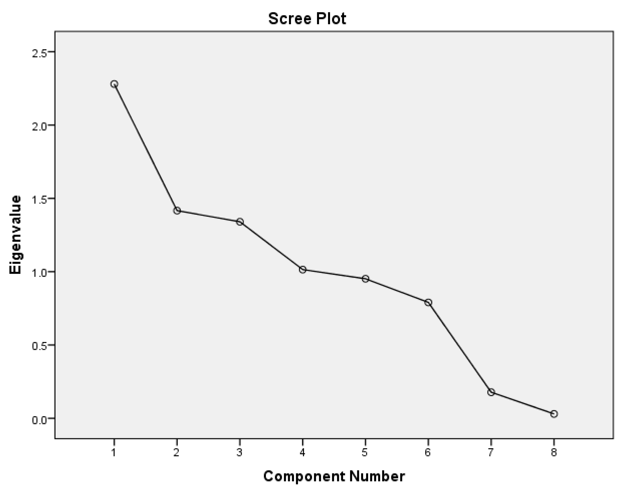
Owing to the fact that there are various influential parameters for determining the CSC [71,72,73], analyzing the importance of the input parameters is a significant step, especially when it comes to machine learning applications. To attain it, the principal component analysis (PCA) technique [74] is used within the IBM SPSS Statistics 22 environment. This technique creates some components, each representing an independent combination of the existing inputs. An eigenvalue is calculated for each component, and if the eigenvalue exceeds the threshold = 1, it means that the corresponding component is significant [75]. Figure 10 shows the calculated eigenvalues.

According to this figure, four components acquired eigenvalues > 1. Based on further statistics, these four components account for an around 75.6% variation in the dataset.

Table 4. Rotated component matrix obtained from varimax rotation method (loading factors lower than −0.75 and greater than +0.75 are shown with red and blue colors, respectively).

Inputs	Component
	1	2	3	4
Cement	0.084	0.940	0.196	0.047
BFS	0.033	−0.076	−0.922	0.234
FA1	0.269	−0.662	0.384	0.032
Water	−0.878	−0.016	−0.247	0.056
SP	0.781	−0.003	0.094	0.391
CA	0.028	−0.041	0.152	−0.939
FA2	0.334	−0.265	0.470	0.342
Age	−0.613	0.168	0.257	0.205

presents the rotated component matrix, giving details of these components obtained from the varimax rotation method. Based on the earlier literature, two thresholds of +0.75 and −0.75 can be considered for identifying the most significant inputs [76,77]. Therefore, the inputs with loading factors lower than −0.75 and greater than +0.75 are shown with red and blue colors, respectively. Eventually, it is found that the PCA analysis suggests Cement, BFS, Water, SP, and CA as the most important inputs.

3.5. Further Discussion and Future Studies

The models that were suggested in this work could achieve a reliable early analysis of the CSC based on the effects of mixture characteristics including cement, BFS, FA1, water, SP, CA, FA2, and age. However, it is worth discussing that the suggested model, i.e., the SMA-ANN, has achieved significant improvements with respect to some of the previous studies [43,52,53,54].

Table 5. Comparing accuracy indices with some previous studies.

Study	CSC Range (Mpa)	Model	RMSE	MAE	Correlation (R & R2)
This study	[2.33, 82.60]	SMA-ANN	8.1321	6.1361	0.89028
[52]	[4.23, 96.30]	ANN-HGSO	9.5248	7.8632	0.87394
		ANN-SFO	8.5728	7.0550	0.87936
[43]	[2.33, 82.60]	ANN-SCA	10.0340	7.8248	0.80249
		ANN-CFOA	9.8392	7.6538	0.79832
[53]	[2.33, 82.60]	BP–MLP (Single ANN)	8.2675	6.2103	0.788
[54]	[2.33, 82.60]	BP–MLP (Single ANN)	8.9753	6.8112	0.7442
		SCE–MLP	8.3540	6.4657	0.7876

compares the accuracy indices of this study to those that were commonly used in the cited studies. The respective RMSE and MAE of the SAM-ANN were 8.1321 and 6.1361, which are comparably smaller than those in the mentioned studies. Likewise, the R index was 0.89028, which is higher than the corresponding correlation indices in previous studies. This comparison indicates that the SMA-ANN outperformed several single and optimized versions of the ANN model. In other words, the results of this study add a capable methodology to the field of CSC prediction.

Nowadays, concrete is being used in many parts of the construction industry [78,79,80]. Hereupon, it is important to exploit efficient ways towards practical usage of the suggested models. In this sense, it can be explained that these models provide reliable, non-destructive, and cost-efficient approaches for predicting the CSC which is a non-linear and complex mechanical parameter of concrete. Engineers may use intelligent models in order to achieve a reliable design of the concrete mixture with respect to the desired CSC. Another application can be evaluating the sensitivity of the CSC to a specific mixture ingredient. For instance, engineers may be interested in assessing the variation of CSC with the changes in cement characteristics. Also, the results of the PCA analysis can be considered for this purpose, because this analysis revealed that Cement, BFS, Water, SP, and CA have the greatest influence on the CSC. To sum up, since the behavior of the CSC has been nicely understood by the models, they are applicable to predict this parameter for various mixtures without the need for conducting destructive and time-consuming laboratory tests.

Notwithstanding the advancement achieved in this study, there are some limitations that can be considered for conducting future studies. For instance, the proposed methodologies (i.e., SMA, HHO, and HGSO) can be compared to newer metaheuristic algorithms for further improving the solution. Another idea can be applying the results of the PCA analysis to reduce the dimension of the problem. More clearly, since the used dataset consists of a large number of inputs, reducing them can result in a less complicated ANN network, and enhance the prediction efficiency. Based on the PCA results, future studies are recommended to predict the CSC by considering the effect of Cement, BFS, Water, SP, and CA and disregarding FA1, FA2, and Age of the mixture. The results then can be compared to those of the present study to determine whether this idea can improve the accuracy of prediction.

4. Conclusions

In this work, a novel search method based on the foraging actions of slime mold was tested for training a popular neural system applied to the prediction of concrete compressive strength. The SMA trained an 8 × 7 × 1 MLP neural network by relating the CSC to eight influential factors. The results were evaluated for the training and testing phases using three accuracy indicators. The obtained RMSEs (7.3831 and 8.1321, 9.0477 and 9.9893, and 10.2017 and 11.5099 for the training and testing phases of the SMA-ANN, HGSO-ANN, and HHO-ANN, respectively) demonstrated the superiority of the proposed technique over two recently developed colleagues in both grasping and reproducing the CSC behavior. The above 89% correlation between the expected and estimated CSCs showed that the SMA-ANN can be a promising predictive model for practical applications. Comparison with the literature disclosed the higher accuracy of the suggested SMA-ANN against some previously used models. The final solution was translated into a mathematical format to provide a reliable and convenient formula for predicting the CSC. Moreover, the PCA importance assessment revealed that Cement, BFS, Water, SP, and CA are the most important ingredients of the concrete for predicting the CSC. In the end, some ideas were suggested to cope with the limitations of the study in future projects.

References

- Wang, J.; Tian, J.; Zhang, X.; Yang, B.; Liu, S.; Yin, L.; Zheng, W. Control of time delay force feedback teleoperation system with finite time convergence. Front. Neurorobotics 2022, 16, 877069. [Google Scholar] [CrossRef]
- Ban, Y.; Liu, M.; Wu, P.; Yang, B.; Liu, S.; Yin, L.; Zheng, W. Depth estimation method for monocular camera defocus images in microscopic scenes. Electronics 2022, 11, 2012. [Google Scholar] [CrossRef]
- Gu, Q.; Tian, J.; Yang, B.; Liu, M.; Gu, B.; Yin, Z.; Yin, L.; Zheng, W. A novel architecture of a six degrees of freedom parallel platform. Electronics 2023, 12, 1774. [Google Scholar] [CrossRef]
- Zhang, C.; Yin, Y.; Yan, H.; Zhu, S.; Li, B.; Hou, X.; Yang, Y. Centrifuge modeling of multi-row stabilizing piles reinforced reservoir landslide with different row spacings. Landslides 2023, 20, 559–577. [Google Scholar] [CrossRef]
- Zhou, S.; Lu, C.; Zhu, X.; Li, F. Preparation and characterization of high-strength geopolymer based on BH-1 lunar soil simulant with low alkali content. Engineering 2021, 7, 1631–1645. [Google Scholar] [CrossRef]
- Jia, S.; Dai, Z.; Zhou, Z.; Ling, H.; Yang, Z.; Qi, L.; Wang, Z.; Zhang, X.; Thanh, H.V.; Soltanian, M.R. Upscaling dispersivity for conservative solute transport in naturally fractured media. Water Res. 2023, 235, 119844. [Google Scholar] [CrossRef]
- Zhou, J.; Wang, L.; Zhong, X.; Yao, T.; Qi, J.; Wang, Y.; Xue, Y. Quantifying the major drivers for the expanding lakes in the interior Tibetan Plateau. Sci. Bull 2022, 67, 474–478. [Google Scholar] [CrossRef]
- Pishro, A.A.; Zhang, Z.; Pishro, M.A.; Xiong, F.; Zhang, L.; Yang, Q.; Matlan, S.J. UHPC-PINN-parallel micro element system for the local bond stress–slip model subjected to monotonic loading. In Structures; Elsevier: Amsterdam, The Netherlands, 2022; pp. 570–597. [Google Scholar]
- Hong, Y.; Yao, M.; Wang, L. A multi-axial bounding surface py model with application in analyzing pile responses under multi-directional lateral cycling. Comput. Geotech. 2023, 157, 105301. [Google Scholar] [CrossRef]
- Huang, H.; Li, M.; Yuan, Y.; Bai, H. Theoretical analysis on the lateral drift of precast concrete frame with replaceable artificial controllable plastic hinges. J. Build. Eng. 2022, 62, 105386. [Google Scholar] [CrossRef]
- Huang, H.; Yuan, Y.; Zhang, W.; Li, M. Seismic behavior of a replaceable artificial controllable plastic hinge for precast concrete beam-column joint. Eng. Struct. 2021, 245, 112848. [Google Scholar] [CrossRef]
- Ghasemi, M.; Zhang, C.; Khorshidi, H.; Zhu, L.; Hsiao, P.-C. Seismic upgrading of existing RC frames with displacement-restraint cable bracing. Eng. Struct. 2023, 282, 115764. [Google Scholar] [CrossRef]
- Xia, Y.; Shi, M.; Zhang, C.; Wang, C.; Sang, X.; Liu, R.; Zhao, P.; An, G.; Fang, H. Analysis of flexural failure mechanism of ultraviolet cured-in-place-pipe materials for buried pipelines rehabilitation based on curing temperature monitoring. Eng. Fail. Anal. 2022, 142, 106763. [Google Scholar] [CrossRef]
- Li, J.; Chen, M.; Li, Z. Improved soil–structure interaction model considering time-lag effect. Comput. Geotech. 2022, 148, 104835. [Google Scholar] [CrossRef]
- Peng, J.; Xu, C.; Dai, B.; Sun, L.; Feng, J.; Huang, Q. Numerical Investigation of Brittleness Effect on Strength and Microcracking Behavior of Crystalline Rock. Int. J. Geomech. 2022, 22, 04022178. [Google Scholar] [CrossRef]
- Liu, C.; Cui, J.; Zhang, Z.; Liu, H.; Huang, X.; Zhang, C. The role of TBM asymmetric tail-grouting on surface settlement in coarse-grained soils of urban area: Field tests and FEA modelling. Tunn. Undergr. Space Technol. 2021, 111, 103857. [Google Scholar] [CrossRef]
- Shafabakhsh, G.; Ahmadi, S. Evaluation of coal waste ash and rice husk ash on properties of pervious concrete pavement. Int. J. Eng.-Trans. B Appl. 2016, 29, 192–201. [Google Scholar]
- Behnam, B.; Ronagh, H.R.; Baji, H. Methodology for investigating the behavior of reinforced concrete structures subjected to post earthquake fire. Adv. Concr. Constr. 2013, 1, 29. [Google Scholar] [CrossRef] [Green Version]
- Yeh, I.-C. Modeling of strength of high-performance concrete using artificial neural networks. Cem. Concr. Res. 1998, 28, 1797–1808. [Google Scholar] [CrossRef]
- Yeh, I.-C. Design of high-performance concrete mixture using neural networks and nonlinear programming. J. Comput. Civ. Eng. 1999, 13, 36–42. [Google Scholar] [CrossRef]
- Prasad, B.R.; Eskandari, H.; Reddy, B.V. Prediction of compressive strength of SCC and HPC with high volume fly ash using ANN. Constr. Build. Mater. 2009, 23, 117–128. [Google Scholar] [CrossRef]
- Duan, Z.-H.; Kou, S.-C.; Poon, C.-S. Prediction of compressive strength of recycled aggregate concrete using artificial neural networks. Constr. Build. Mater. 2013, 40, 1200–1206. [Google Scholar] [CrossRef]
- Naderpour, H.; Rafiean, A.H.; Fakharian, P. Compressive strength prediction of environmentally friendly concrete using artificial neural networks. J. Build. Eng. 2018, 16, 213–219. [Google Scholar] [CrossRef]
- Qiu, C.; Gong, S.; Gao, W. Three artificial intelligence-based solutions predicting concrete slump. UPB Sci. Bull. Ser. C 2019, 81, 2019. [Google Scholar]
- Karthikeyan, J.; Upadhyay, A.; Bhandari, N.M. Artificial neural network for predicting creep and shrinkage of high performance concrete. J. Adv. Concr. Technol. 2008, 6, 135–142. [Google Scholar] [CrossRef] [Green Version]
- Mohammadhassani, M.; Nezamabadi-Pour, H.; Suhatril, M.; Shariati, M. Identification of a suitable ANN architecture in predicting strain in tie section of concrete deep beams. Struct. Eng. Mech. 2013, 46, 853–868. [Google Scholar] [CrossRef]
- Xu, L.; Cai, M.; Dong, S.; Yin, S.; Xiao, T.; Dai, Z.; Wang, Y.; Soltanian, M.R. An upscaling approach to predict mine water inflow from roof sandstone aquifers. J. Hydrol. 2022, 612, 128314. [Google Scholar] [CrossRef]
- Zhang, Z.; Li, W.; Yang, J. Analysis of stochastic process to model safety risk in construction industry. J. Civ. Eng. Manag. 2021, 27, 87–99. [Google Scholar] [CrossRef]
- Moayedi, H.; Mehrabi, M.; Mosallanezhad, M.; Rashid, A.S.A.; Pradhan, B. Modification of landslide susceptibility mapping using optimized PSO-ANN technique. Eng. Comput. 2019, 35, 967–984. [Google Scholar] [CrossRef]
- Chou, J.-S.; Tsai, C.-F. Concrete compressive strength analysis using a combined classification and regression technique. Autom. Constr. 2012, 24, 52–60. [Google Scholar] [CrossRef]
- Yaseen, Z.M.; Deo, R.C.; Hilal, A.; Abd, A.M.; Bueno, L.C.; Salcedo-Sanz, S.; Nehdi, M.L. Predicting compressive strength of lightweight foamed concrete using extreme learning machine model. Adv. Eng. Softw. 2018, 115, 112–125. [Google Scholar] [CrossRef]
- Mousavi, S.M.; Aminian, P.; Gandomi, A.H.; Alavi, A.H.; Bolandi, H. A new predictive model for compressive strength of HPC using gene expression programming. Adv. Eng. Softw. 2012, 45, 105–114. [Google Scholar] [CrossRef]
- Akande, K.O.; Owolabi, T.O.; Twaha, S.; Olatunji, S.O. Performance comparison of SVM and ANN in predicting compressive strength of concrete. IOSR J. Comput. Eng. 2014, 16, 88–94. [Google Scholar] [CrossRef]
- Feng, D.-C.; Liu, Z.-T.; Wang, X.-D.; Chen, Y.; Chang, J.-Q.; Wei, D.-F.; Jiang, Z.-M. Machine learning-based compressive strength prediction for concrete: An adaptive boosting approach. Constr. Build. Mater. 2020, 230, 117000. [Google Scholar] [CrossRef]
- Başyigit, C.; Akkurt, I.; Kilincarslan, S.; Beycioglu, A. Prediction of compressive strength of heavyweight concrete by ANN and FL models. Neural Comput. Appl. 2010, 19, 507–513. [Google Scholar] [CrossRef]
- Vakhshouri, B.; Nejadi, S. Prediction of compressive strength of self-compacting concrete by ANFIS models. Neurocomputing 2018, 280, 13–22. [Google Scholar] [CrossRef]
- Kandiri, A.; Golafshani, E.M.; Behnood, A. Estimation of the compressive strength of concretes containing ground granulated blast furnace slag using hybridized multi-objective ANN and salp swarm algorithm. Constr. Build. Mater. 2020, 248, 118676. [Google Scholar] [CrossRef]
- Naseri, H.; Jahanbakhsh, H.; Hosseini, P.; Nejad, F.M. Designing sustainable concrete mixture by developing a new machine learning technique. J. Clean. Prod. 2020, 258, 120578. [Google Scholar] [CrossRef]
- Boindala, S.P.; Arunachalam, V. Concrete Mix Design Optimization Using a Multi-objective Cuckoo Search Algorithm. In Soft Computing: Theories and Applications; Springer: Berlin/Heidelberg, Germany, 2020; pp. 119–126. [Google Scholar]
- Ashrafian, A.; Shokri, F.; Amiri, M.J.T.; Yaseen, Z.M.; Rezaie-Balf, M. Compressive strength of Foamed Cellular Lightweight Concrete simulation: New development of hybrid artificial intelligence model. Constr. Build. Mater. 2020, 230, 117048. [Google Scholar] [CrossRef]
- Golafshani, E.M.; Behnood, A.; Arashpour, M. Predicting the compressive strength of normal and High-Performance Concretes using ANN and ANFIS hybridized with Grey Wolf Optimizer. Constr. Build. Mater. 2020, 232, 117266. [Google Scholar] [CrossRef]
- Zhang, J.; Li, D.; Wang, Y. Predicting uniaxial compressive strength of oil palm shell concrete using a hybrid artificial intelligence model. J. Build. Eng. 2020, 30, 101282. [Google Scholar] [CrossRef]
- Akbarzadeh, M.R.; Ghafourian, H.; Anvari, A.; Pourhanasa, R.; Nehdi, M.L. Estimating Compressive Strength of Concrete Using Neural Electromagnetic Field Optimization. Materials 2023, 16, 4200. [Google Scholar] [CrossRef] [PubMed]
- Silva, D.L.; de Jesus, K.L.M.; Villaverde, B.S.; Adina, E.M. Hybrid Artificial Neural Network and Genetic Algorithm Model for Multi-Objective Strength Optimization of Concrete with Surkhi and Buntal Fiber. In Proceedings of the 2020 12th International Conference on Computer and Automation Engineering, Sydney, NSW, Australia, 14–16 February 2020; pp. 47–51. [Google Scholar]
- Ghazavi, M.; Bonab, S.B. Optimization of reinforced concrete retaining walls using ant colony method. Geotech. Saf. Risk 2011, 2011, 297–306. [Google Scholar]
- García-Segura, T.; Yepes, V.; Martí, J.V.; Alcalá, J. Optimization of concrete I-beams using a new hybrid glowworm swarm algorithm. Lat. Am. J. Solids Struct. 2014, 11, 1190–1205. [Google Scholar] [CrossRef]
- Sadowski, Ł.; Nikoo, M.; Shariq, M.; Joker, E.; Czarnecki, S. The nature-inspired metaheuristic method for predicting the creep strain of green concrete containing ground granulated blast furnace slag. Materials 2019, 12, 293. [Google Scholar] [CrossRef] [Green Version]
- Duan, J.; Asteris, P.G.; Nguyen, H.; Bui, X.-N.; Moayedi, H. A novel artificial intelligence technique to predict compressive strength of recycled aggregate concrete using ICA-XGBoost model. Eng. Comput. 2020, 37, 3329–3346. [Google Scholar] [CrossRef]
- Xue, X. Evaluation of concrete compressive strength based on an improved PSO-LSSVM model. Comput. Concr. 2018, 21, 505–511. [Google Scholar]
- Bui, D.T.; Ghareh, S.; Moayedi, H.; Nguyen, H. Fine-tuning of neural computing using whale optimization algorithm for predicting compressive strength of concrete. Eng. Comput. 2019, 37, 701–712. [Google Scholar]
- Zhao, Y.; Hu, H.; Song, C.; Wang, Z. Predicting compressive strength of manufactured-sand concrete using conventional and metaheuristic-tuned artificial neural network. Measurement 2022, 194, 110993. [Google Scholar] [CrossRef]
- Wu, D.; LI, S.; Moayedi, H.; Cifci, M.A.; Li, B.N. ANN-Incorporated satin bowerbird optimizer for predicting uniaxial compressive strength of concrete. Steel Compos. Struct. 2022, 45, 281–291. [Google Scholar]
- Moayedi, H.; Eghtesad, A.; Khajehzadeh, M.; Keawsawasvong, S.; Al-Amidi6d, M.M.; Le Van, B. Optimized ANNs for predicting compressive strength of high-performance concrete. Steel Compos. Struct. 2022, 44, 853–868. [Google Scholar]
- Hu, P.; Moradi, Z.; Ali, H.E.; Foong, L.K. Metaheuristic-reinforced neural network for predicting the compressive strength of concrete. Smart Struct. Syst. 2022, 30, 195–207. [Google Scholar]
- Li, S.; Chen, H.; Wang, M.; Heidari, A.A.; Mirjalili, S. Slime mould algorithm: A new method for stochastic optimization. Future Gener. Comput. Syst. 2020, 111, 300–323. [Google Scholar] [CrossRef]
- Heidari, A.A.; Mirjalili, S.; Faris, H.; Aljarah, I.; Mafarja, M.; Chen, H. Harris hawks optimization: Algorithm and applications. Future Gener. Comput. Syst. 2019, 97, 849–872. [Google Scholar] [CrossRef]
- Hashim, F.A.; Houssein, E.H.; Mabrouk, M.S.; Al-Atabany, W.; Mirjalili, S. Henry gas solubility optimization: A novel physics-based algorithm. Future Gener. Comput. Syst. 2019, 101, 646–667. [Google Scholar] [CrossRef]
- Howard, F.L. The life history of Physarum polycephalum. Am. J. Bot. 1931, 18, 116–133. [Google Scholar] [CrossRef]
- Latty, T.; Beekman, M. Food quality and the risk of light exposure affect patch-choice decisions in the slime mold Physarum polycephalum. Ecology 2010, 91, 22–27. [Google Scholar] [CrossRef]
- Beekman, M.; Latty, T. Brainless but multi-headed: Decision making by the acellular slime mould Physarum polycephalum. J. Mol. Biol. 2015, 427, 3734–3743. [Google Scholar] [CrossRef]
- Hashim, F.A.; Houssein, E.H.; Hussain, K.; Mabrouk, M.S.; Al-Atabany, W. A modified Henry gas solubility optimization for solving motif discovery problem. Neural Comput. Appl. 2019, 32, 10759–10771. [Google Scholar] [CrossRef]
- Cao, W.; Liu, X.; Ni, J. Parameter Optimization of Support Vector Regression Using Henry Gas Solubility Optimization Algorithm. IEEE Access 2020, 8, 88633–88642. [Google Scholar] [CrossRef]
- Shehabeldeen, T.A.; Abd Elaziz, M.; Elsheikh, A.H.; Hassan, O.F.; Yin, Y.; Ji, X.; Shen, X.; Zhou, J. A Novel Method for Predicting Tensile Strength of Friction Stir Welded AA6061 Aluminium Alloy Joints Based on Hybrid Random Vector Functional Link and Henry Gas Solubility Optimization. IEEE Access 2020, 8, 79896–79907. [Google Scholar] [CrossRef]
- Yıldız, B.S.; Yıldız, A.R.; Pholdee, N.; Bureerat, S.; Sait, S.M.; Patel, V. The Henry gas solubility optimization algorithm for optimum structural design of automobile brake components. Mater. Test. 2020, 62, 261–264. [Google Scholar] [CrossRef]
- Bui, D.T.; Moayedi, H.; Kalantar, B.; Osouli, A.; Pradhan, B.; Nguyen, H.; Rashid, A.S.A. A novel swarm intelligence—Harris hawks optimization for spatial assessment of landslide susceptibility. Sensors 2019, 19, 3590. [Google Scholar] [CrossRef] [Green Version]
- Moayedi, H.; Osouli, A.; Nguyen, H.; Rashid, A.S.A. A novel Harris hawks’ optimization and k-fold cross-validation predicting slope stability. Eng. Comput. 2019, 37, 369–379. [Google Scholar] [CrossRef]
- Chen, H.; Jiao, S.; Wang, M.; Heidari, A.A.; Zhao, X. Parameters identification of photovoltaic cells and modules using diversification-enriched Harris hawks optimization with chaotic drifts. J. Clean. Prod. 2020, 244, 118778. [Google Scholar] [CrossRef]
- Chen, H.; Heidari, A.A.; Chen, H.; Wang, M.; Pan, Z.; Gandomi, A.H. Multi-population differential evolution-assisted Harris hawks optimization: Framework and case studies. Future Gener. Comput. Syst. 2020, 111, 175–198. [Google Scholar] [CrossRef]
- Pinkus, A. Approximation theory of the MLP model in neural networks. Acta Numer. 1999, 8, 143–195. [Google Scholar] [CrossRef]
- Nguyen, H.; Mehrabi, M.; Kalantar, B.; Moayedi, H.; Abdullahi, M.a.M. Potential of hybrid evolutionary approaches for assessment of geo-hazard landslide susceptibility mapping. Geomat. Nat. Hazards Risk 2019, 10, 1667–1693. [Google Scholar] [CrossRef] [Green Version]
- Fang, B.; Hu, Z.; Shi, T.; Liu, Y.; Wang, X.; Yang, D.; Zhu, K.; Zhao, X.; Zhao, Z. Research progress on the properties and applications of magnesium phosphate cement. Ceram. Int. 2022, 49, 4001–4016. [Google Scholar] [CrossRef]
- Han, Y.; Shao, S.; Fang, B.; Shi, T.; Zhang, B.; Wang, X.; Zhao, X. Chloride ion penetration resistance of matrix and interfacial transition zone of multi-walled carbon nanotube-reinforced concrete. J. Build. Eng. 2023, 72, 106587. [Google Scholar] [CrossRef]
- Shi, T.; Liu, Y.; Hu, Z.; Cen, M.; Zeng, C.; Xu, J.; Zhao, Z. Deformation Performance and Fracture Toughness of Carbon Nanofiber-Modified Cement-Based Materials. ACI Mater. J. 2022, 119, 119–128. [Google Scholar]
- Abdi, H.; Williams, L.J. Principal component analysis. Wiley Interdiscip. Rev. Comput. Stat. 2010, 2, 433–459. [Google Scholar] [CrossRef]
- Kim, J.-O.; Ahtola, O.; Spector, P.E.; Kim, J.-O.; Mueller, C.W. Introduction to Factor Analysis: What It Is and How to Do It; Sage: Thousand Oaks, CA, USA, 1978. [Google Scholar]
- Liu, C.-W.; Lin, K.-H.; Kuo, Y.-M. Application of factor analysis in the assessment of groundwater quality in a blackfoot disease area in Taiwan. Sci. Total Environ. 2003, 313, 77–89. [Google Scholar] [CrossRef] [PubMed]
- Azid, A.; Juahir, H.; Toriman, M.E.; Kamarudin, M.K.A.; Saudi, A.S.M.; Hasnam, C.N.C.; Aziz, N.A.A.; Azaman, F.; Latif, M.T.; Zainuddin, S.F.M. Prediction of the level of air pollution using principal component analysis and artificial neural network techniques: A case study in Malaysia. Water Air Soil Pollut. 2014, 225, 2063. [Google Scholar] [CrossRef]
- Wang, M.; Yang, X.; Wang, W. Establishing a 3D aggregates database from X-ray CT scans of bulk concrete. Constr. Build. Mater. 2022, 315, 125740. [Google Scholar] [CrossRef]
- Huang, Y.; Zhang, W.; Liu, X. Assessment of diagonal macrocrack-induced debonding mechanisms in FRP-strengthened RC beams. J. Compos. Constr. 2022, 26, 04022056. [Google Scholar] [CrossRef]
- Huang, H.; Li, M.; Zhang, W.; Yuan, Y. Seismic behavior of a friction-type artificial plastic hinge for the precast beam–column connection. Arch. Civ. Mech. Eng. 2022, 22, 201. [Google Scholar] [CrossRef]
Figure 1.
The variation in the CSC and independent factors.
Figure 2.
The methodology of the present study.
Figure 3.
Slime mold and hypothetical positions of food.
Figure 4.
The used ANN topology.
Figure 5.
The results of testing different population sizes for the SMA algorithm.
Figure 6.
The histogram of training errors for (a) SMA-ANN, (b) HGSO-ANN, and (c) HHO-ANN.
Figure 7.
The correlation of training results for (a) SMA-ANN, (b) HGSO-ANN, and (c) HHO-ANN.
Figure 8.
The testing products vs. the expected CSCs.
Figure 9.
The correlation of testing results for (a) SMA-ANN, (b) HGSO-ANN, and (c) HHO-ANN.
Figure 10.
The scree plot of the PCA analysis.