Minimizing Single-Family Homes’ Carbon Dioxide Emissions and Life Cycle Costs: An Improved Billiard-Based Optimization Algorithm Approach

Abstract

In recent years, research has focused on designing buildings with higher energy efficiency and lower emissions by considering multiple objectives. This can impact financial savings, smaller environmental footprints, and energy consumption optimization. The purpose of the current study is to develop a new technique to solve this challenging multiple-objective optimization problem. While there are different methods to solve optimization problems, based on the NLP theory, there is not any metaheuristic algorithm that can solve all the problems accurately. Sometimes, the outcome of a basic algorithm is a local optimum. Therefore, to reach the global optimum, we propose the Improved Billiard-based Optimization Algorithm (IBOA). Moreover, in some cases, the basic model suffers from premature convergence, which prevents reaching an accurate result. Hence, this study aims to solve this problem and attain better convergence results using the proposed method to minimize CO₂-eq emissions and life cycle costs. The design variables include some parameters of the envelope of a single-family residential dwelling to indicate the efficiency of the presented method. Based on the Pareto optimum solutions achieved, it is proved that the method is effective.

1. Introduction

Energy consumption is increasing worldwide [1]. This causes some problems, such as serious environment-related effects, exhausting energy sources, and supply shortages [2]. Commercial and residential buildings in developed countries consume almost 20% to 40% of the energy, exceeding other main sectors such as transportation and industrial [3]. Globally, more than 40% of energy is consumed in buildings and almost 33% of GHG emissions are related to this sector [4]. It is noticeable that the growing importance of teleworking as a result of advancements in technology and changing work patterns should be highlighted. Teleworking allows individuals to work remotely from their homes, reducing the need for daily commuting and, consequently, transportation-related carbon dioxide-equivalent emissions. Since teleworkers can perform their tasks from home, there is less need for energy-intensive office buildings, reducing energy consumption and associated emissions. Moreover, the connection between teleworking and the future of transportation should be noted by highlighting the potential reduction in the demand for traditional commuting methods, such as personal vehicles and public transportation. This reduction can lead to decreased traffic congestion and the need for extensive transportation infrastructure.

Therefore, an investigation and assessment of the energy use and CO₂ emissions of buildings are necessary [5,6,7,8]. Based on the achievements in [9], the highest concerns about carbon neutrality are generally associated with the environment, governance, and society. The consumption of households is increasing due to increases in population and reductions in family size [10]. For the design of buildings, new solutions have been suggested by using novel technology. For outdoor and indoor exchange control, the envelope of the building has a major role [11]. For a high decrease in the consumption of energy, the efficient design of the envelope of the building is essential [12]. Indeed, more than 50% of energy demand is related to heat losses from the building shell in terms of a multipurpose building [13]. Hence, the energy efficiency of these buildings should be improved [14]. For the minimization of the energy requirements, various design variables concerning the envelope should be optimized. The authentic assessment of energy use and potential economic-related advantages is critical to achieving a robust and efficient energy design of buildings [15].

Studies have indicated that the embodied phase can account for up to 30% of the life-cycle energy and emissions of a building, and if the building is energy efficient and passive, this number could rise to 50%. US emissions are significantly impacted by the residential housing market alone. In this respect, in [16], Atlanta was investigated as a growing metropolis and assessed with embodied Life Cycle Assessments (LCAs) for single-family residential retrofits considering their original construction year. In [17], the cost-efficient energy retrofitting actions in Finnish detached houses was examined. For the minimization of carbon dioxide emissions and life-cycle costs (LCC), multiple-objective optimization using a genetic algorithm (GA) has been utilized in each type of building for five various major heating systems by enhancing the systems and envelope of the building. It was deduced that the most cost-efficient single renovating actions have been the installation of the air-to-air heat pumps for additional heating and the enhancement of the outer walls’ thermal insulation. In [18], a probabilistic multi-objective-based congestion management method has been presented and used for the optimal transmission switching (OTS) approach for system suitability maximizing and the minimizing of overall production costs. In [19], a multiple-objective method was used by the NSGA-II algorithm for the optimization of the energy design of a library facility. For the minimization of a weighted fitness function that includes objectives concerning economic-, energy-, and environment-related performance, a system of ventilation, set point temperatures, and types of windows was optimized. To address various objectives, various trade-off solutions were presented. It concluded that budget constraints and financial accessibility are important to the economic side of building design.

The building designs that use new methods are primarily concentrated on reducing emissions and conserving energy. Several studies have been conducted in this area in recent years. A primary objective of these works is to minimize the consumption of energy and, consequently, the costs associated with it. The building envelope materials, including types of insulation, types of roofing, finishing materials, types of windows, and types of glazing, are altered to minimize the consumption of energy. There has been an analysis of building shapes, orientations, and sizes concerning energy consumption in several studies. The proper setting of these parameters at the design stage can result in considerable improvements. It is highly difficult to optimize the energy design of the building during the initial phases due to the fact that these problems are multi-discipline, including different economics, engineering fields, architecture, and mathematics [20]. Also, they resolve multiple objective functions that are usually conflicting [15]. The Pareto optimization establishes trade-off non-dominated solutions, which are included in multiple-criteria techniques [21]. These solutions are collected on the Pareto set with dimensions the same as the objective functions’ number. Therefore, to achieve the optimum solution of the Pareto set based on the employed criteria, implementation of multiple-criteria decision-making (MCDM) is needed. The employment of a new alternative method is required due to the task’s complicatedness, even though different techniques have been presented for building designs that are cost-efficient with lower emissions. In this respect, a new metaheuristic algorithm, called the Improved Billiard-based Optimization Algorithm (IBOA), is used in this paper. Many related papers have focused on the emissions concerning the use step, but in this study, the total life-cycle emissions are considered for investigation. To design buildings with lower emissions and higher energy efficiency, the target is to minimize the carbon dioxide-equivalent emissions and life-cycle costs (LCC) of the buildings. Indeed, the considered objectives are conflicting. For the evaluation of the LCC and the emissions of the defined model, a simulation was performed. For cooling, heating, ventilation, and lighting modeling, EnergyPlus [22] was used. A single-family house located in Atlanta, a city in Georgia, USA, was selected for study to show the efficiency of the suggested technique. Due to extensive study on energy-efficient buildings with low emissions in residential buildings of the USA being rare, such a building was especially selected for this study. The main contributions of the presented paper are stated in the following:

-

Providing a multi-objective optimization to design buildings with higher energy efficiency and lower environmental effects;

-

Minimizing the CO₂-eq Emissions and Life-Cycle Costs;

-

Using a new optimization method, called Improved Billiard-based Optimization Algorithm;

-

Applying EnergyPlus for cooling, heating, ventilation, and lighting modeling.

In the following sections, the multi-objective optimization method is explained. In the next section, the results and discussions are represented. Finally, the conclusions are outlined.

2. Research Method

2.1. Improved Billiard-Based Optimization Algorithm (IBOA)

Billiards is a game that is played on a rectangular table with some balls. An extended staff is used to move the ball. The table is covered with billiard cloth, often called “felt”, bounded by elastic bumpers known as cushions. This is an old game the precise origin of which is unknown. There are two types of billiards including carom billiards and pocket billiards. Carom billiards, also known as” French”, is made with three balls with no pockets. The white cue ball is directed into the other balls in this type. Pocket billiards, or “pool”, is played with 16 balls. There is a cue ball with six pockets, scattering on the rails. The balls should be shot into the pockets. Pocket and carom billiards have different rules for playing the game, the mass of the pockets, and the number of balls. Pocket billiards has various types [23]. Eight Ball is the most common. This type has sixteen balls, a stick, and six pockets. There is a cue ball with the number 8; the other balls are classified into striped or solid balls. Starting the game, the balls are scattered on the table, and by putting one of the balls in the pocket, the player is allotted to that ball group. As a general rule of billiards, the ball can be moved in various directions to be thrown into the pockets [24].

2.1.1. The Billiard-Based Optimization Algorithm

This algorithm’s design is based on the billiards game. Resolution variables are surrounded by each solution, considered to be balls with various dimensions. Balls are assumed to be factors in the optimization problem, and as dimensions of balls, variables are taken into account. Thus, the balls are first generated and located in various places randomly and the best one is assumed to be the pocket. Next, the balls are divided into two groups, cue balls and ordinary balls. The balls are directed by cue balls into the pockets. After the collision, based on the kinematics and collision rules, the movement direction of balls and their position is set. The Billiard-based Optimization Algorithm (BOA) steps are defined in the following:

(1)

Solution initialization:

The population location of initial balls in the search space is calculated as below:

$$\begin{gathered} B_{n.s}^0={var}_s^{min}+{rand}_{\left[0.1\right]}\left({var}_s^{max}-{var}_s^{min}\right) \\ n=1, 2, 3 \dots , 2N \\ s=1, 2, 3, \dots , S \end{gathered}$$

(1)

where n defines the balls’ values and s is the variable’s value. $B_{n.s}^0$ denotes the primary quantity for the sth variable; ${var}_s^{min}$ and ${var}_s^{max}$ are the minimum and maximum values of the variables. Distributing uniformly, ${rand}_{[0,1]}$ shows the variables located in the range [0, 1].

(2)

Evaluation

In this step, the position of the pockets and balls is assessed using the objective function [24].

(3)

Definition of the pockets

The pockets generated by BOA are considered as a goal for the balls, allowing the balls to discover the search space; also, memory is created for storing the first K optimum solution. The optimum balls produced in each epoch have been substituted in the memory and the memory is updated.

(4)

Category of balls

Based on the appropriateness, the balls are located in the pockets after they are determined. Here, there are two groups including the ordinary balls (i.e., n = 1, …, N) and the cue balls (i.e., n = N + 1, …, 2N). Colliding bodies optimization is used for the categorization approach.

(5)

Allot pockets to the balls

The roulette-wheel selection procedure is applied for the target determination of ordinary balls. Pockets with lower values of the objective function are proper targets for balls. To choose pockets, the below equation is defined.

$$P_m=\frac{e^{-\alpha f_m}}{{\sum }_k{e}^{-\alpha f_m}}; m=1, 2, \dots .M$$

(2)

where $f_m$ defines the value of the objective function for each pocket. $\mathit{\alpha }$ refers to the considered pressure, which is higher than 0. Consequently, the more effective pocket can be selected. The cue balls hit the rest of the balls and throw the balls into the pocket at this point.

(6)

Modifying the position of balls

After the cue balls collide with the rest of the balls, based on the precision of the hit, the ordinary balls are located around their pockets. With the increase in exploitation in the solution space, the error probability in the search process can decrease. The places of ordinary balls are determined as follows:

$$B_{n,s}^{new}={rand}_{\left[-ER,ER\right]}\left(1-PR\right)\left(B_{n.s}^{old}-P_{m.s}^n\right)+P_{m.s}^n, n=1, 2, 3, \dots N$$

(3)

$$PR=\frac{iter}{{iter}_{max}}$$

(4)

where n and s stand for the balls’ and variables’ number, respectively. $B_{n.s}^{old}$ and $B_{n.s}^{new}$ are the old and new places for ordinary balls, respectively. ${rand}_{[-ER,ER]}$ is defined between −ER and ER, in which ER denotes the value of error. $P_{m.s}^n$ defines the sth variable of the mth pocket, belonging to the nth pair of the ordinary ball. The precision value is represented by PR, the highest number of the epoch. ${iter}_{max}$ and $iter$ shows the present number of the epoch.

The velocities of the balls that define the position of the cue balls after colliding can be calculated based on the following equation:

$$\overrightarrow{v_n^{\prime }}=\sqrt{2a\overrightarrow{B_n^{old}{B}_n^{new}}} \widehat{B_n^{old}{B}_n^{new}} n=1, 2, 3, \dots N$$

(5)

Here, $\overrightarrow{v_n^{\prime }}$ is the speed of each ordinary ball after colliding. $\overrightarrow{B_n^{old}{B}_n^{new}}$ refers to the motion vector and $\widehat{B_n^{old}{B}_n^{new}}$ is the unit motion vector of each ordinary ball. $a$ defines the acceleration rate, which is considered to be 1. The dot creation is shown by the symbol “.”. The velocity of the cue balls before and after colliding is defined as given below:

$$\overrightarrow{v_{n+N}}=\frac{\overrightarrow{v_n^{\prime }}}{\widehat{B_n^{old}{B}_n^{new}·}\widehat{B_{n+N}^{old}+N{B}_n^{old}}}{B}_{n+N}^{old}\widehat{B_n^{old}};$$

(6)

$$\overrightarrow{v_{n+N}^{\prime }}=\omega \left(1-\frac{iter}{{iter}_{max}}\right)(\overrightarrow{v_{n+N}}-\overrightarrow{v_n^{\prime }})$$

(7)

$\overrightarrow{v_{n+N}}$ and $\overrightarrow{v_{n+N}^{\prime }}$ denote the velocity of the cue balls before and after colliding, respectively. $B_{n+N}^{old}$ refers to the position of each cue ball before hitting. $\omega$ is defined in the range [0, 1], which is defined by the utilizer, and the movement of the cue ball is regulated by it.

The updated position of the cue balls through the equations for the velocity of the cue balls and the kinematic relations is obtained as follows:

$$\overrightarrow{B_{n+N}^{new}}=\frac{\overrightarrow{v_{n+N}^{\prime }}}{2a}\overrightarrow{v_{n+N}^{\prime }}+\overrightarrow{B_n^{old}}, n=1, 2, 3, \dots N$$

(8)

(7)

Escaping the local optima

An escape threshold (ET) in the range [0, 1] is determined in the exploitable process of BOA. This is then not constrained to local optima. To know whether the dimension of each new ball is changed or not, the defined ET and rand are compared. With consideration that ET > rand, the ball dimension in the updated position is defined as follows:

$$B_{n,s}={var}_s^{min}+{rand}_{\left[0.1\right]}({var}_s^{max}-{var}_s^{min})$$

(9)

(8)

Testing the boundary circumstance limitations

A deviation from the determined limit may occur when the balls move. In this case, the dimensions of the balls should be enhanced.

(9)

The termination criterion test

The search process finishes and the optimum pocket can be obtained when a definite criterion, for instance, a determined number of iterations, is achieved, otherwise, the procedure continues.

2.1.2. Improved Billiard-Based Optimization Algorithm (IBOA)

Similar to other metaheuristics, the BOA algorithm has several drawbacks, such as premature convergence and occasional instability. Hence, to resolve these drawbacks, an improved design of BOA is presented in this paper. To enhance the efficiency of the BOA, a chaotic procedure is used by Lévy flight, balancing the exploitation and exploration. The random walk is applied by this procedure to perform this case, as follows:

$$\mathrm{L}\mathrm{e}\left(\mathrm{w}\right)\cong {\mathrm{w}}^{-\left(\xi +1\right)}$$

(10)

$$\mathrm{w}=\mathrm{A}{\times \left|\mathrm{B}\right|}^{-1/\xi }$$

(11)

$${\mathsf{\sigma }}^2={\left\{\frac{\Gamma (1+\xi )}{\xi \Gamma \left(\right(1+\xi )/2)}\frac{\mathrm{s}\mathrm{i}\mathrm{n}(\mathsf{\pi }\xi /2)}{2^{(1+\xi )/2}}\right\}}^{\frac{2}{\xi }}$$

(12)

Here, $\Gamma \left(.\right)$ is the Gamma function, $\mathrm{w}$ defines the step size, and $\xi$ refers to the Lévy index defined in $($0, 2] and $\mathrm{A},\mathrm{B}~\mathrm{N}(0,{\sigma }^2)$. According to [25], the amount of the $\xi$ is considered to be 3/2 herein.

Thus, the updated location of the ordinary balls is defined as given below:

$$B_{n,s}^{new}=\mathrm{L}\mathrm{e}\left(\mathsf{\delta }\right)\times \left(1-PR\right)\left(B_{n,s}^{old}-P_{m,s}^n\right)+P_{m.s}^n, n=1, 2, 3, \dots N$$

(13)

where

$$A=a\times (2\times r-1)$$

(14)

$$B=C\times f\left(t\right)-B_{n,s}^{old}$$

(15)

Here, $f\left(t\right)$ is a random position vector, and $a\in \left[\mathrm{0,2}\right]$ and $r\in \left[\mathrm{0,1}\right]$ denote random variables. The Pseudo-code of the IBOA is represented in Figure 1.

2.1.3. Algorithm Validation

In order to evaluate and confirm the effectiveness of the suggested technique, several different standard test functions were conducted [4]. The applied test functions are stated in

Table 1. The details of benchmark functions.

Function	Range	${\mathit{f}}_{\mathit{m}\mathit{i}\mathit{n}}$	Ref
$F_1\left(x\right)={\displaystyle \sum _{i=1}^n}{x}_i^2$	[−100,100]	0	[26]
$F_2\left(x\right)={\displaystyle {\sum }_{i=1}^n}{ix}_i^4+random\left[\mathrm{0,1}\right)$	[−128,128]	0	[26]
$F_3(X)={\displaystyle \sum _{i=1}^{n-1}}\left[{\left(x_i+0.5\right)}^2\right]$	${\left[-\mathrm{100,100}\right]}^n$	0	[26]
$F_4\left(X\right)={\left(x_2-\frac{5.1}{4{\pi }^2}{x}_1^2+\frac{5}{n}{x}_1-6\right)}^2+10\left(1-\frac{1}{8\pi }\right)\cos x_1+10$	${\left[-5,15\right]}^2$	0	[26]
$F_5\left(x\right)={\displaystyle \sum _{i=1}^{n-1}}[100{\left(x_{i+1}-x_i^2\right)}^2+{\left(x_i-1\right)}^2]$	[−30,30]	0	[26]

. The formulation of these functions, the limitation range for the decision variables, and the optimum amount is the lowest amount for all functions.

A comparison of the achieved results with several various of the latest techniques, which are Biogeography-Based Optimizer (BBO) [27], Ant lion optimizer (ALO) [28], World Cup Optimization (WCO) [29], and the basic BOA [24], are performed to confirm the results of the suggested method. The parameter setting of these algorithms is tabulated in

Table 2. Parameter setting of the studied algorithms.

Algorithm	Parameter	Value
BBO [27]	Habitat modification probability	1
	Immigration probability bounds per gene	[0, 1]
	Step size for numerical integration of probabilities	1
	Max immigration (I) and Max emigration (E)	1
	Mutation probability	0.005
Algorithm	Parameter	Value
ALO [28]	W	[2, 6]
	No. Search agents	50
Algorithm	Parameter	Value
WCO [29]	Playoff	0.04
	Ac	0.3
Algorithm	Parameter	Value
BOA [24]	No. of pockets	22
	$w$	0.7
	$ES$	0.3

.

The proposed improved Billiard-based Optimization Algorithm (IBOA) is processed in MATLAB 2016b and all of the tests are used on a pc with an Intel Core i5-2410 @ 2.30 GHz CPU and 8 GB RAM. The size of the population is considered to be 45 and the highest number of iterations is equal to 150 for all algorithms. The number of evaluations of the objective function is 6750. The simulations are independently run 35 times to provide a proper comparison according to their mean and the standard deviation values of them. The results of compared algorithms on the test functions are stated in

Table 3. The results of compared algorithms on the test functions.

Test Function	Metric	BBO [27]	ALO [28]	WCO [29]	BOA [24]	IBOA
$F_1$	Mean	9.38 × 10−7	8.05 × 10−8	6.27 × 10−9	6.84 × 10−10	7.60 × 10−11
	STD	5.33 × 10−8	11.99 × 10−8	3.03 × 10−10	13.80 × 10−10	17.12 × 10−11
$F_2$	Mean	2.250	1.848	1.255	1.001	0.91
	STD	1.030	1.112	1.035	0.93	0. 82
$F_3$	Mean	75.32	65.31	57.10	43.15	2.049
	STD	65.20	57.40	39.77	40.49	1.080
$F_4$	Mean	0.49	0.36	0.30	0.20	0.16
	STD	1.40 × 10−4	2.55 × 10−5	4.29 × 10−6	4.85 × 10−7	6.72 × 10−8
$F_5$	Mean	3.15	2.73	1.96	1.13	1.00
	STD	2.50	2.14	1.87	1.12	1.025

.

According to this table, the presented IBOA method gives the minimum amounts for the mean value, which shows that the suggested algorithm provides better accuracy for giving the lowest value than the other techniques. Similarly, the achievements also indicate that the presented method has the lowest value for the STD value, which provides better consistency of this algorithm in comparison with the latest techniques, compared herein.

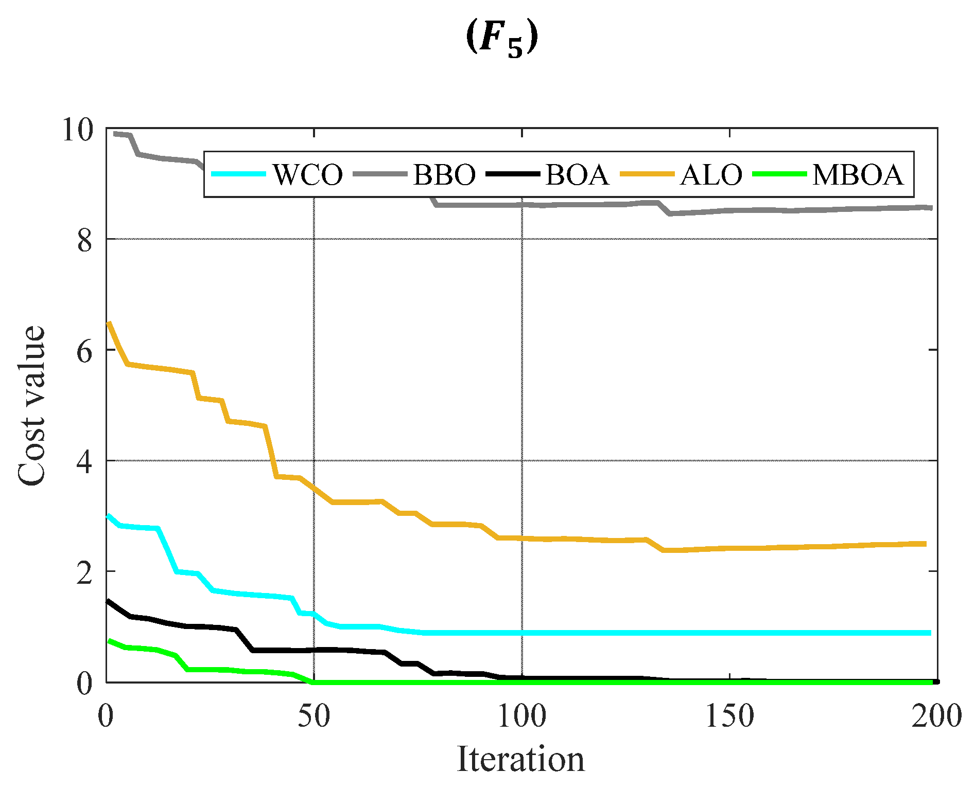
To show further validation of the proposed algorithm, it has been compared with some other state-of-the-art algorithms, as concerns the convergence rate. The convergence diagram of the compared algorithms is depicted in Figure 2.

As can be observed from this figure, it can be stated that the suggested algorithm gives the best convergence rate in comparison with the other comparative algorithms, which shows the better accuracy and consistency of the presented method.

This paper aims to minimize the objective functions, which are the CO₂ equivalent emissions and life-cycle costs (LCC) [30], through a simulation process. LCC means considering all the costs that will be incurred during the lifetime of the building: purchase price and all associated costs (delivery, installation, insurance, etc.).

2.2. Design Variables

Building envelope components, including the roof, glazing type, wall, floor, and ceiling materials, are included in the design variables. Due to the fact that dealing with discrete variables is complicated in numerical optimization approaches, these variables are considered continuous. Nevertheless, it is noteworthy that the optimal values achieved here are unavailable in the market, which leads to conflict between optimization proposals for materials according to numerical achievements and elements generally utilized in designing [31]. To deal with this clear conflict problem, all considered variables are only materials and are discrete. The assumed variables in the process of optimization are accessible in the market. The design variables applied to the case study here with related variation ranges are stated in

Table 4. The design variables with a related variation range [31].

Definition	Exterior Walls: Living Room				Definition	Ceiling: Living
Layer	L 1	Layer	L 3	L 4	Layer	L 1	L 2
Variable	$V_a$	Variable	$V_c$	$V_d$	Variable	$V_o$	$V_p$
Range	12, 13	Range	23, 26–39, 45, 46	8–11	Range	22, 24–33, 40–44	8–11
Definition	Internal walls				Definition	Ceiling: Attic
Layer	L 1		Layer	L 3	Layer	L 1
Variable	$V_e$		Variable	$V_g$	Variable	$V_q$
Range	8–11		Range	8–11	Range	8–11
Definition	Floor: Garage				Definition	Gable
Layer	L 1				Layer	L 1
Variable	$V_h$				Variable	$V_r$
Range	18–21				Range	14–16
Definition	Floor: Living				Definition	Garage: Door
Layer	L 1		L 2		Layer	L 1
Variable	$V_i$		$V_j$		Variable	$V_s$
Range	18–21		47–49		Range	50
Definition	Roof				Definition	Ceiling: Garage
Layer	L 1		L 2		Layer	L 1
Variable	$V_k$		$V_l$		Variable	$V_t$
Range	1–7		14–16		Range	8–11
Definition	Exterior walls: Garage				Definition	Windows
Layer	L 1		Layer		Layer	L 1	L 2
Variable	$V_m$		Variable		Variable	$V_u$	$V_v$
Range	12, 13		Range		Range	52–72	3, 6, 8, 13

.

2.3. Objective Functions

The minimization of the CO₂-eq emissions and the life-cycle costs is the target in this paper. Residential buildings are assumed to be studied herein. Indeed, the considered objectives are conflicting. High-energy-efficiency materials may have less environmental benefit than low-energy-efficiency ones, while the cost of materials that benefits the environment is often more than the same customary materials. Consequently, a multiple-objective optimization (MOO) [32] technique is required. A Pareto frontier is required to help the decision maker to quickly evaluate the balance between the two objectives. A Pareto optimum is a solution to the MOO problem that lowers an objective with no simultaneous effect on the other objective. The Pareto frontier is the plot of the objective function in which its non-dominated vectors are in the Pareto optimum set that is non-dominated. A Pareto frontier [33] whose objectives are LCC and carbon dioxide emissions is depicted in Figure 3 as an example.

Figure 4 shows all the steps of a building’s lifetime in the life-cycle evaluation of residential buildings. These steps are the before-use step, which includes extracting raw materials and processing them, producing components for construction, transporting the materials, and constructing the building; the use step, which consists of all emissions in 25 years of the building‘s life use, concerning the building maintenance in addition to the utilized energy for cooling, heating, lighting, and equipment; and the after-use step, which includes the building demolition and then transferring waste.

The LCC formula of the building is defined as follows [35]:

$$LCC=I{C}_p+S{C}_{cv}+E{C}_{cv}+OM{RC}_{cv}$$

(16)

where $I{C}_i$ is the primary investment cost. $S{C}_{cv}$ denotes the current value of substitution costs. $E{C}_{cv}$ refers to the current value of energy costs. $OM{RC}_{cv}$ is the current value of operating, maintenance, and repair costs.

RSMeans data as the primary data are used to obtain construction cost data [36], including the costs of labor, materials, equipment, and replacement. The LCC evaluation is considered for the life span of 25 years as aforementioned.

The yearly report of the United States Department of Energy (DOE) [37] is used for the energy escalation rates as the secondary data. The minimization of carbon dioxide emissions in the building’s lifespan is the next objective. Carbon dioxide, methane, and nitrous oxide are considered herein as emissions. The Global Warming Potential (GWP) [38] factor for CO₂, CH₄, and N₂O is equal to 1, 21, and 256, respectively. 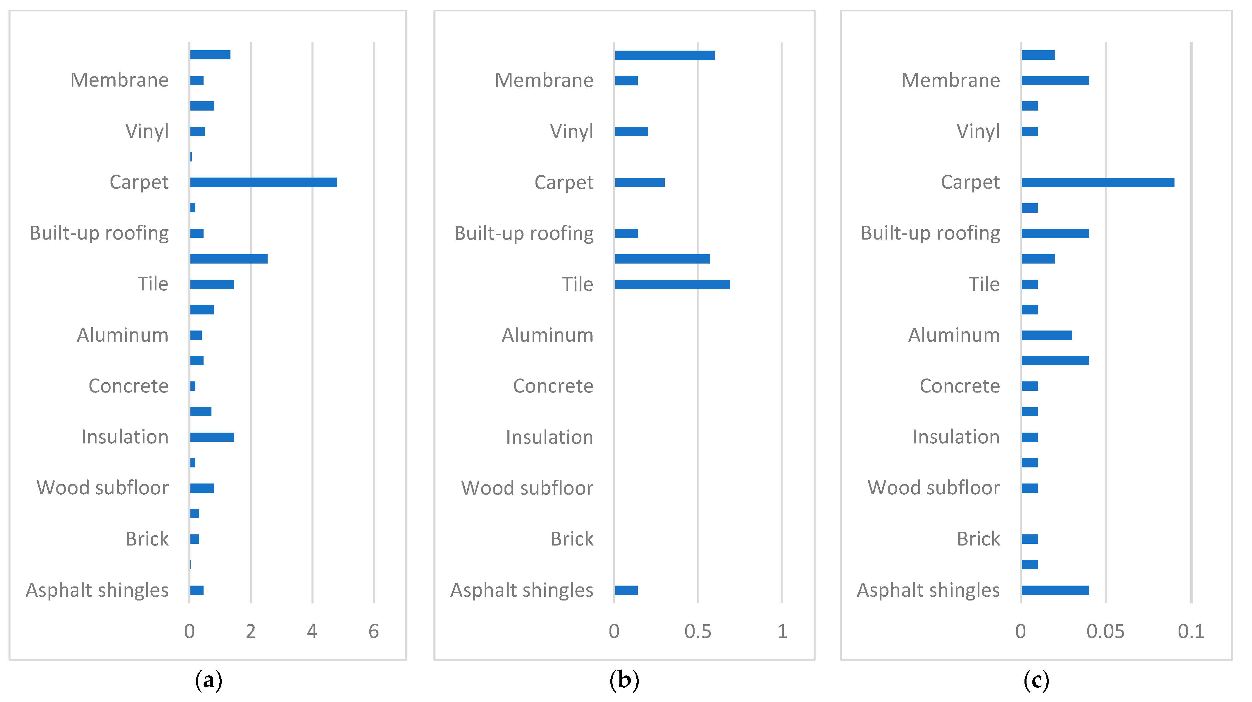Some life-cycle assessment (LCA) [39] datasets have been used for the GWP data of all materials. All materials’ emission data applied herein are illustrated in Figure 5.

According to the GWP data at all steps, the emission lifetime for each design has been computed. First, when calculating before-use step emissions of a building, each mass of material must be calculated. After that, based on the data provided in Figure 5, the associated emissions of the extraction of raw material and the manufacturing of materials is measured.

Two parts are included in the use-step emissions, which are the electrical power use emissions in the building and building maintenance emissions during the life cycle of it. The needed yearly cooling–heating load is first measured for the determination of the electrical power-associated emissions. Second, the factors of the local electrical power emissions have been applied for the determination of the emission factor of the electrical power use. The electrical power emissions factors of the Louisiana average that are defined by the Emissions and Generation Resource Integrated Database (eGRID) [40] have been applied herein. Then, to achieve the first part of the use-step lifetime emissions, the yearly emissions have been multiplied by 25 years. A series of materials, which are required to be replaced within a defined period during the life cycle of a building, have been specified for the next part of the emissions calculation. The GWP [38] of the substituted materials has been measured in a similar way to the main construction materials. In the end, the amount is included in the use-step emissions. Notably, the emissions related to the extracting, processing, and transporting of materials and fuels utilized at the plants are not considered in eGRID. Therefore, the total energy chain is not investigated in this study. All emissions are concerned with the lifecycle of demolition and transportation to recycling or disposal sites. The factors of the emissions related to this step are given in Figure 5 [41,42].

Figure 5. The GWP of Materials [16,41,42]. ((a): before-use, (b): use; (c): after-use emissions by mass (kg CO₂-eq)).

Figure 5. The GWP of Materials [16,41,42]. ((a): before-use, (b): use; (c): after-use emissions by mass (kg CO₂-eq)).

In the current study, first, the geometry of the building, meteorological information, occupation scheduling, lighting, and HVAC system [43] are defined. Then, the primary amounts of design variables are determined randomly by the Improved Billiard-based Optimization Algorithm. The design variables are the materials of the building envelope.

After that, for the evaluation of the life cycle cost and emissions of the defined model, a simulation is performed. For cooling, heating, ventilation, and lighting modeling, EnergyPlus [44] is used, which is a dynamic energy simulation tool for modeling the energy consumption of the whole building. Natural ventilation systems, multiple-zone airflow, and thermal comfort can be modeled in this software. Then, the values of the design variables are updated by the IBOA algorithm according to the achieved results, and for the evaluation of the life cycle cost and emissions of the updated design, another simulation is carried out. The highest number of iterations for the IBOA algorithm is considered to be equal to 150. We continued the process of simulation until reaching this amount.

In this study, to estimate foundation CO₂ emissions, the following steps have been conducted:

-

Identifying emission sources: identifying the activities related to the foundation that contributes to CO₂ emissions.

-

Gathering data: the data on the energy consumption of foundation, transportation, and waste generation have been collected.

-

Determining emission factors: emission factors are conversion factors that relate the quantity of a specific activity to the amount of CO₂ emitted. The reliable source for emission factors was the U.S. Environmental Protection Agency (EPA) [45].

-

Calculating emissions: the data collected in step 2 are multiplied by the appropriate emission factors from step 3 to calculate emissions for each activity.

-

Aggregating emissions: the emissions from all activities are summed up to obtain the total CO₂ emissions of the foundation to estimate the foundation’s carbon footprint.

2.4. Case Study

A single-family house located in Atlanta, a city in Georgia, USA, was selected to be studied in this study. The climate of Georgia is humid and subtropical, with most of the state having short, mild winters and long, hot summers. The average temperatures for the mountain region in January and July are 39 °F (4 °C) and 78 °F (26 °C), respectively. Winter in Georgia is characterized by mild temperatures and little snowfall around the state, with the potential for snow and ice increasing in the northern parts of the state. Summer daytime temperatures in Georgia often exceed 95 °F (35 °C). Figure 6 shows the design of this house.

The area of the house is equal to 190 m². The space of the house is divided into three zones: case (I): living space (conditioned), case (II): garage (unconditioned), and case: (III) attic (unconditioned). The ASHRAE standard [46] is used for the estimation of internal heat gains generated by the activity of occupants as metabolic heat, by utilization of electrical devices, or by thermal emission of artificial lighting [47]. These values are calculated monthly. For space heating and cooling, an air source heat pump ventilation system has been utilized. The cooling and heating indoor temperatures are designed to be equal to 26 °C and 22 °C, respectively.

Demographic statistics for Atlanta, including variables such as age, gender, place of residence, and level of education are reported in

Table 5. The demographic statistics table.

Variable	Category 1	Category 2	Category 3	Category 4	Category 5
Age group	0–17 years	18–24 years	25–34 years	35–44 years	45+ years
Gender	Male	Female	Non-binary/Other	-	-
Place of Residence	Downtown	Midtown	Buckhead	Westside	East Atlanta
Level of Education	High School or Less	Some College	Bachelor’s Degree	Master’s Degree	Doctorate or Higher

.

This table provides a breakdown of the population in Atlanta based on different demographic variables. The categories for each variable are listed in the table, allowing us to organize and analyze the data effectively.

The major differences that contribute to variations in CO₂ emissions in Atlanta can be attributed to several factors including: (a) Energy sources: the primary source of electricity generation can significantly impact CO₂ emissions. Buildings that rely heavily on fossil fuel-based power plants, such as coal or natural gas, tend to have higher emissions compared with those with a greater share of renewable energy sources like solar, wind, or hydroelectric power. (b) Industrial activities: energy-intensive buildings have higher CO₂ emissions. (c) Transportation: the transportation sector is a major contributor to CO₂ emissions. (d) Building efficiency: the energy efficiency of residential buildings plays a significant role in CO₂ emissions. Buildings with older infrastructure, inadequate insulation, and inefficient heating, ventilation, and air conditioning (HVAC) systems have higher emissions compared with buildings with newer and more energy-efficient structures. (e) Waste management: the handling and treatment of waste also contributes to CO₂ emissions. Buildings with inefficient waste management practices may experience higher emissions compared with buildings that prioritize recycling, composting, and energy recovery from waste. (f) Urban planning and land use: the layout and design of a city affect transportation patterns and energy consumption. Cities with well-planned public transportation systems, mixed land-use zoning that reduces the need for long commutes, and infrastructure that promotes active modes of transportation like walking and cycling tend to have lower CO₂ emissions. (g) Climate and weather patterns: climate conditions affect energy demand for heating or cooling, as well as the prevalence of certain industries. For example, cities in Georgia with warmer climates have higher energy demands for air conditioning, while cities with colder climates have higher heating-related emissions.

These factors, among others, contribute to variations in CO₂ emissions between buildings in Atlanta. It is important to note that the specific characteristics and policies of each building can further influence emissions, making it necessary to assess the unique circumstances of a particular building when estimating and comparing CO₂ emissions. The factors mentioned refer to CO₂ emissions during the operational stage. These factors are commonly associated with the direct emissions resulting from activities within the city, such as energy consumption, industrial processes, and transportation activities. However, when assessing CO₂ emissions comprehensively, it is important to consider emissions across different stages of the life cycle of the building. This approach is known as a life-cycle assessment (LCA).

A life-cycle assessment takes into account the emissions related to various stages, including: (a) Extraction and production of raw materials: this stage involves the extraction and processing of materials used for infrastructure and buildings. Emissions can result from mining, manufacturing, and transportation of these materials. (b) Construction and infrastructure development: the construction stage includes emissions related to the fabrication, transportation, and assembly of materials, as well as the energy consumption during the construction process. (c) Operation and maintenance: as mentioned earlier, this stage focuses on the emissions resulting from day-to-day activities, such as energy consumption, transportation, and waste management. (d) End of life and disposal: this stage involves the decommissioning, demolition, and disposal of infrastructure and buildings. Emissions can arise from activities such as waste disposal, energy-intensive demolition processes, and the release of stored carbon from materials. By considering the entire life cycle of a building, including both direct and indirect emissions related to different stages, a more comprehensive understanding of its carbon footprint can be obtained. This approach helps to identify opportunities for emission reductions at various stages and informs sustainable planning and decision-making processes.

3. Results and Discussions

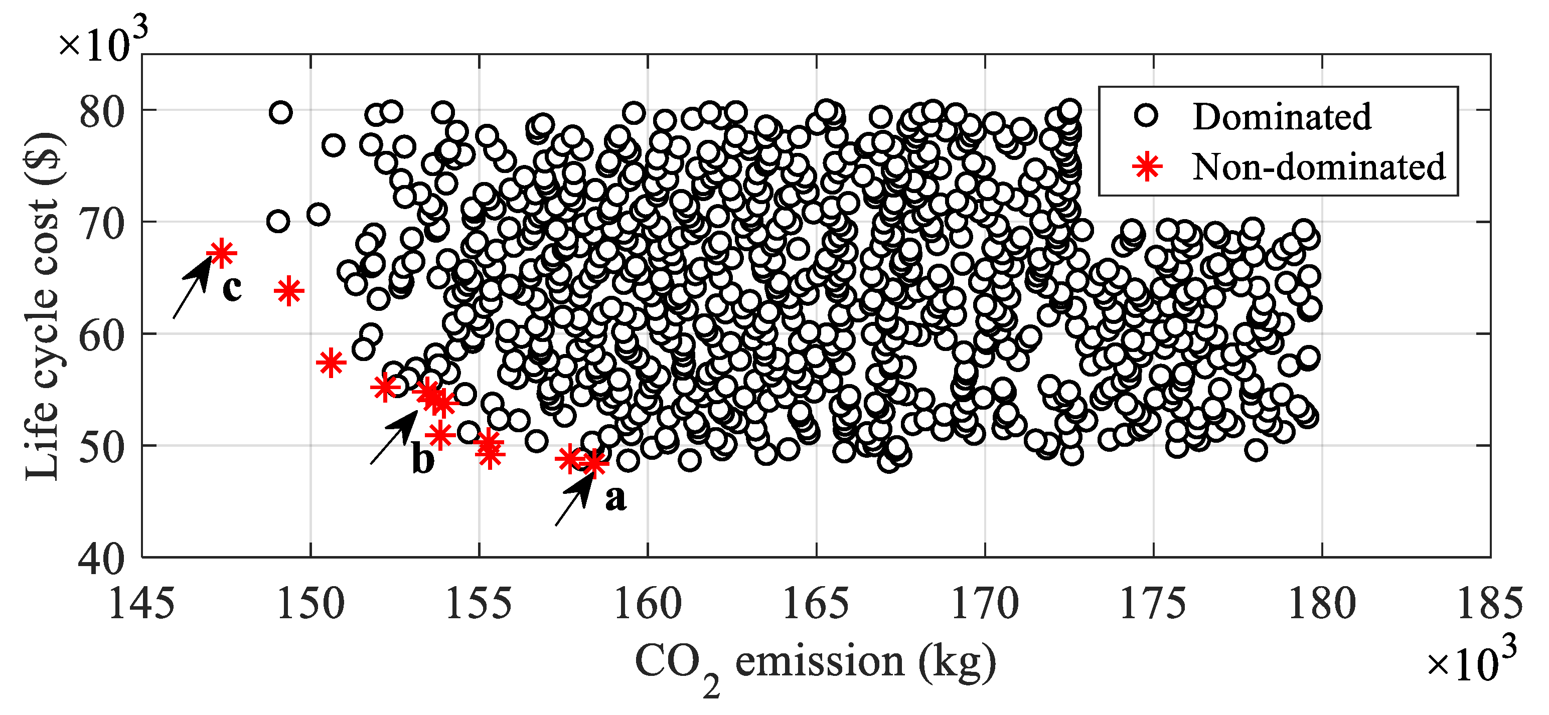
The results of the optimization method are provided in this section. It took 90 s for each simulation on average on the defined system. The Pareto frontier solution of carbon dioxide emissions and life-cycle costs is depicted in Figure 7.

A decrease in carbon dioxide emission is obtained by an increase in the LCC, as seen in this figure. Figure 7 shows the optimum favored solutions for all criteria at lower or higher levels. As can be observed, point “a” with low cost has a high environment-related effect, solution “b” gives medium amounts for both LCC and CO₂ emission, and solution “c” with high cost gives a low environment-related effect. When only the minimization of life-cycle costs is aimed for independently without considering the carbon dioxide emissions reduction, point “a” can be the optimum solution. But, when the optimization of carbon dioxide emission is performed independently, point “c” is the proper point. It should be noticed that the rate of life-cycle costs for carbon dioxide emissions is equal to −0.188 in point “c”, considering that this amount is equal to −3.548 in point “a”. This indicates that the potentiality of point “c” is lower than “a” in reducing carbon dioxide emissions. This can be the reason that a small increase in life cycle costs can cause a significant decrease in carbon dioxide emissions.

As mentioned, the three optimum Pareto solutions are a, b, and c. V_a–V_v are the defined 22 variables. For all three solutions, V_a is the Vinyl. For V_b, Plywood with 13 mm, 13 mm, and 10 mm thickness is considered for Pareto optimum solutions a, b, and c, respectively. V_c is blanket fiberglass-6″ for solution a and cellular for both solutions b and c. For V_d, gypsum with 16, 16, and 9.5 mm are used for Pareto optimum solutions a, b, and c, respectively. Also, V_e is gypsum with 16, 13, and 16 mm. V_f is blanket insulation-6″, Rigid fiberglass-3.5″, and Cellular polyurethane-2″ for solutions a, b, and c, respectively. For V_g, gypsum 9.5 mm, wood ceiling, and gypsum 13 mm are used for solutions a, b, and c, respectively. V_h is concrete 150, 50, and 100 mm for Pareto optimum solutions a, b, and c, respectively. Also, for V_i, concrete with 100, 50, and 50 mm are considered. V_j is defined as carpet, carpet, and wood subfloor, respectively, for solutions a, b, and c, respectively. The membrane is used for all solutions for V_k. The applied materials for V_l are plywood with 10, 13, and 16 mm. V_m is vinyl for solutions a and c, and wood for solution b. Variable V_n is defined as plywood with thicknesses of 10, 16, and 10 mm, respectively, for solutions a, b, and c. Fiberglass insulation-8.8″ and 13″ are used for solutions a, and b, for variable V_o, and c is mineral wool insulation-13″. The materials for V_p are gypsum with thicknesses of 16, 9.5, and 13 mm. Also, V_q is gypsum with thicknesses of 13, 9.5, and 9.5 mm. All solutions are plywood 10 mm for V_r. V_s is a steel door, which is the same for all three solutions. For V_t, gypsum with 13, 16, and 13 mm thicknesses, respectively, for a, b, and c is considered. For V_u, Ref A Clear Lo 6 mm is used for all solutions. V_v is the air gap of 8, 13, and 13 mm. These materials are utilized in the envelope of the house in all cases. Emissions equal 157,917, 152,781, and 146,803 kg for solutions a, b, and c, respectively. The value of the life-cycle costs are 48,329$, 54,058$, and 67,180$, respectively, for solutions a, b, and c.

The overall GWPs for all cases, including (I), (II), and (III), are stated in

Table 6. Life cycle global warming potential.

CO2 Emission (kg) Thousands	Case (I)	Case (II)	Case (III)
Before-use	20,360	17,050	16,553
Use	137,118	130,122	131,213
After-use	189	71	128

, which contains all the global warming potential gases released into the surroundings while extracting the raw materials and processing them; manufacturing and transporting them; constructing the building in the before-use step; the maintenance in the use step; and the life-cycle demolition and transportation to recycle or disposal sites in the after-use step.

A comparison among all cases shows that the overall GWP for case (I), the maximum one, is equal to 157,667 kg of CO₂-eq. The carbon dioxide emission of the before-use step is equal to 20,360 kg, which is 12.9% of the overall life cycle. This amount for the use step is equal to 137,118 kg (almost 87% of the life cycle), and for the after-use step, it is equal to 189 kg, which is about 0.12% and insignificant. But, the minimum emission belongs to case (III) among three cases. The value of the carbon dioxide emission for case (III) is equal to 17,050 kg in the before-use step, which is 11.6% of the overall life cycle. In comparison with case (I), this amount is 23% lower. The emission of the use step is equal to 130,122 kg, which is almost 88.4% of the overall life cycle (4.5% lower than case (I)).

As shown in

Table 7. The carbon dioxide emissions for various constructions.

CO2 Emission (kg)	Case (I)	Case (II)	Case (III)
Foundation	10,685.07	4828.50	5739.44
Roof	1063.21	1338.49	1701.80
Ceiling	2729.53	3916.61	3972.00
Walls	1658.25	1978.20	1539.41
Floor	3518.69	3519.56	2243.38
Windows	1577.06	1659.29	1618.67
Others	827.52	785.06	788.05

, three scenarios for various construction changes have different life spans for their global warming potential. These variations are related to the foundation, windows, ceiling, walls, roof, and floor. The global warming potential of the use step has not been considered in Table 7.

It can be observed from this table that the maximum life span global warming potential refers to the foundation, due to the materials utilized when constructing it. However, it should be considered that the emissions value of the foundation is different for all cases. The emissions value of the foundation for case (I) is 55% more than case (II). Indeed, the minimum emissions value of the foundation belongs to case (II). In case (I), the higher thickness of concrete utilized when constructing the foundation is the reason for the higher value of emissions. The highest values of emissions refer to the ceiling and floor, respectively, after the foundation, which is because of the high emissions of the utilized materials in their construction.

Policy Recommendations

The offered optimization method can find the most efficient strategies for a given case building. The findings from this method have been intended to inform policy makers about optimum optimization solutions for different building zones. This information can be utilized as the foundation for developing an optimization technique for a given building. To allow the decision maker to quickly evaluate the trade-off between the two objectives, a Pareto front has been plotted herein. According to the preference of the decision makers, different solutions can be selected among the Pareto optimum solutions a, b, and c. Figure 7 depicts the optimum desired solutions for all criteria at lower or higher levels. A decrease in carbon dioxide emissions is obtained through an increase in the LCC, as seen in this figure. As can be observed, point “a” with a low cost has a high environment-related effect, solution “b” gives medium amounts for both LCC and CO₂ emissions, and solution “c” with a high cost gives a low environment-related effect. When only the minimization of life-cycle costs is aimed for independently, without considering the carbon dioxide emissions reduction, point “a” can be the optimum solution. But, when the optimization of carbon dioxide emissions is performed independently, point “c” is the proper point.

The data summary is stated in

Table 8. Data summary table.

CO2 Emission (kg)	Min	Average	Max
Foundation	4828.50	7084.34	10,685.07
Roof	1063.21	1367.83	1701.80
Ceiling	2729.53	3539.38	3972.00
Walls	1539.41	1725.29	1978.20
Floor	2243.38	3093.88	3519.56
Windows	1577.06	1618.34	1659.29
Others	785.06	800.21	827.52

.

Furthermore, a comparison of the achieved LCC and the emission results using the proposed method (Improved Billiard-based Optimization Algorithm (IBOA)), with some other state-of-the-art methods from the literature including Non-dominated sorting genetic algorithm II (NSGA-II) [18], Grey Wolf Optimizer GWO [36], and genetic algorithm (GA) [23], has been carried out and the results are reported in

Table 9. The results of the comparison of the proposed method with some other state-of-the-art methods.

Methods	IBOA	NSGA-II [19]	GWO [48]	GA [23]
LCC ($)	56,522	61,749	59,887	68,345
Emissions (kg)	152,500	159,442	156,211	161,569

.

Based on Table 9, a comparison of the results of the proposed method with some other state-of-the-art methods from the literature showed that the proposed method gives better results and a minimum value of the LCC and emissions compared with the others.

4. Conclusions

To design buildings with lower emissions and higher energy efficiency, we aimed to minimize the carbon dioxide equivalent emissions and life-cycle costs (LCC) of buildings in this paper. A multiple-objective optimization method based on a new metaheuristic algorithm, called the Improved Billiard-based Optimization Algorithm (IBOA) has been presented. There are different methods to solve the optimization problems. Based on the NLP theory, there is not any metaheuristic algorithm that can solve all the problems accurately. Sometimes, the answer to the basic algorithm is the local optimum. Therefore, to reach the global optimum, we proposed this algorithm. Moreover, in some cases, the basic model suffers from premature convergence, which avoids reaching an accurate result. In this paper, a solution to this problem has been proposed to obtain better convergence results using the proposed method. The competitive objectives included a decrease in financial costs, a reduction in environment-related effects, and the optimization of energy consumption. For the building simulation, the EnergyPlus software was selected. A single-family house was chosen to test the proposed model, which was in Atlanta, a city in Georgia, USA. To obtain a balance between the environmental and economic performance of the building, the set of Pareto optimum solutions that were achieved can be effective for designers. The suggested optimization method identified the most efficient strategies for a given case building. The findings from this method have been intended to inform policy makers about optimum optimization solutions for different building zones. This information can be utilized as the foundation for developing an optimization technique for a given building. A comparison of the results of the proposed method with some other state-of-the-art methods from the literature showed that the proposed method gives better results and minimum values for the LCC and emissions. For future works, the design of the optimal envelope of the building for various weather conditions will be attempted. Furthermore, the impact of various HVAC systems to achieve optimal designs can be considered. Some variables are effective and commonly used in design practice, but these are not available in the market (the limitation of this study), which can be considered in the future direction of research.