Article

Post-Earthquake Damage Identification of Buildings with LMSST

1
Department of Electronic and Information Technology, Miami College, Henan University, Kaifeng 475004, China
2
Department of Instrumentation and Control Engineering, Manipal Institute of Technology, Manipal Academy of Higher Education, Manipal 576104, India
3
Department of Civil Engineering, Miami College, Henan University, Kaifeng 475004, China
*
Authors to whom correspondence should be addressed.
Buildings 2023, 13(7), 1614; https://doi.org/10.3390/buildings13071614
Submission received: 13 April 2023 / Revised: 25 May 2023 / Accepted: 30 May 2023 / Published: 26 June 2023

Abstract

:
The structure is said to be damaged if there is a permanent shift in the post-event natural frequency of a structure as compared with the pre-event frequency. To assess the damage to the structure, a time-frequency approach that can capture the pre-event and post-event frequency of the structure is required. In this study, to determine these frequencies, a local maximum synchrosqueezing transform (LMSST) method is employed. Through the simulation results, we have shown that the traditional methods such as the Wigner distribution, Wigner–Ville distributions, pseudo-Wigner–Ville distributions, smoothed pseudo-Wigner–Ville distribution, and synchrosqueezing transforms are not capable of capturing the pre-event and post-event frequency of the structure. The amplitude of the signal captured by sensors during those events is very small compared with the signal captured during the seismic event. Thus, traditional methods cannot capture the frequency of pre-event and post-event, whereas LMSST employed in this work can easily identify these frequencies. This attribute of LMSST makes it a very attractive method for post-earthquake damage detection. In this study, these claims are qualitatively and quantitatively substantiated by comprehensive numerical analysis.

1. Introduction

In recent decades, the number of multi-story buildings has exponentially increased due to the urbanization and availability of modern technology and construction materials. Post-earthquake damage assessment of buildings is necessary for seismic risk mitigation and resilience planning [1]. With recent progress in signal processing and sensor technology, damage detection using data collected from the sensors attached to buildings is becoming very popular in structural health monitoring (SHM) [2,3]. Modal parameters such as damping ratio, mode shape, and natural frequency are the key parameters to assess the dynamic characteristics of a building. When a structural system changes mass, stiffness, or structural damping, the values of the parameters tend to vary. This approach can identify the damaged state of the structure [4]. Recently, many researchers have employed time history analysis and Fourier transform (FT) for damage detection. The shifting of a structure’s frequency components during an earthquake may be caused by nonlinearities such as the surrounding environment, degree of excitement, and earthquake ground motion. If the frequency fluctuation ceases after the earthquake and returns to the pre-event frequency of the building (i.e., the natural frequency of the building), there is no structural damage. However, if there is permanent structural damage, then the natural frequency of the building permanently changes [5]. Damage identification and real-time health monitoring can be performed by comparing the pre-event and post-event frequencies of the building [6]. For this purpose, a joint time-frequency (TF) method is required as this method simultaneously provides the time and frequency information of a signal. Black [7] applied a short-time Fourier transform (STFT) on the data collected from the Sheraton Universal Hotel located in Los Angeles, USA, to identify the damage. The study demonstrated that the natural frequency of the building remained stationary even after the earthquake, and hence, it was concluded that there was no damage to the building. The damage to the building has also been identified using Wigner–Ville distribution (WVD). The presence of cross-terms in WVD hinders the interpretations and creates a significant barrier to understanding the response of the building. To overcome this drawback, extended versions of the WVD, such as pseudo-Wigner–Ville distribution (PWVD), smoothed pseudo-Wigner–Ville distribution (SPWVD), and reassigned smoothed pseudo-Wigner–Ville distribution (RSPWVD), were employed for damage detections and other signal processing applications [8,9,10,11]. Similarly, various TF methods, such as STFT, S-transform (ST), and local time-frequency transform (LTFT), were also employed for damage detection [12]. It was reported that the TF method with less cross-term interference and the least Renyi entropy is suitable for damage detection. Similarly, the performances of the Gabor–Wigner transform (GWT), S-transform, synchrosqueezing transform (SST), and other time-frequency methods were compared in [13]. It was concluded that the SST is the best among all methods. However, SST suffers from a smearing problem and is not capable of capturing the pre-event and post-event frequencies of the structure.
During the seismic event, the amplitudes of the signals captured by the sensors are relatively high due to external excitations (i.e., an earthquake). The inertia of the building may prevent a sudden decline in the magnitude of the post-event signal following an earthquake. A certain amount of time must pass before the structure settles and reaches a stable state. In post-earthquake damage detection, the primary goal is to analyze the building’s fundamental frequency during this stable state, both before and after seismic events. In both cases, the amplitudes of the signals captured by the sensors are relatively low; with traditional TF methods, it is challenging to deal with low-amplitude signals [14]. In this regard, the local maximum synchrosqueezing transform (LMSST) stands out as a highly sensitive method for detecting amplitude-weak modes [14], making it a suitable choice for post-earthquake damage detections.
In this research, LMSST is employed for damage detection. The usefulness of LMSST is demonstrated using multi-component synthetic signals and various real earthquake data. Through visual representations and qualitative measures, it is observed that LMSST has a better TF resolution and can detect post and pre-event frequencies of the structure, which play a very critical role in structural health monitoring. The amount of permanent shift at the natural frequency of the building after any seismic event determines the health of the building [3,6,11]. This research work is organized in the following manner: in Section 2, various TF methods are discussed, followed by a discussion on Rényi entropy and the analysis of the results in Section 3 and Section 4, respectively. The paper is concluded in Section 5.

2. Time-Frequency Methods

2.1. Wigner Distribution

The Fourier transform of the autocorrelation of the input signals is defined as the Wigner distribution. WD is mathematically expressed by the following equation:
W D s ( t , f ) = + s t + τ 2 + s t τ 2 e j 2 π f τ d τ
where ∗ is the complex conjugate of a real signal. WD enhances time and frequency resolutions. However, low-frequency artifacts due to the interactions of positive and negative frequencies in the time-frequency plane were studied [8,15,16]. By modifying the WD with the analytic signal, these artifacts can be reduced, and it is now called Wigner–Ville Distribution (WVD). Mathematically, WVD could be expressed by
W V D b ( t , f ) = + b t + τ 2 b t τ 2 e j 2 π f τ d τ
where b t is the Hilbert transform of the input signal. The analytic signal’s Fourier transform is given by
b ( f ) = { 2 S ( f ) , i f f > 0 S ( f ) , i f f = 0 0 , i f f < 0
where b f is an analytic signal of   s t . Thus, it can be assumed that the WVD is an extension of WD. The analytic signal removes the low-frequency artifacts; however, the cross-term interference caused by the actual frequency components cannot be eliminated, which exhibits the disturbing tendency in the time-frequency plane and provides misleading information [15,17]. Despite these drawbacks, it has been shown that the WVD concentrates the signal energy along with the instantaneous frequency. As a result, the WVD serves as the foundation for separating seismic events in the time–frequency plane.

2.2. Smoothed Wigner–Ville Distribution

The Pseudo Wigner–Ville Distribution (PWVD) is expressed by the following equation:
P W V D z ( t , f ) = + d ( τ ) z ( t + τ 2 ) + z ( t τ 2 ) e j 2 π f τ d τ
WVD provides time–frequency resolution to a large extent. However, one of the major challenges in WVD is the cross-term interference, which can be suppressed in the time–frequency plane with a sliding window, d τ . PWVD improves the resolution, although it has interference terms that can make elucidation difficult [18]. Because of this problem, PWVD has now been modified and is now known as SPWVD that can be expressed mathematically as follows:
P ( t , f ; m , n ) = + n ( τ ) + m ( u τ ) e j 2 π f τ x a ( u + τ 2 ) x a ( u τ 2 ) d u d τ
SPWVD is a windowed version of WVD that achieves a better time–frequency resolution by using independent time and frequency window functions. Window functions m and n suppress cross-term interference along the time axis and the frequency axis, respectively. SPWVD is also used in pulse oximetry to reduce motion artifacts, which enhances the accuracy of wearable devices [19]. In addition to this, decompositions of the seismic spectra of a sandstone dam were performed using the SPWVD in the West Sichuan depression to detect the hydrocarbon. The degree of smoothing depends on the width of the window function

2.3. Synchrosqueezing Transform

Synchrosqueezing transform is a widely used joint time–frequency method that reassigns the signal’s energy along the frequency axis while preserving the signal’s time resolution. Secondly, this method controls the leakage/spreading effect caused by the mother wavelet, and in turn, enhances the time–frequency resolution to some extent [20]. The SST is a consistent and powerful mathematical tool that is used to detect frequency components, which have been further used in various applications [21,22]. The wavelet transform mathematical equation is defined as
W m , τ = s t 1 m ψ t τ m d t
where s(t) is the time domain signal, ψ t is the mother wavelet, τ indicates translation of the window function, and m is the scale of the mother wavelet, which is responsible for dilating and compressing the window. After computing the wavelet coefficient   W m , τ from the input signal, the instantaneous frequency is to be extracted at any point   m , τ .
ω ( m , τ ) = j W ( m , τ ) W ( m , τ ) τ
The wavelet coefficient is calculated only on a discrete scale (   m k ). The SST T s ω , τ can be computed at the centers of the frequency ω l with ω l ω l 1 = Δ ω .
T s ( ω l , τ ) = 1 Δ ω a k : ω ( a k , τ ) ω k Δ ω / 2 W ( m k , τ ) m k 3 / 2 Δ m k
SST improves the time–frequency resolution to some extent. However, the variations of frequency components are difficult to distinguish due to the blurring effect.

2.4. Local Maximum Synchrosqueezing Transform

The analysis initiates with the fundamental concept of STFT, which has become the most powerful mathematical tool for analysis of seismic signals. The STFT is expressed by Equation (9).
S T F T t , w = s t w t τ e j ω τ d
where w t is a window function and τ indicates the position of the window. STFT divides the signal into small segments called windowed signals, i.e., s t w t τ , and the width of the window function determines its resolution [15,23,24]. Taking the square of the magnitude of the STFT yields the spectrogram shown below.
S P S T F T t , f = S T F T t , f 2 = s t w t τ e j ω τ d τ 2
It is possible to model a multi-component signal with the frequency-modulated (FM) and amplitude-modulated (AM) laws as
s t = k = 1 n a k t e i ϕ k t
where   a k t is the instantaneous amplitude (IA) and ϕ k ' t is an instantaneous frequency (IF). The IA and IF are two significant features that are used to gain insight into the signals’ time-varying characteristics. However, STFT has poor time and frequency resolutions and provides smeared energy distribution. To obtain sharper results, SST was recently introduced, which reassigns the existing time–frequency coefficients into the newly measured time–frequency position. However, the SST method also provides a poor energy concentration in the time–frequency plane. Recently, a local maximum synchrosqueezing transform (LMSST) was proposed, which increases the time–frequency resolution of a signal to a large extent [14]. The mathematical expression for LMSST is as follows:
L M S S T t , η = + S T F T t , ω η ω m t , ω d ω
Further, ω m t , ω is a frequency-reassignment operator and can be defined as
  ω m t , ω = a r g m a x S T F T t , ω , ω ω Δ , ω + Δ , i f S T F T t , ω 0 0 , i f S T F T t , ω = 0  
to separate the two arbitrary modes, with the frequency distance ϕ k + 1 t ϕ k t > 4 Δ k 1 , 2 n 1 . The picking of a smoothing filter is an important task. Furthermore, it is supposed that a window function’s Fourier transform reaches its maximum at zero. The operator for frequency reassignment can be written as
ω m t , ω = ϕ k t , i f ω ϕ k t Δ , ϕ k t + Δ 0 ,   o t h e r w i s e
where ϕ k t is the instantaneous frequency. LMSST diminishes the blurring effect and offers a promising approach that can further be utilized in the area of earthquake engineering to detect damage to buildings.

3. Assessment Criteria of Time–Frequency Method

In most cases, it has been observed that visual inspection does not provide a consistent result. Therefore, an objective evaluation method has been developed to identify the best time–frequency method. In this work, Renyi entropy is designated to identify the appropriate time–frequency method.
Shannon first proposed the concept of entropy measurement in 1949. Later, in signal processing, entropy measures were used to quantify information. Renyi entropy is mathematically defined as
R α = 1 1 α l o g 2 + + ρ α n o r m t , f d t d f
Here, α = 3 is selected for analysis [25,26]. ρ α n o r m is the normalized time–frequency distribution, which can be expressed as
ρ n o r m t , f = ρ t , f + + ρ t , f d t d f
The time–frequency methods are quantified using Renyi entropy. The selection of time–frequency methods through visual inspection becomes hard when there are slight changes in two different time–frequency plots. As a result, researchers used Renyi entropy to classify the best time–frequency method and concluded that the lowest Renyi entropy provides the most concentrated time–frequency method [26,27]. Hence, Renyi entropy is employed to inspect the suitable time–frequency method, which can further be applied in the damage detection of buildings.

4. Results and Discussion

To demonstrate the superiority of the LMSST method over WD, WVD, PWVD, SPWVD, and SST methods, a multi-component synthetic signal and the real earthquake data recorded during the San Fernando Earthquake in 1971 and the Northridge Earthquake in 1994 are used.

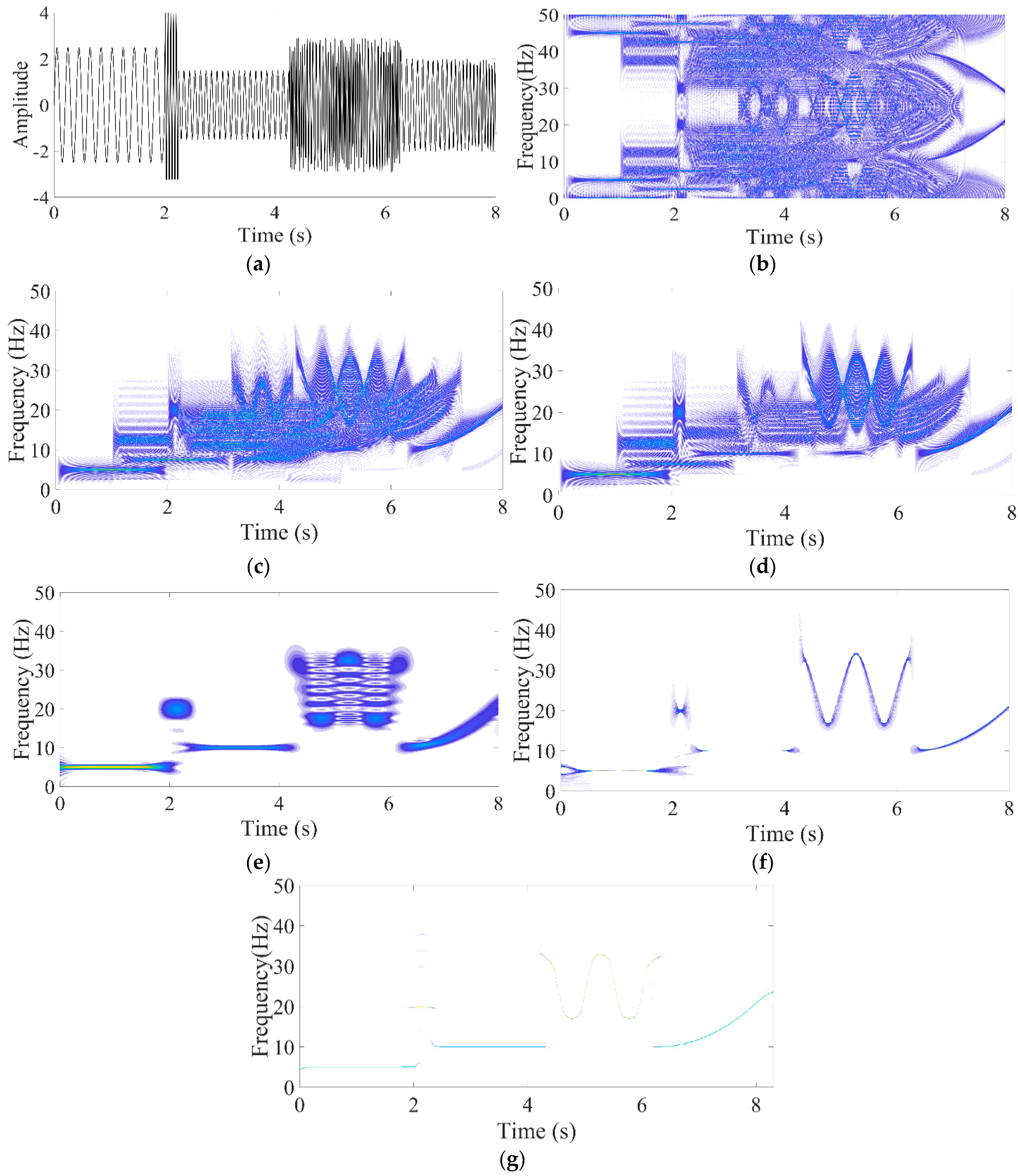
4.1. Synthetic Signal

A synthetic signal comprises of a constant frequency signal, exponentially decaying signal, nonlinear frequency varying signal, and chirp signal is generated using the following equation:
x 1 = 2.5 sin 2 π 5 t ; 0 t 2 x 2 = e t 2 / 10 cos 2 π 20 t ; 2 < t 2.23 x 3 = 1.5   sin 2 π 10 t ; 2.24 < t 4 x 4 = 3 sin 3 150 π t + 3 s i n 2 π t ; 4 < t 6 x 5 = 2 chirp   10   Hz 25   Hz ;   6   <   t     8 y t = i = 1 5 x i
The multi-component signal contains five components with epochs of 2 s, 0.23 s, 1.76 s, and 2 s for the rest of the components, respectively. The time domain representation of a signal is plotted in Figure 1a with a sampling frequency of 100 Hz. The synthetic signal is processed with the help of the WD, WVD, PWVD, SPWVD, SST, and LMSST methods, and the results are plotted in Figure 1b–g, respectively.
From Figure 1b, it can be observed that there are many cross-terms present in the TF plot, and therefore it is almost impossible to extract any meaningful information from it. WD uses the real signal, and hence the positive and negative frequencies generate those cross-term products. In WVD, the cross-terms are minimized by using an analytical signal instead of a real one [23,28]. The analytic signal does not contain negative frequencies and reduces the cross-terms. From Figure 1c, it can be observed that there are still significant cross-terms present between each pair of harmonics that obstruct the proper interpretation of the given synthetic signal.
In PWVD, frequency domain filtering is applied to the signals obtained from WVD, which enhances the frequency domain resolution of the signals, but the resolution in the time domain is still very poor, which can be observed in Figure 1d. In SPWVD, signals obtained from WVD have been filtered in the time domain as well as the frequency domain with the help of the window function. The consequence of using the windowing function is that SPWVD fails to precisely localize the time and frequency components of the signals [9,10]. From Figure 1e, it can be observed that the energy band of each frequency component is very thick and hinders the detection of neighboring frequency components. The result of the SST method is shown in Figure 1g, from which it can be observed that it suffers from the blurring effects in the frequency plane. The result of LMSST is presented in Figure 1g. From the TF plot, it can be observed that LMSST has the sharpest TF plane among all mentioned methods. It achieves such superior TF resolution by detecting the local maxima of the spectrogram in the frequency direction [14].
The Renyi entropy measures of test signal-1 for various TF methods are calculated and presented in Table 1. From the table, it can be observed that among all the employed methods, LMSST has the lowest Renyi entropy. Thus, it can be concluded that it has the most concentrated TF plane among all TF methods discussed so far. Due to the concentrated TF plane provided by LMSST, all the frequency components present in the synthetic signals with their respective occurrences in time epoch can be easily identified in Figure 1g.

4.2. Earthquake Data

The presence of damage in the structures permanently alters their natural frequencies. By examining the pre-earthquake and post-earthquake frequencies of the structures, their respective health can be determined. With appropriate TF tools, this assessment can be quickly and reliably conducted.

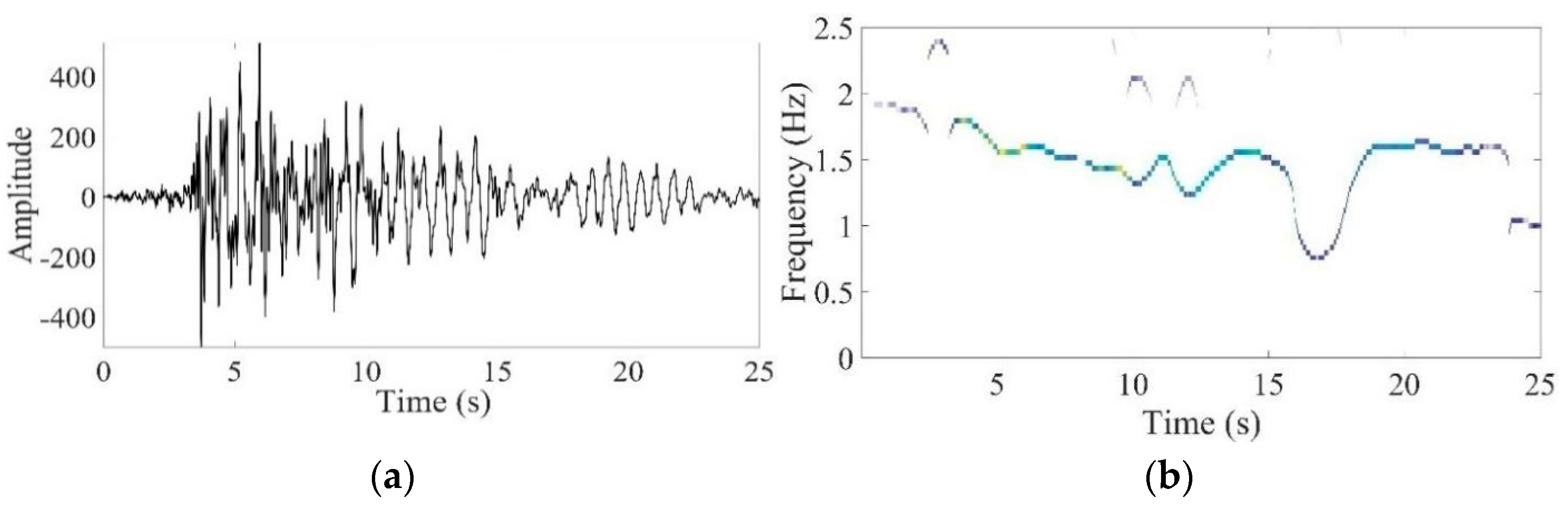
4.2.1. Seismic Data-1: San Fernando Earthquake, 1971

The Millikan Library is a popular and historical nine-story instrumented building constructed in 1966. The San Fernando earthquake occurred in 1971 with a magnitude of 6.6, as mentioned in Table 2. Before the event, two 3-axis Teledyne Geotech RFT-250 accelerometers were placed in the basement and on the roof of the buildings. Figure 2a depicts the time domain responses of the data recorded from the sensor placed on the top floor of the building. The data recorded by the sensor can be classified into three parts: pre-seismic, co-seismic, and post-seismic data [11].
The signals from 0 to 5 s are pre-seismic, 5 to 32 s are co-seismic, and the rest are post-seismic signals. TF representations of earthquake signals for various TF methods, such as WD, WVD, PWVD, SPWVD, and SST, are illustrated in Figure 2b–f, respectively. From the figures, it can be observed that the WD, WVD, PWVD, SPWVD, and SST methods are not capable of capturing the pre-seismic frequencies as well as the tail ends of the post-seismic frequencies. A similar conclusion can be found in [3,11], whereas LMSST has a very well-defined TF plane, irrespective of the time epoch. This attribute makes it a very effective and reliable technique for structural health monitoring. It can provide the frequency components of the pre-seismic, co-seismic, and post-seismic events. By comparing these frequencies, the health of the building can easily be determined.
From Figure 2g, it can be observed that the pre-seismic frequency of the building is around 1.5 Hz. During the co-seismic phase, the frequency of the building gradually decreases, and in the post-seismic phase, it tries to regain the natural frequency but fails to regain it. A substantial shift of around 33% is recorded. As reported in [29], the building is said to be damaged if its natural frequency is changed by 5%. Thus, it can be concluded that the building was damaged by the earthquake. Building assessment reports after the earthquake and the results obtained by [3,11] are in line with our findings. The Renyi entropies obtained for all TF methods are listed in Table 3, where LMSST yields minimum entropy.

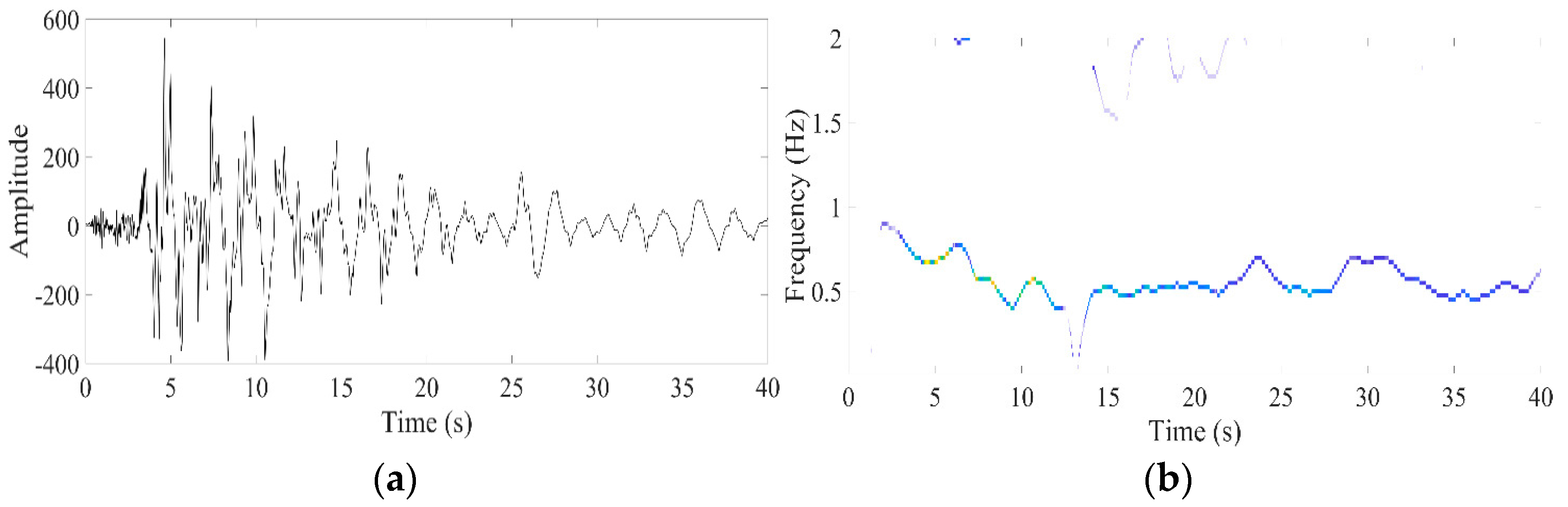
4.2.2. Seismic Data-2: Northridge Earthquake, 1994

A 10-story residential building was designed in 1974 in Northridge. Before the earthquake, four accelerometer sensors were installed on the first, fourth, and eighth floors of the building. Earthquake data were collected from the top floor of the building for approximately 60 s. Only the seismic signals for the first 25 s are analyzed because the remaining signals do not provide useful information. The time-domain representations of the signals and their LMSST responses could be seen in Figure 3a,b, respectively.
The pre-event frequency of the building was about 2 Hz, and during the seismic event, the frequency of the building kept fluctuating. The fluctuation in the building can be attributed to seismic events, ground motion, and other parameters related to the building. After the seismic event, the building tried to regain its pre-event frequency, but the building could not regain its natural frequency and a significant drop of around 25% can be observed. As a result, we can conclude that the building has sustained permanent structural damages due to the earthquake, as also reported on the website (http://www.strongmotioncenter.org/vdc/scripts/download_tar.plx, accessed on 4 April 2019).

4.2.3. Seismic Data-3: Northridge Earthquake, 1994

The seven-story Van Nuys Hotel was built in 1966. The hotel was lavishly outfitted with sensors on every floor. The time history data of the earthquake collected from the building’s roof, as well as the time–frequency responses obtained with the LMSST technique, are plotted in Figure 4a,b, respectively. From the figures, it can be observed that the pre-event frequency of the building was around 1 Hz, and during the earthquake, it gradually decreased down to 0.5 Hz. After the earthquake, the building tried to regain its pre-event frequency but could not achieve it. The post-event frequency dropped by almost 50%. Thus, it can be concluded that the building was permanently damaged by the earthquake, as also reported on the website (http://www.strongmotioncenter.org/vdc/scripts/download_tar.plx).

5. Conclusions

The health of the structure after any seismic event can be assessed by comparing its pre-event and post-event natural frequencies when there is no influence of external excitation (i.e., an earthquake). The amplitudes of the post-event and pre-event signals captured by sensors are relatively low compared to the signals captured during seismic events. Consequently, traditional TF methods such as WD, WVD, PWVD, SPWVD, and SST—which do not have concentrated TF planes—cannot detect the post-event and pre-event frequencies of the building. To overcome this problem, in this research, for the first time, a new TF method called LMSST was employed for post-earthquake damage detections. Through a multi-component synthetic signal, we have shown that it has the most concentrated TF plane and the best temporal frequency localization capability. Besides that, we have also analyzed the performance of LMSST for three different real-time recorded earthquake data sets and found that, unlike traditional methods, it can precisely and comprehensively detect the post and pre-event frequencies of the building. Thus, it was concluded that it is the most suitable TF method for the post-earthquake damage identifications of the buildings.

Author Contributions

Software, V.S.; Validation, V.S.; Formal analysis, R.K.; Writing—original draft, R.K. and V.S.; Writing—review & editing, V.S.; Supervision, M.I. All authors have read and agreed to the published version of the manuscript.

Funding

The APC was funded by Manipal Academy of Higher Education.

Conflicts of Interest

The authors declare no conflict of interest.

References

  1. Omoya, M.; Ero, I.; Zakir, E.M.; Burton, H.V.; Brandenberg, S.; Sun, H.; Yi, Z.; Kang, H.; Nweke, C.C. A relational database to support post-earthquake building damage and recovery assessment. Earthq. Spectra 2022, 38, 1549–1569. [Google Scholar] [CrossRef]
  2. Doebling, S.W.; Farrar, C.R.; Prime, M.B.; Shevitz, D.W. Damage Identification and Health Monitoring of Structural and Mechanical Systems from Changes in Their Vibration Characteristics: A Literature Review; LA—13070-MS, 249299; U.S. Department of Energy Office of Scientific and Technical Information: Oak Ridge, TN, USA, 1996. [Google Scholar] [CrossRef] [Green Version]
  3. Clinton, J.F. The observed wander of the natural frequencies in a structure. Bull. Seismol. Soc. Am. 2006, 96, 237–257. [Google Scholar] [CrossRef] [Green Version]
  4. Bradford, S.C.V. Time-Frequency Analysis of Systems with Changing Dynamic Properties. Ph.D. Thesis, California Institute of Technology, Pasadena, CA, USA, 2006. [Google Scholar] [CrossRef]
  5. Ozer, E.; Özcebe, A.G.; Negulescu, C.; Kharazian, A.; Borzi, B.; Bozzoni, F.; Molina, S.; Peloso, S.; Tubaldi, E. Vibration-based and near real-time seismic damage assessment adaptive to building knowledge level. Buildings 2022, 12, 416. [Google Scholar] [CrossRef]
  6. Cano, L.; Martínez-Cruzado, J.A. Damage identification of structures using instantaneous frequency changes. In Proceedings of the International Conference on Computational Methods in Structural Dynamics and Earthquake Engineering, Rethymno, Greece, 13–16 June 2007. [Google Scholar]
  7. Black, C.J.; Ventura, C.E. Joint time-frequency analysis of a 20 story instrumented building during two earthquakes. In Proceedings of the XVII International Modal Analysis Conference, Kissimee, FL, USA, 8–11 February 1999. [Google Scholar]
  8. Bradford, C.; Yang, J.; Heaton, T. Variations in the dynamic properties of structures: The Wigner-Ville distribution. In Proceedings of the 8th U.S. National Conference on Earthquake Engineering, Pasadena, CA, USA, 18–22 April 2006. [Google Scholar]
  9. Li, Y.; Zheng, X. Wigner-Ville distribution and its application in seismic attenuation estimation. Appl. Geophys. 2007, 4, 245–254. [Google Scholar] [CrossRef]
  10. Wu, X.; Liu, T. Spectral decomposition of seismic data with reassigned smoothed pseudo Wigner–Ville distribution. J. Appl. Geophys. 2009, 68, 386–393. [Google Scholar] [CrossRef]
  11. Michel, C.; Gueguen, P. Time-frequency analysis of small frequency variations in civil engineering structures under weak and strong motions using a reassignment method. Struct. Health Monit. 2010, 9, 159–171. [Google Scholar] [CrossRef] [Green Version]
  12. Liu, N.; Schumacher, T.; Li, Y.; Xu, L.; Wang, B. Damage detection in reinforced concrete member using local time-frequency transform applied to vibration measurements. Buildings 2023, 13, 148. [Google Scholar] [CrossRef]
  13. Kumar, R.; Sumathi, P.; Kumar, A. Synchrosqueezing transform-based frequency shifting detection for earthquake-damaged structures. IEEE Geosci. Remote Sens. Lett. 2017, 14, 1393–1397. [Google Scholar] [CrossRef]
  14. Yu, G.; Wang, Z.; Zhao, P.; Li, Z. Local maximum synchrosqueezing transform: An energy-concentrated time-frequency analysis tool. Mech. Syst. Signal Process. 2019, 117, 537–552. [Google Scholar] [CrossRef]
  15. Qian, S.; Chen, D. Joint time-frequency analysis. IEEE Signal Process. Mag. 1999, 16, 52–67. [Google Scholar] [CrossRef]
  16. Kumar, R.; Zhao, W.; Singh, V. Joint time-frequency analysis of seismic signals: A critical review. Struct. Durab. Health Monit. 2018, 12, 65–83. [Google Scholar]
  17. Cohen, L. Time-frequency distributions-a review. Proc. IEEE 1989, 77, 941–981. [Google Scholar] [CrossRef] [Green Version]
  18. Staszewski, W.J.; Robertson, A.N. Time-frequency and time-scale analyses for structural health monitoring. Philos. Trans. R. Soc. A Math. Phys. Eng. Sci. 2007, 365, 449–477. [Google Scholar] [CrossRef] [PubMed]
  19. Yan, Y.; Poon, C.C.; Zhang, Y. Reduction of motion artifact in pulse oximetry by smoothed pseudo Wigner-Ville distribution. J. NeuroEng. Rehabil 2005, 2, 3. [Google Scholar] [CrossRef] [PubMed] [Green Version]
  20. Daubechies, I.; Lu, J.; Wu, H.-T. Synchrosqueezed wavelet transforms: An empirical mode decomposition-like tool. Appl. Comput. Harmon. Anal. 2011, 30, 243–261. [Google Scholar] [CrossRef] [Green Version]
  21. Herrera, R.H.; Tary, J.B.; van der Baan, M.; Eaton, D.W. Body wave separation in the time-frequency domain. IEEE Geosci. Remote Sens. Lett. 2015, 12, 364–368. [Google Scholar] [CrossRef]
  22. Tary, J.B.; Herrera, R.H.; van der Baan, M. The synchrosqueezing transform for high-resolution time-frequency representation of microseismic recordings. In Proceedings of the 75th EAGE Conference and Exhibition Incorporating SPE EUROPEC 2013, London, UK, 10–13 June 2013. [Google Scholar] [CrossRef]
  23. Kumar, R.; Zhao, W. Predominant frequency detection of seismic signal based on Gabor–Wigner transform for earthquake early warning systems. Asian J. Civ. Eng. 2018, 19, 927–936. [Google Scholar] [CrossRef]
  24. Kumar, R.; Zhao, W. Theory and applications of time-frequency methods for analysis of non-stationary vibration and seismic signal. In Proceedings of the 2nd International Conference on Vision, Image and Signal Processing, Las Vegas, NV, USA, 27–29 August 2018; pp. 1–6. [Google Scholar] [CrossRef]
  25. Saldana, C.L. On Time-Frequency Analysis for Structural Damage Detection. Ph.D. Thesis, University of Puerto Rico, San Juan, PUR, USA, June 2014. [Google Scholar]
  26. Aviyente, S.; Williams, W.J. Minimum entropy time-frequency distributions. IEEE Signal Process. Lett. 2005, 12, 37–40. [Google Scholar] [CrossRef]
  27. Yu, G.; Yu, M.; Xu, C. Synchroextracting transform. IEEE Trans. Ind. Electron. 2017, 64, 8042–8054. [Google Scholar] [CrossRef]
  28. Boashash, B.; Black, P.J. An efficient real-time implementation of the Wigner-Ville distribution. IEEE Trans. Acoust. Speech Signal Process. 1987, 35, 1611–1618. [Google Scholar] [CrossRef]
  29. Creed, S.G. Assessment of Large Engineering Structures Using Data Collected during In-Service Loading in Structural Assessment; Butterworths and Company Publishers, Limited: Singapore, 1987. [Google Scholar]
Figure 1. Frequencytime curves: (a) synthetic signal with five components; (b) WD; (c) WVD; (d) PWVD; (e) SPWVD; (f) SST; (g) LMSST.
Buildings 13 01614 g001
Figure 2. Frequencytime curves: (a) time domain representation of seismic dat−1; (b) WD; (c) WVD; (d) PWVD; (e) SPWVD; (f) SST; (g) LMSST.
Buildings 13 01614 g002
Figure 3. Time domain representations: (a) seismic data−2; (b) the corresponding LMSST.
Buildings 13 01614 g003
Figure 4. Time domain representations: (a) seismic data−3; (b) corresponding LMSST.
Buildings 13 01614 g004
Table 1. Renyi entropy measures of various TF method for given synthetic signal.
Time–Frequency MethodsRenyi Entropy
Test Signal-1
WD18.278
WVD17.190
PWVD16.132
SPWVD15.613
SST11.020
LMSST10.910
Table 2. Details of the damaged buildings.
ParametersData-1Data-2Data-3
Earthquake, yearSan Fernando earthquake, 1971Northridge earthquake, 1994Northridge earthquake, 1994
Magnitude6.66.76.7
Epicenter31 km21 km18 km
Name of buildingsMillikan Library, Pasadena, USTen-story inhabited building, Burbank, USSeven-story Van Nuys hotel
Sensor’s positionEW roofRoof-centerRoof
Sampling frequency50 Hz50 Hz50 Hz
Peak acceleration340.8 cm/s2511.99 cm/s2550.22 cm/s2
Table 3. Renyi entropy measures of various TF method for Data-1.
Time–Frequency MethodsRenyi Entropy
Data-1 San-Fernando Earthquake, 1971
WD17.256
WVD15.980
PWVD15.816
SPWVD15.444
SST12.797
LMSST10.797
Disclaimer/Publisher’s Note: The statements, opinions and data contained in all publications are solely those of the individual author(s) and contributor(s) and not of MDPI and/or the editor(s). MDPI and/or the editor(s) disclaim responsibility for any injury to people or property resulting from any ideas, methods, instructions or products referred to in the content.

