
Climate Zoning for Buildings: From Basic to Advanced Methods—A Review of the Scientific Literature

Abstract
:1. Introduction
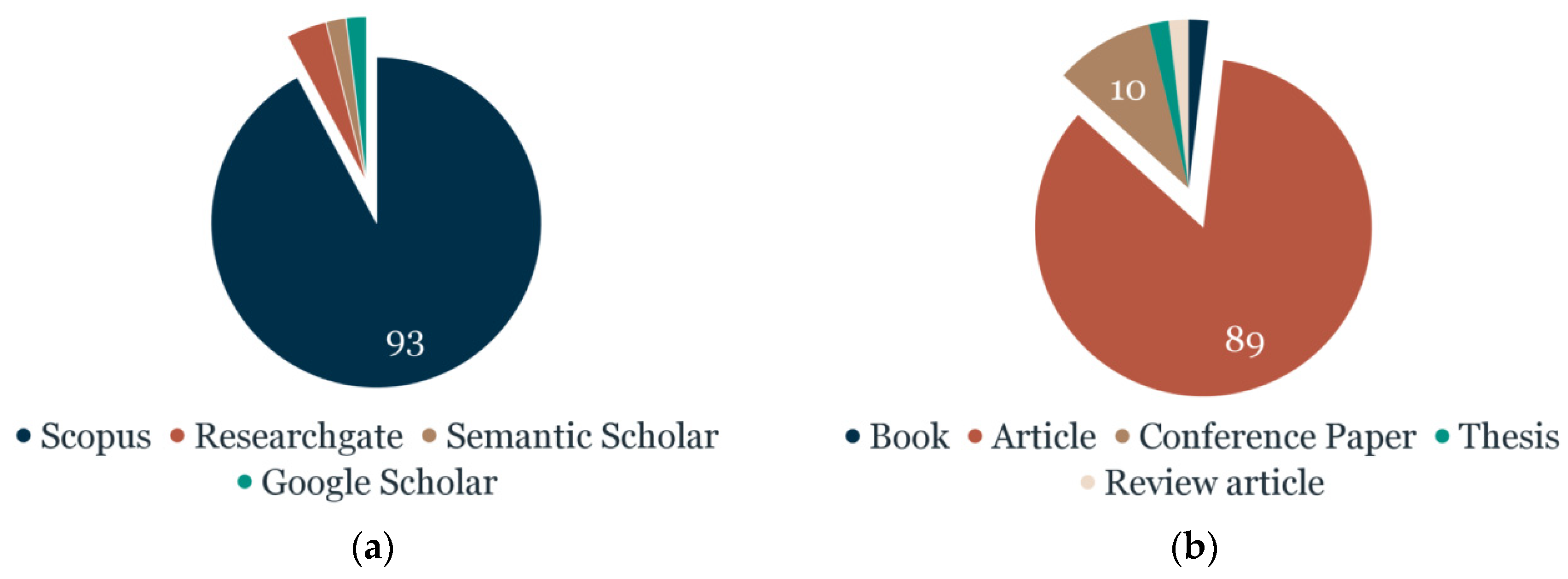
- The information on the CZB from scientific publications in 37 countries and 95 affiliations was collected and reviewed. The Scopus database was selected as a primary source of publications. Research articles represent 84% of the materials we analyzed, while conference papers account for 10%;
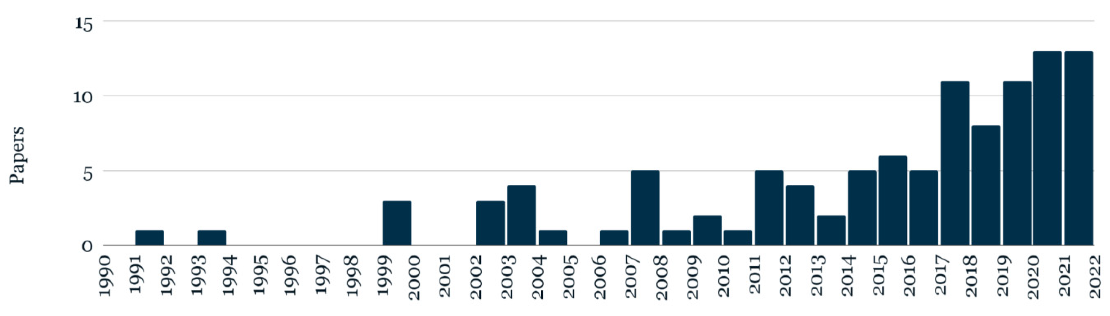
- This study is state-of-the-art since 51% of the publications reviewed were published between 2017 and 2022;
- The study essentially differentiates buildings’ CZ variables and buildings’ CZ methods, which were typically bundled in previously published works. Each of the categories was extensively reviewed and analyzed;
- An organized categorization of the most commonly used building CZ variables and building CZ methods (with criteria used in determining each method) is presented. The most commonly used CZB methods were evaluated emphasizing their similarities and differences, as well as their essential components and advantages. The current development of this field was explored and traced;
- Several additional machine learning (ML) methods for CZB have been revealed. In light of this, the category of conventional clustering techniques was expanded and given a new term, “Machine Learning Methods” (MLM). Additionally, a previously rare term, “The Interval Judgment Method” (IJM), has been put into use;
- Covering the gaps of prior works and concentrating on information that was not previously published, the primary sources of climate data and the form in which climate data are commonly used were recognized. The data on climate observation periods for CZB methods were also collected and analyzed. Other details such as the most commonly used software for energy simulations and the number of archetypes were mentioned;
- All collected data are shown in the condensed table with the following extracted features: sources, publication years, authors, publication type, country or region of study, CZ methods used, their number and combinations, number of climate zones, etc.
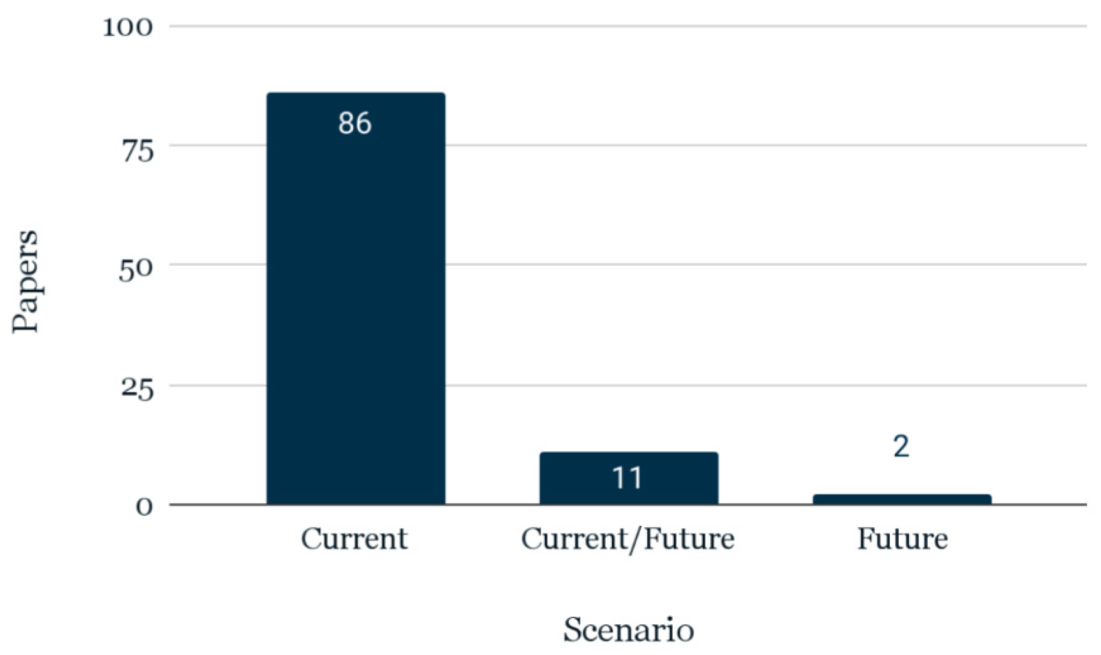
- Several promising studies regarding future climate scenarios in CZB were identified. In this review, 12% of publications dealt with future CZ, and their main principles are given;
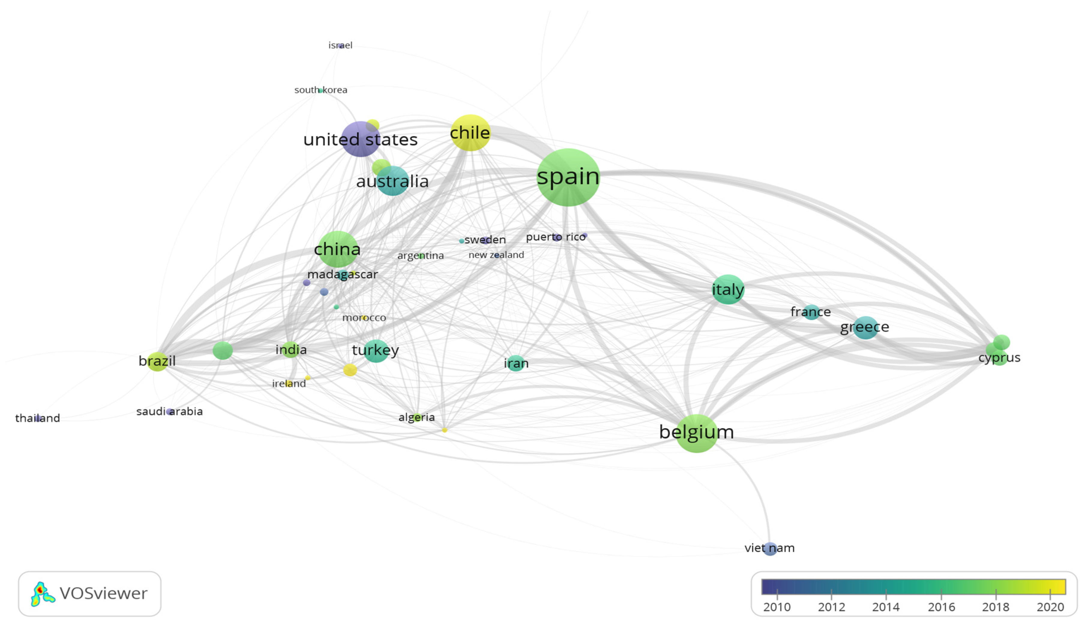
- Using bibliometric and bibliographic analysis for evaluating and analyzing the performance of research activities, this paper indicates substantially contributing authors, nations, the co-citation and bibliographic coupling networks, the direct citation network, etc.
2. Brief Historical Background of Climatic Zoning and Its Purpose
3. Methodology
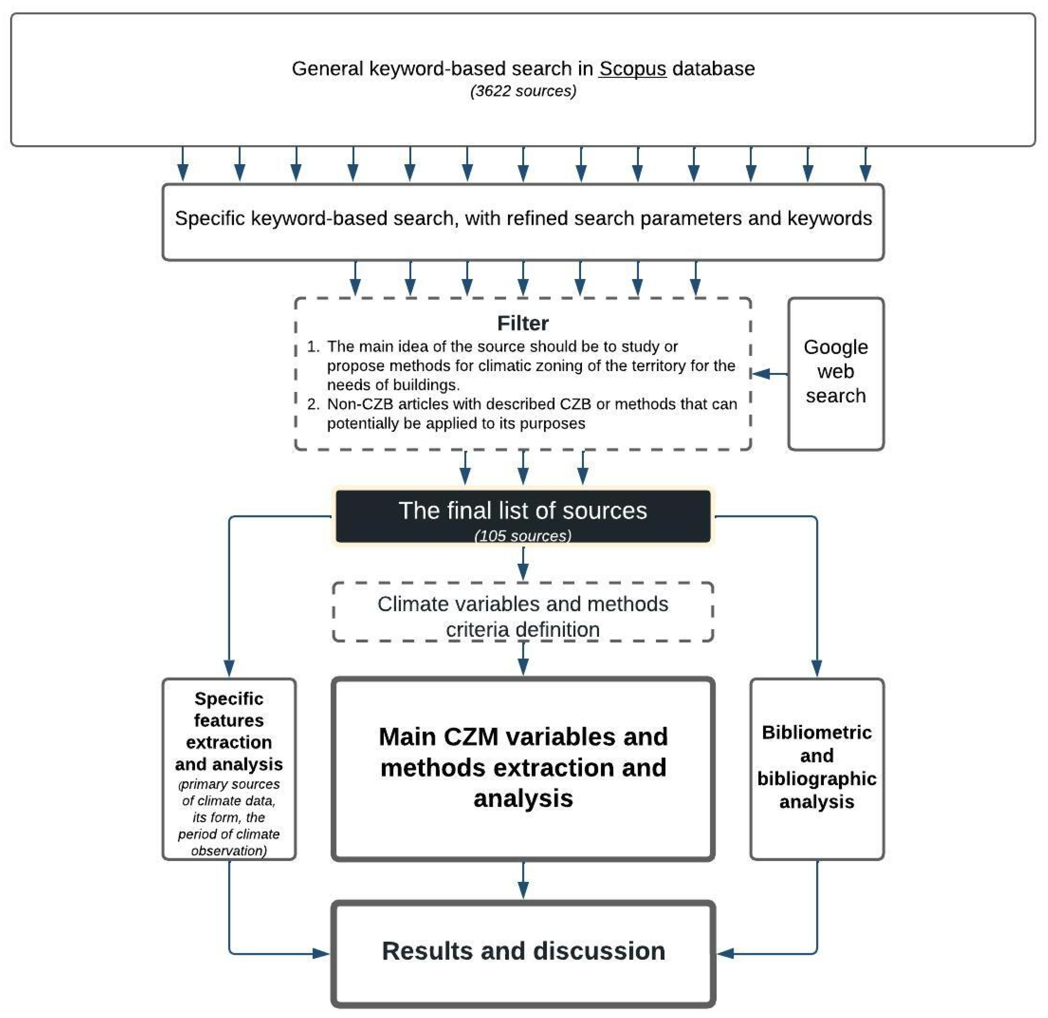
3.1. Literature Review Framework
- General keyword-based search in Scopus database;
- Specific keyword-based search, with refined search parameters and keywords to find the most relevant sources;
- The composition of the final list of sources using the following criteria. The main idea of the source should be to study or propose methods for climatic zoning of the territory for the needs of energy-efficient buildings or a non-CZB article with described methods which influence CZB or can potentially be applied to its purposes;
- Identifying and screening additional articles. The sources that were cited by an article from the shortlist became additional candidate sources. Relevant sources outside of Scopus were also identified by Google web search. Further, the candidate sources were checked following the established criteria, and the selected ones were added to the final list;
- Criteria were established to distinguish between climate variables and CZB methods;
- The review of each source and extraction of information on climate variables and CZB methods. Specific features (more details are included in the Data Collection section) were also extracted from the sources at this stage;
- All data were subjected to in-depth quantitative analysis (descriptive analysis);
- Sources cited in Scopus were subjected to basic bibliometric and bibliographic analysis to identify bibliometric networks;
- Discussion (interpretations of the findings, directions for future research, recommendations).
3.2. Adopted Bibliometric and Bibliographic Analysis
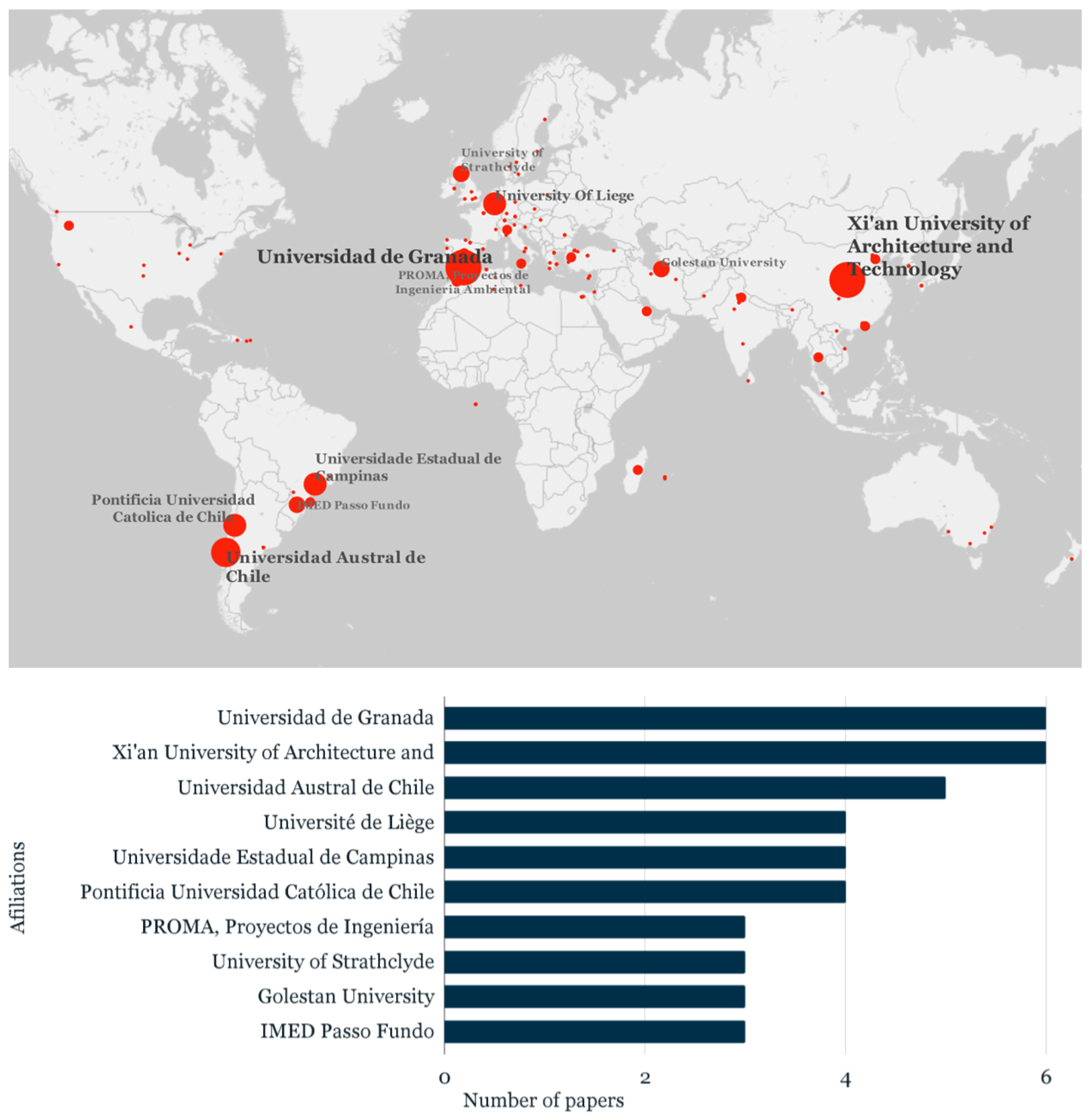
- A map of affiliations or public organizations which publish more articles than others in a CZB research field;
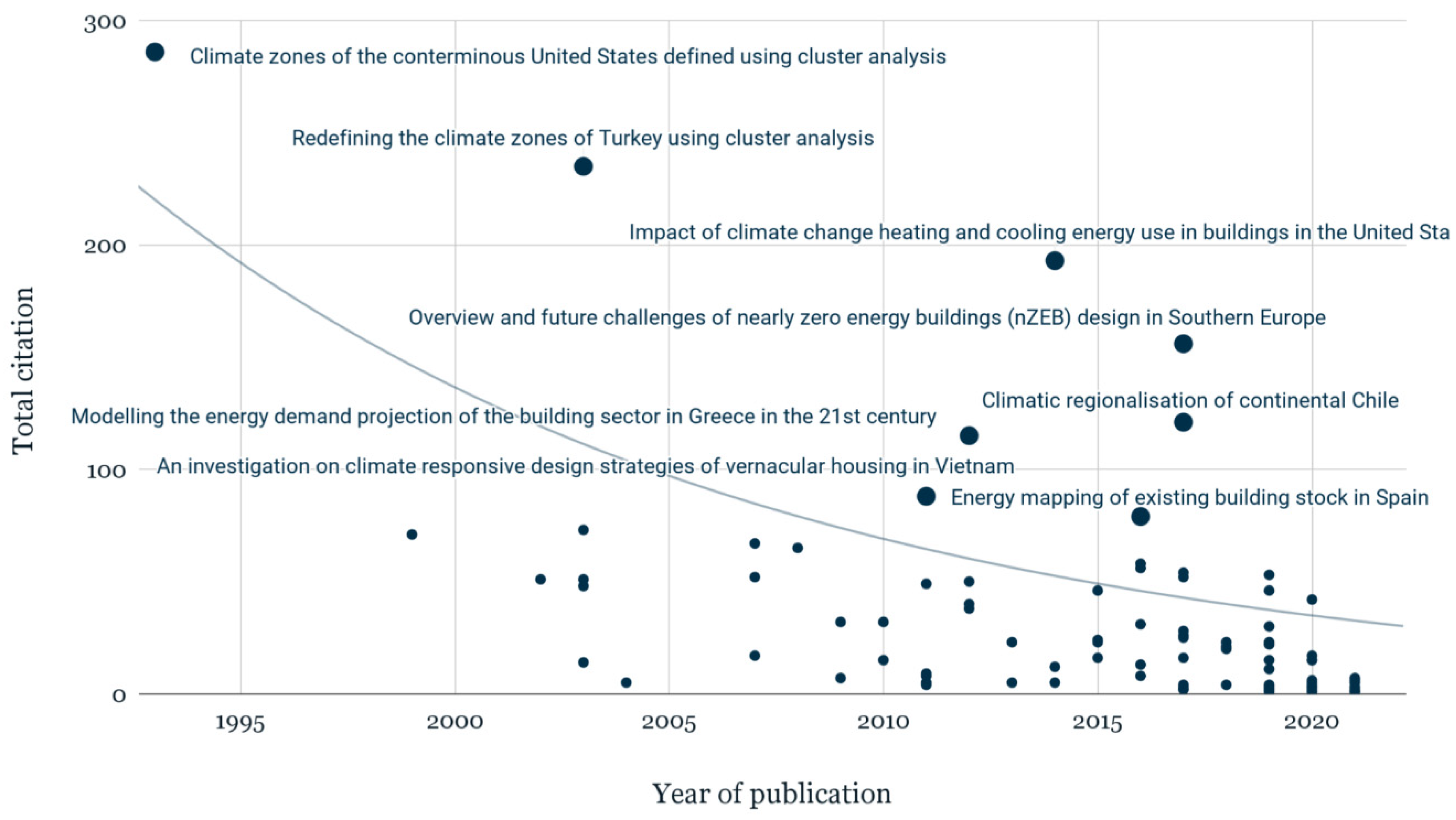
- The top 10 most cited articles;
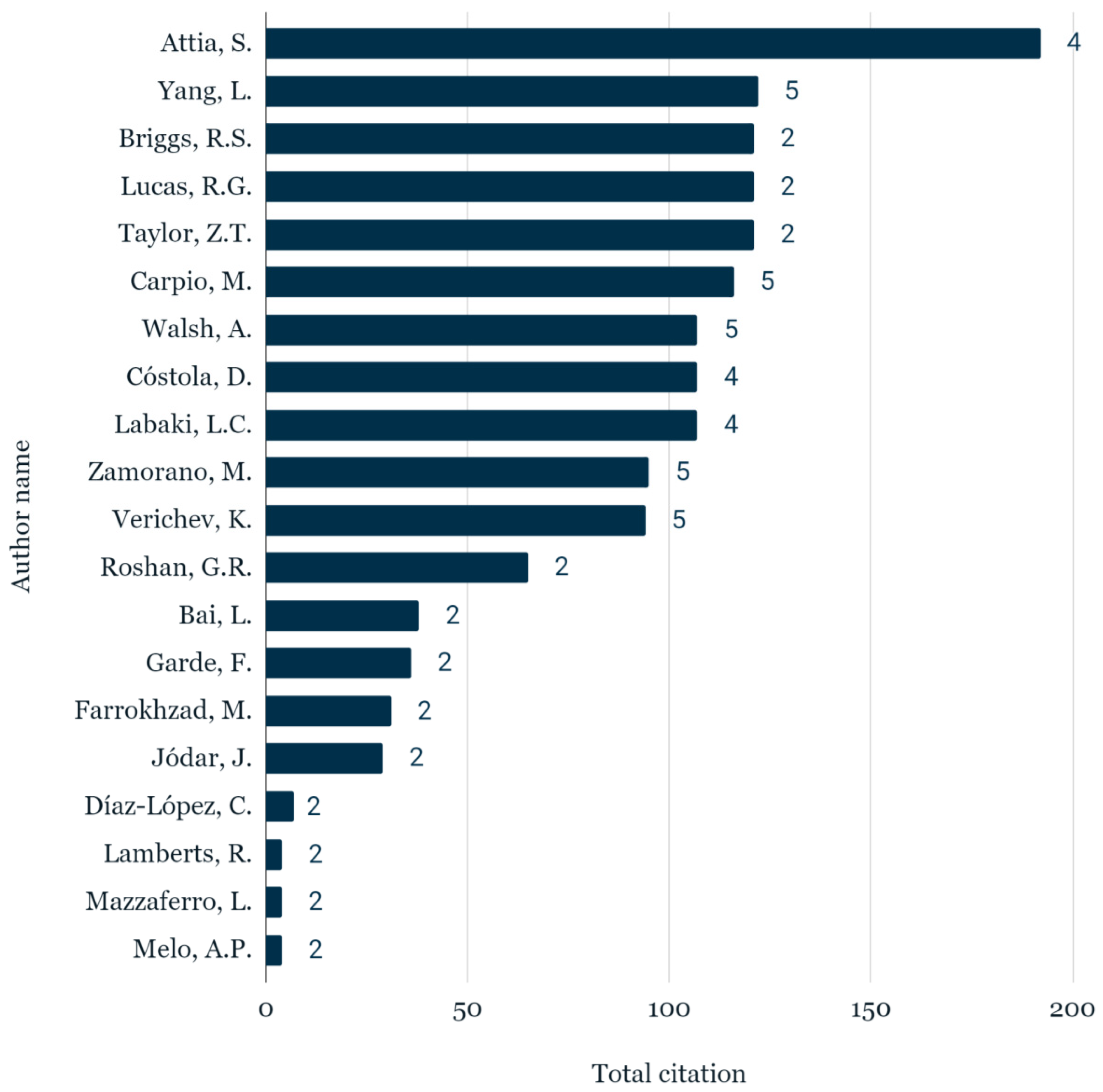
- The most contributing authors in the CZB area;
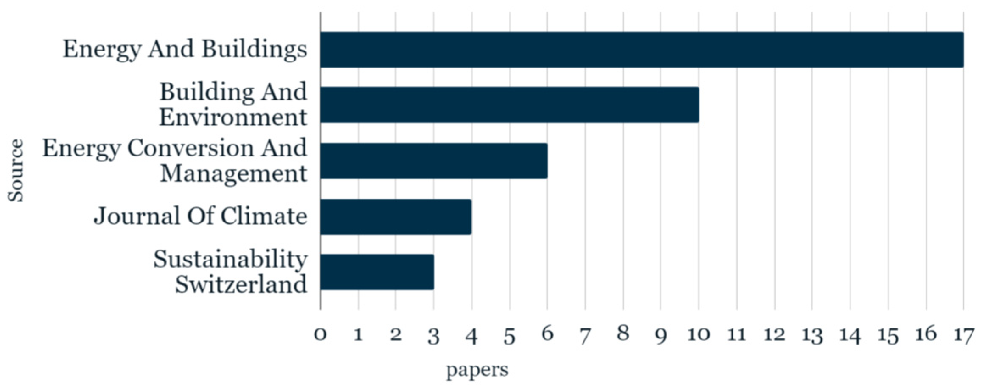
- The most popular journals for CZB;
- Citation over time analysis;
- The co-citation networks of researchers;
- The bibliographic coupling network of the top 100 authors;
- A direct citation network;
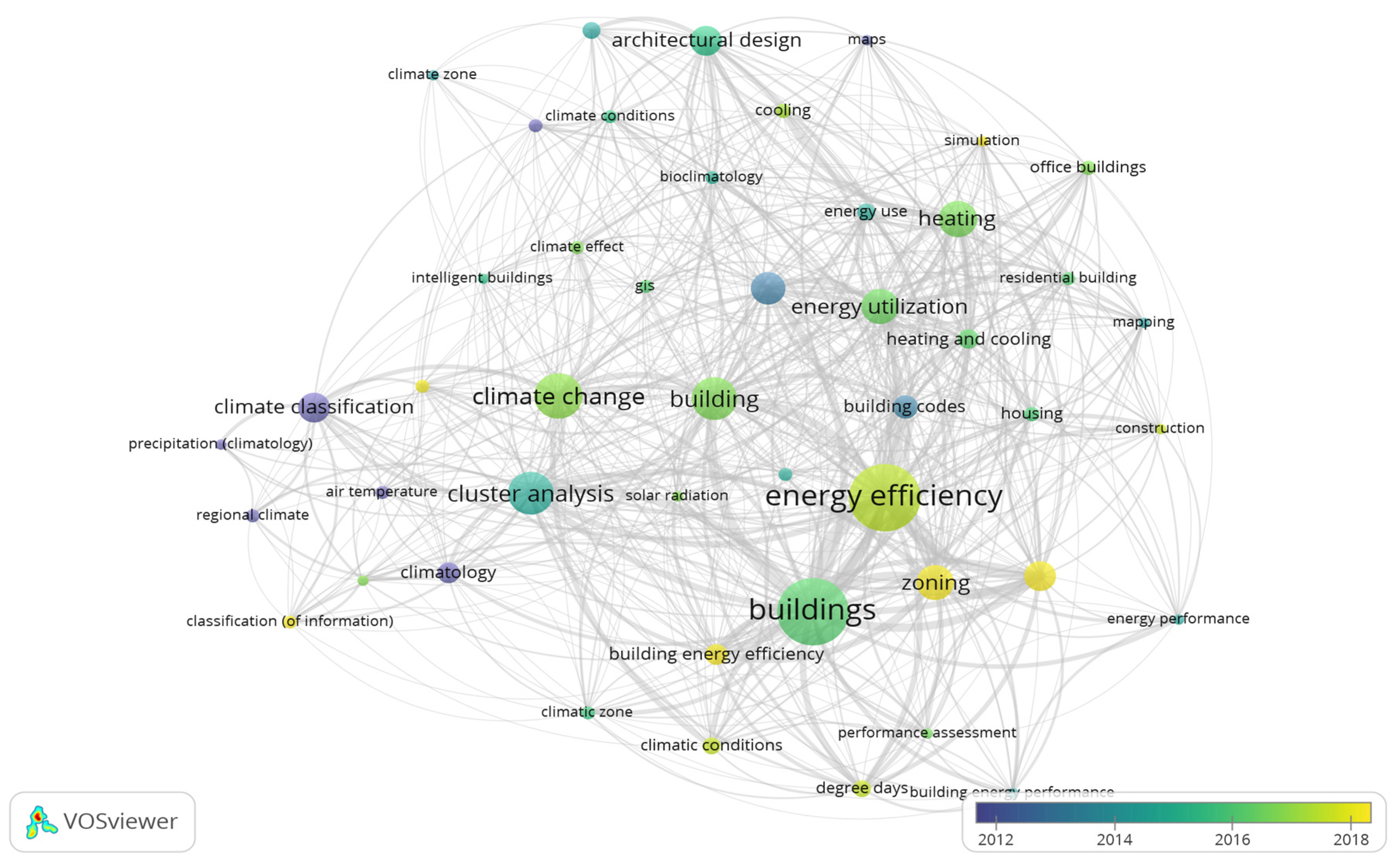
- The network of co-occurrences of keywords;
- The bibliometric coupling network of countries.
4. Data Collection
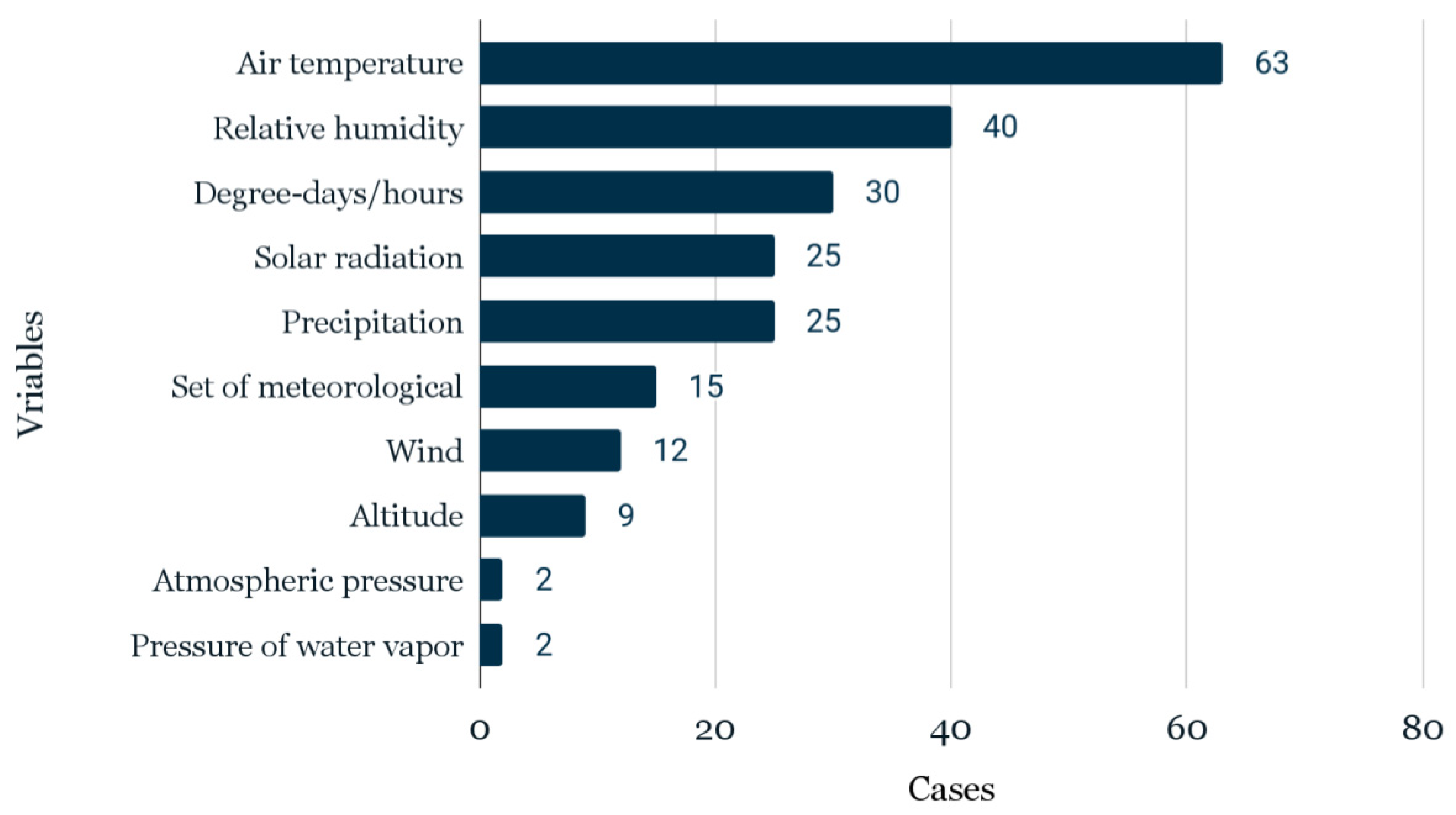
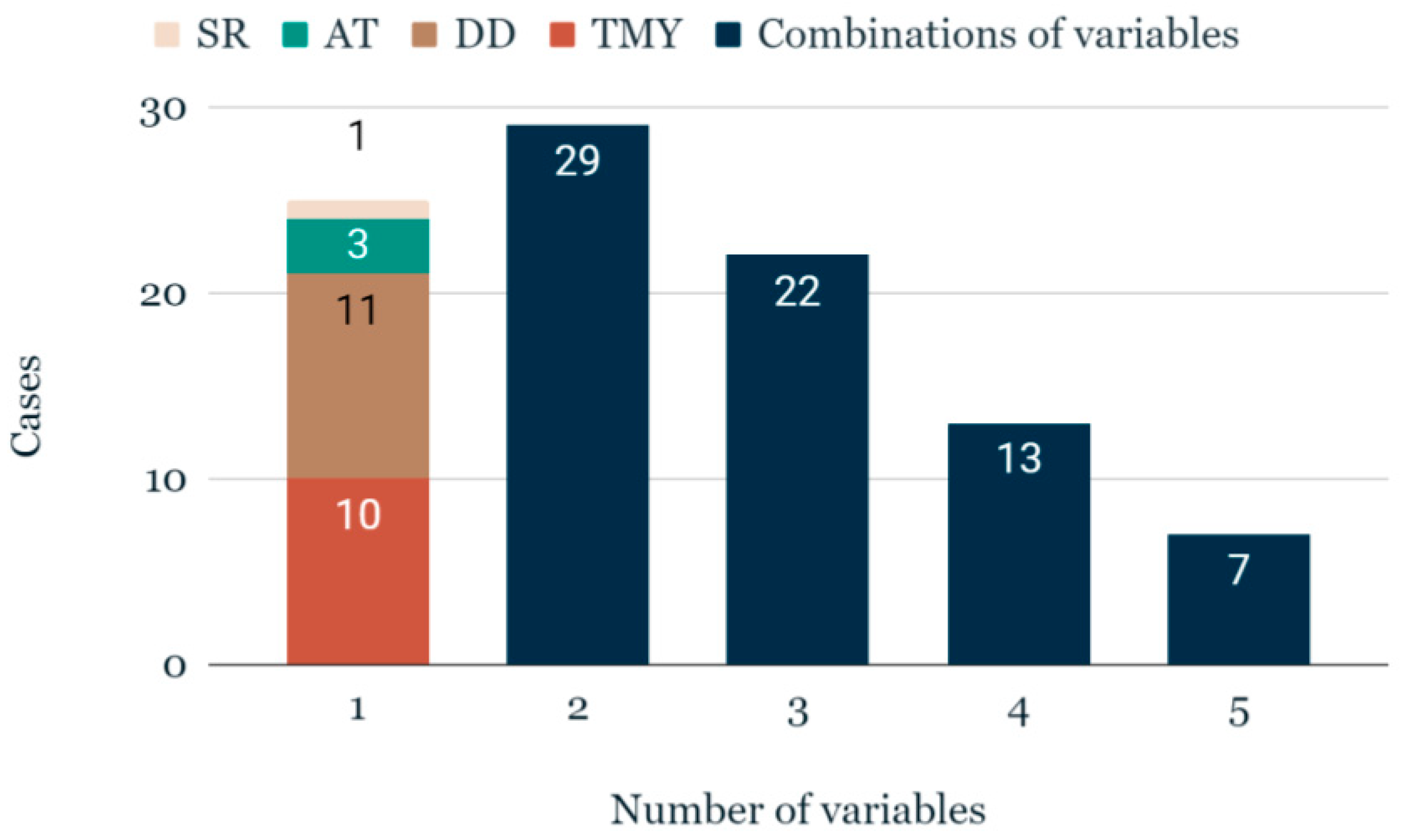
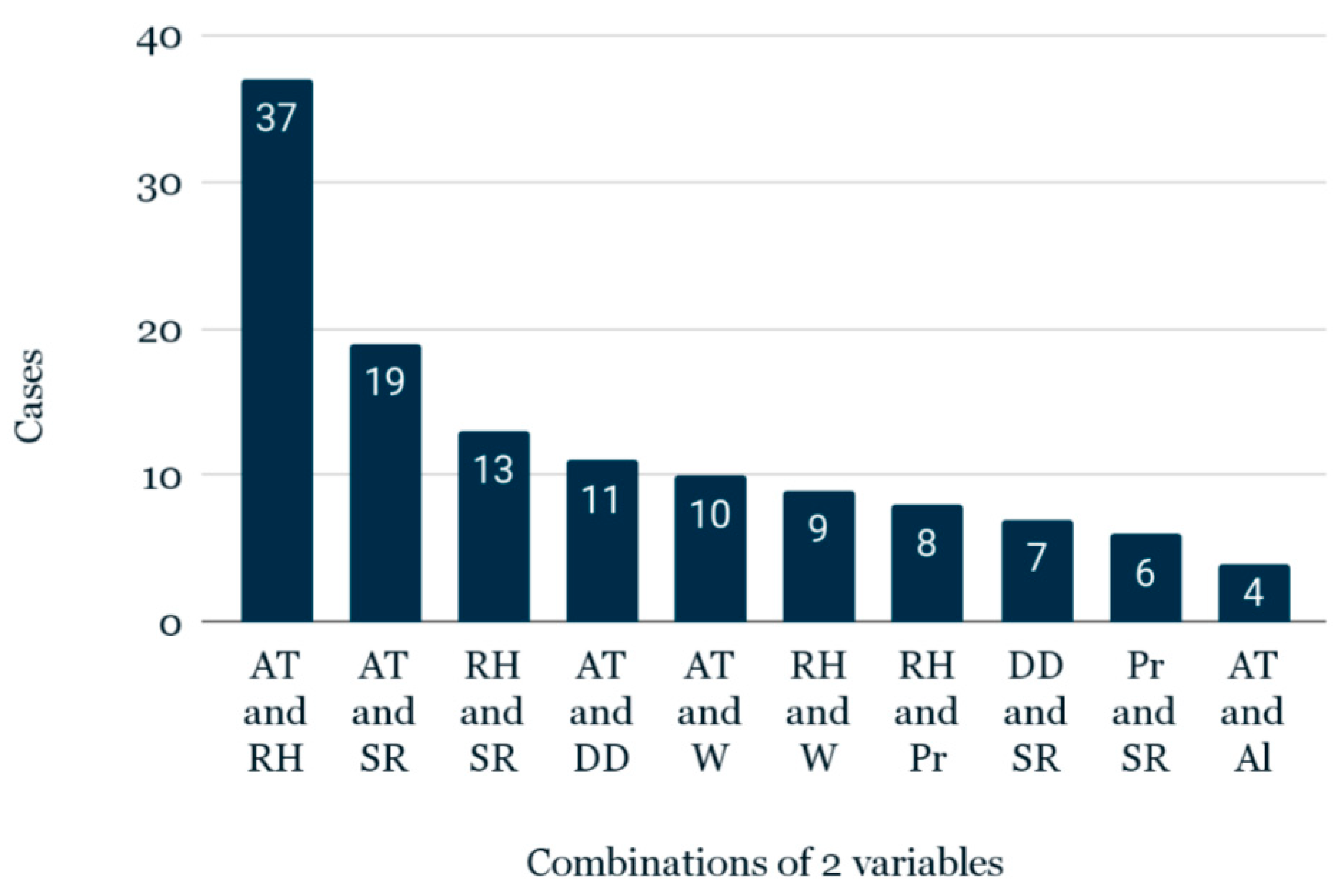
5. Climate Variables Used for CZB
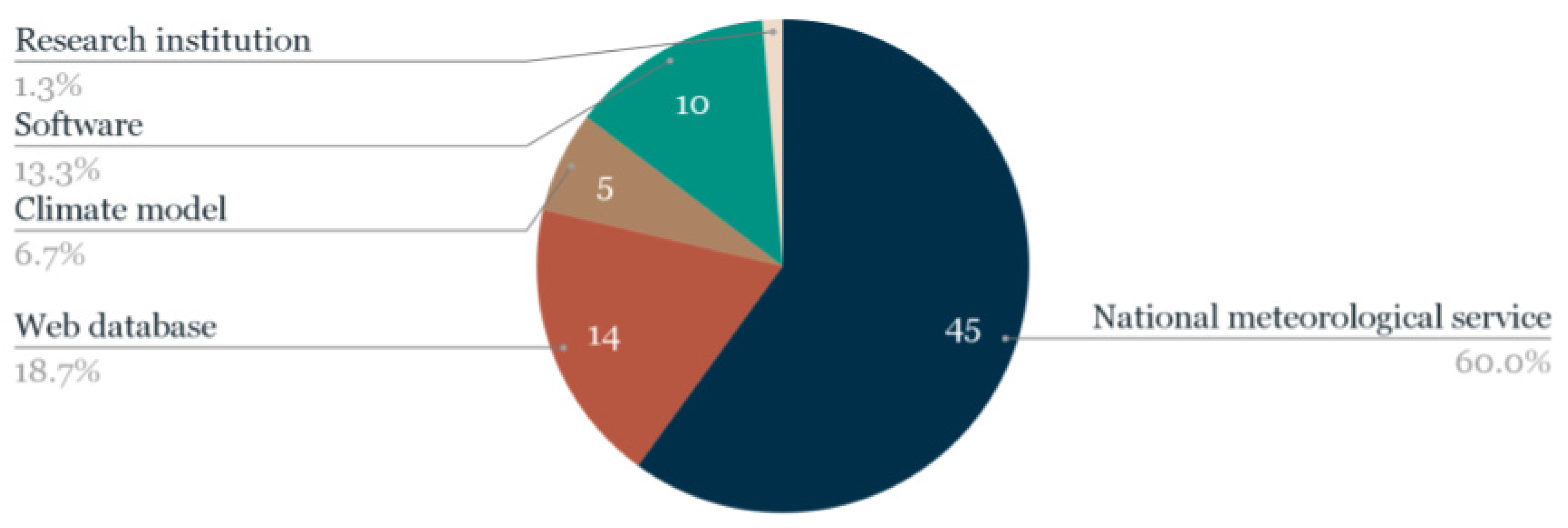
6. Climate Data Sources
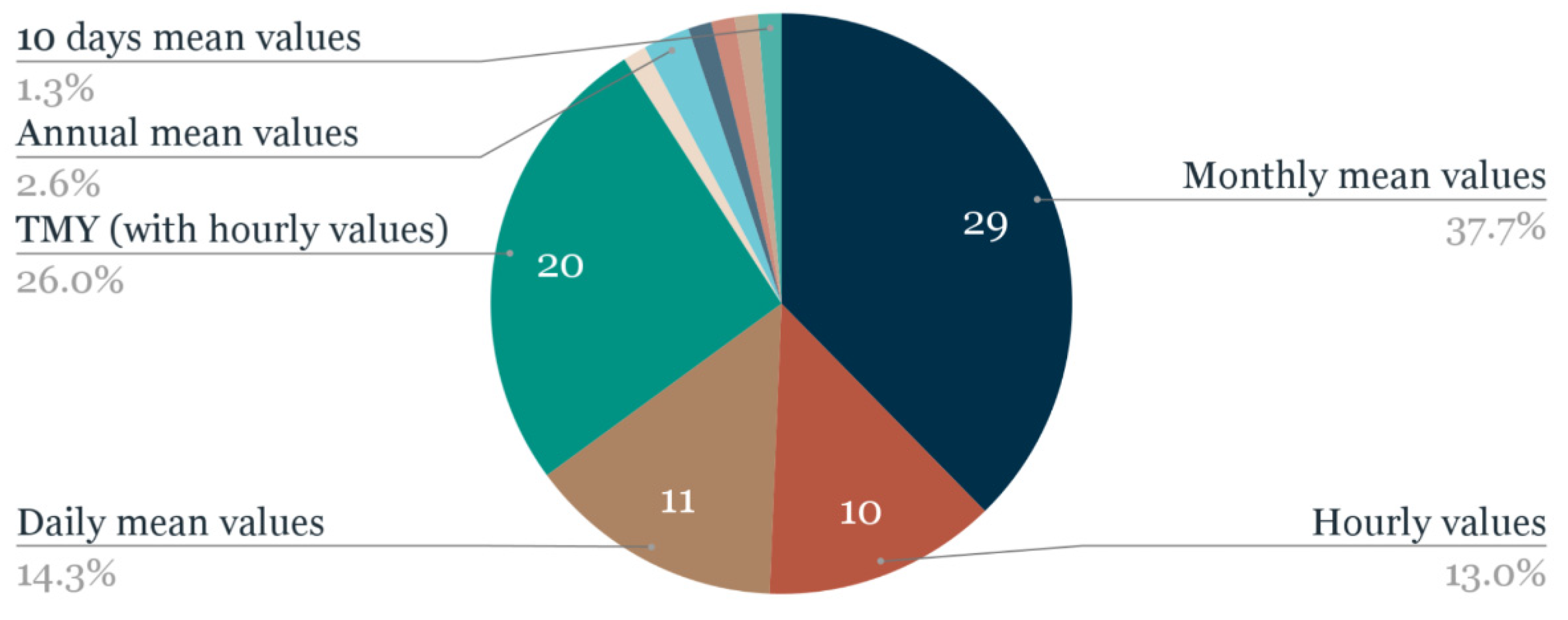
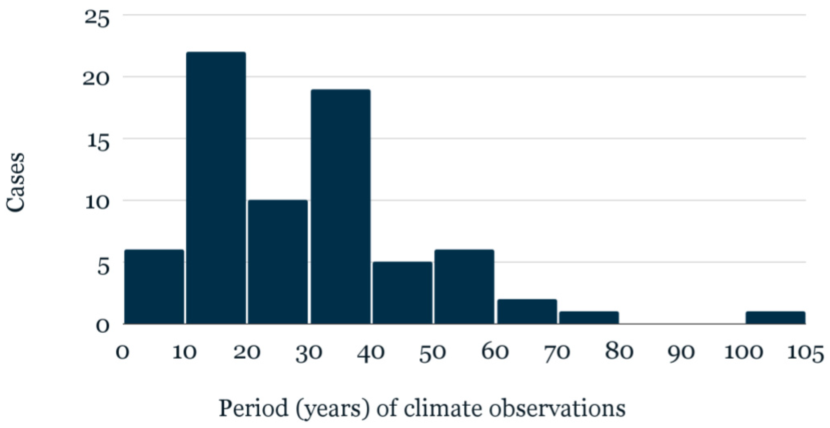
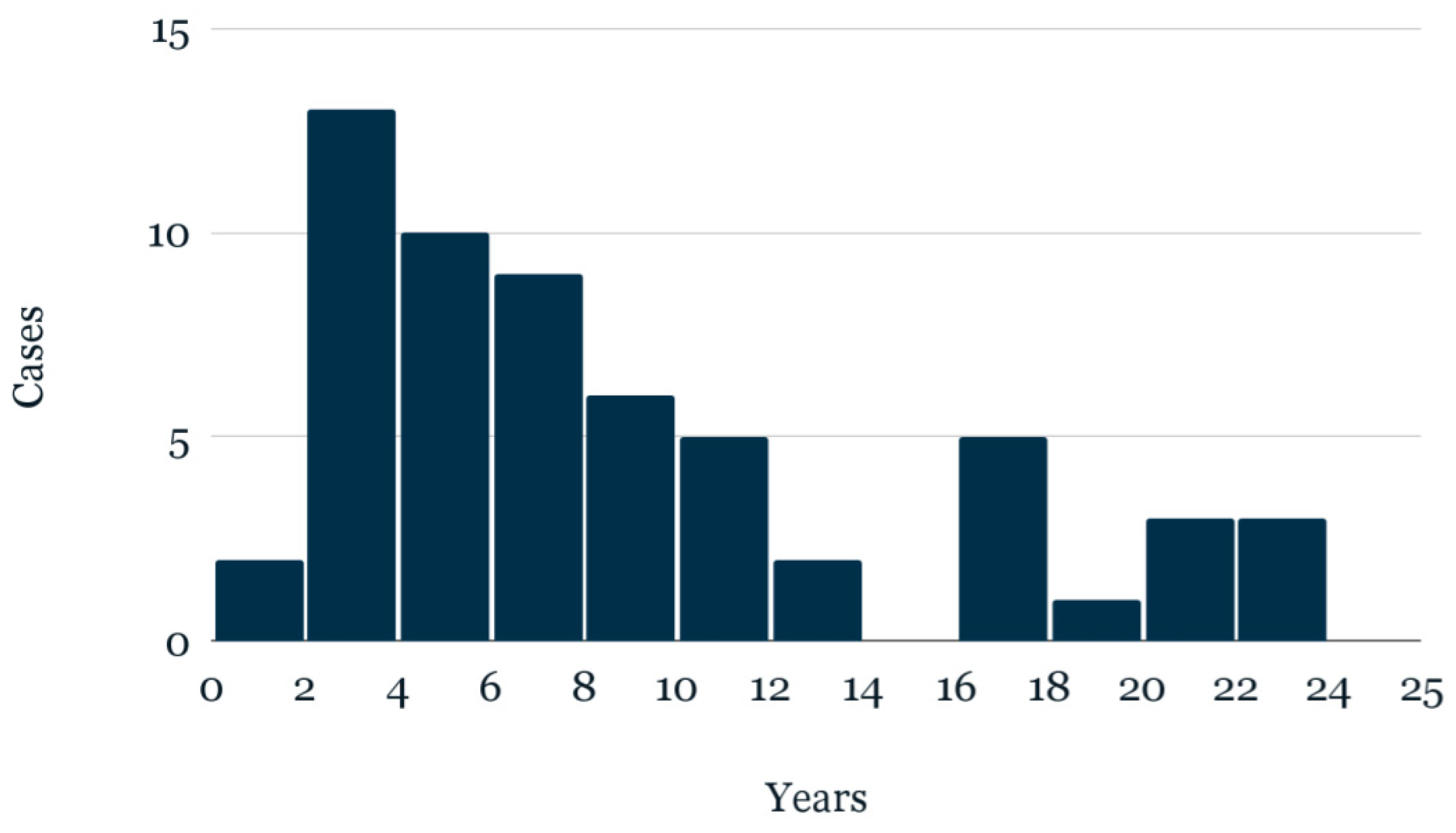
7. Period of Climate Observation
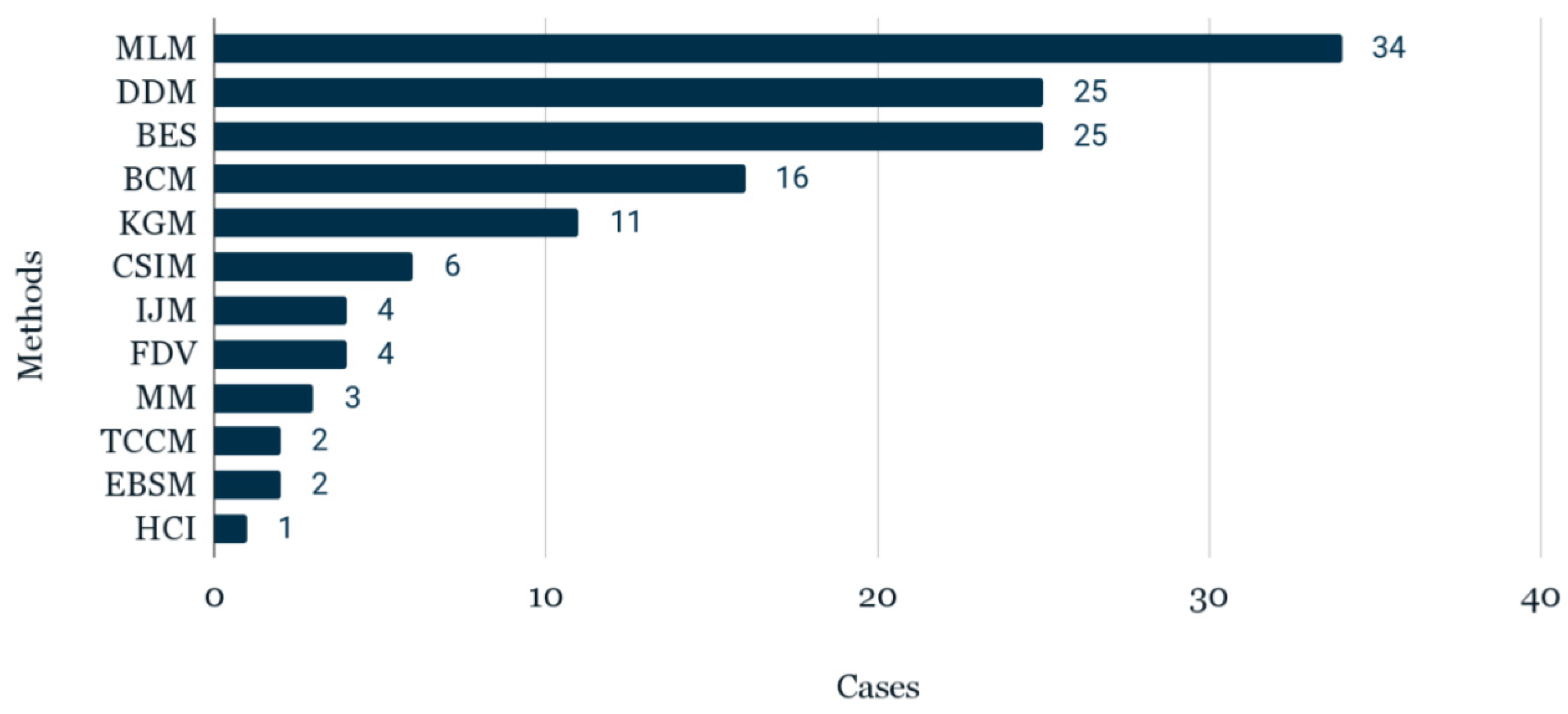
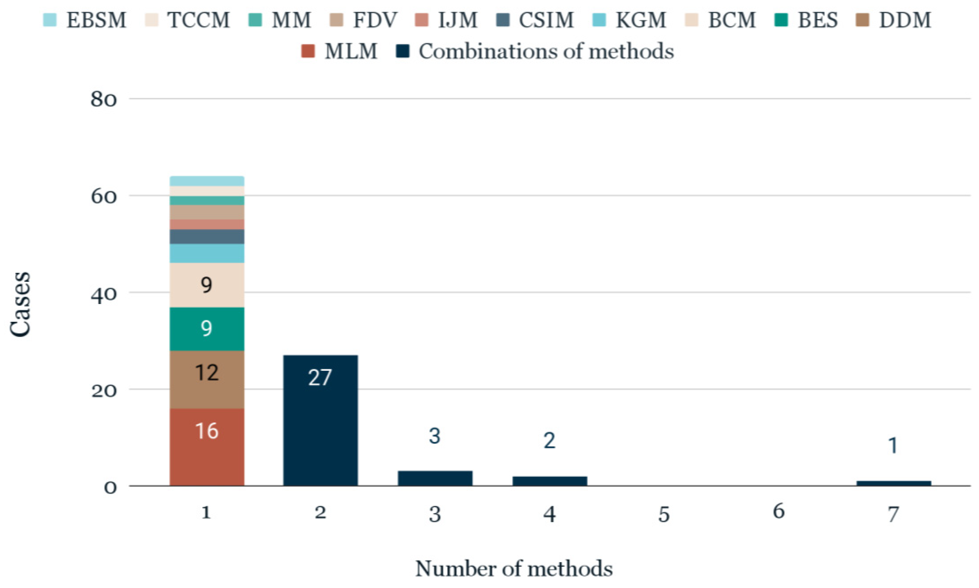
8. Methods Used for CZB
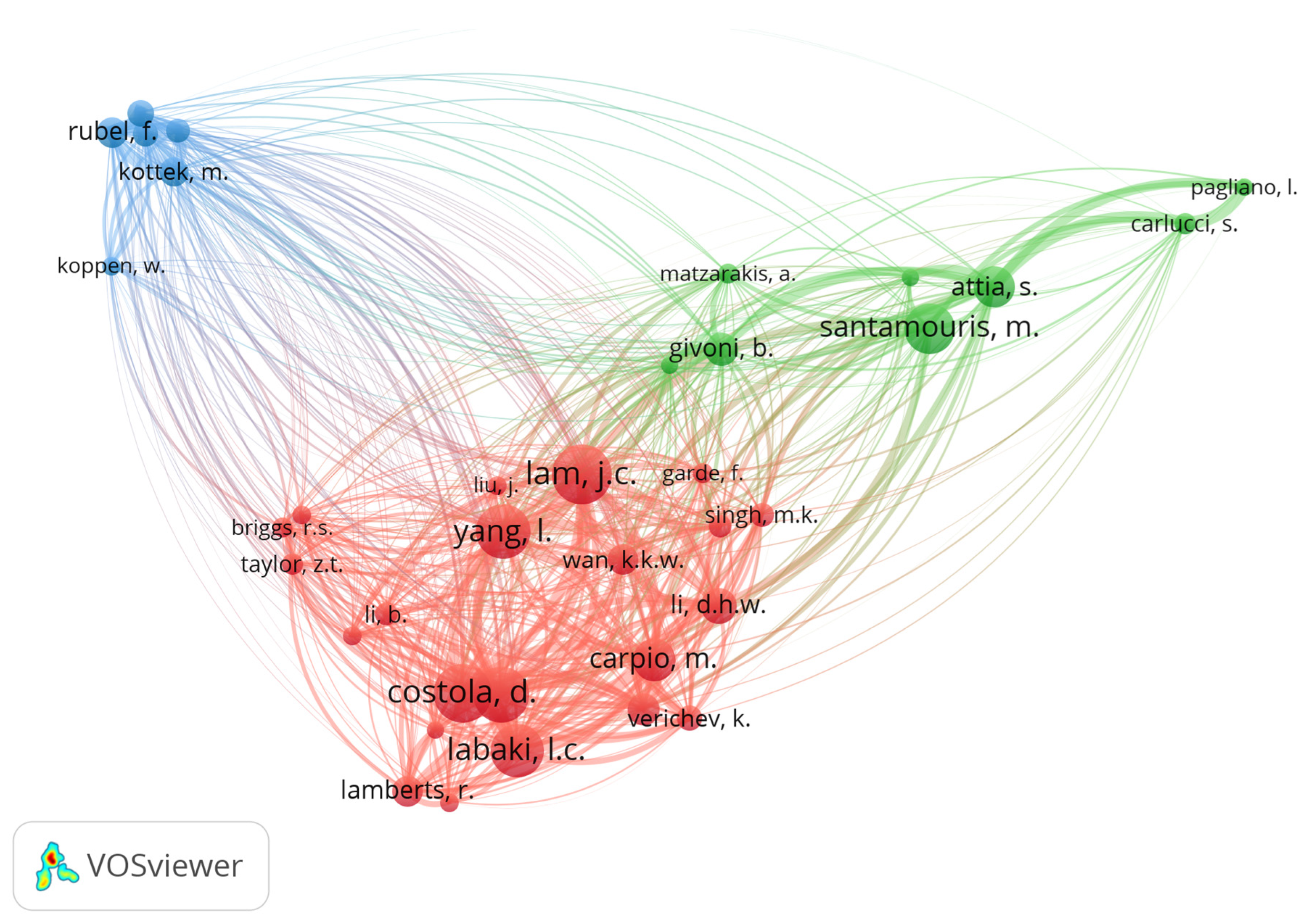
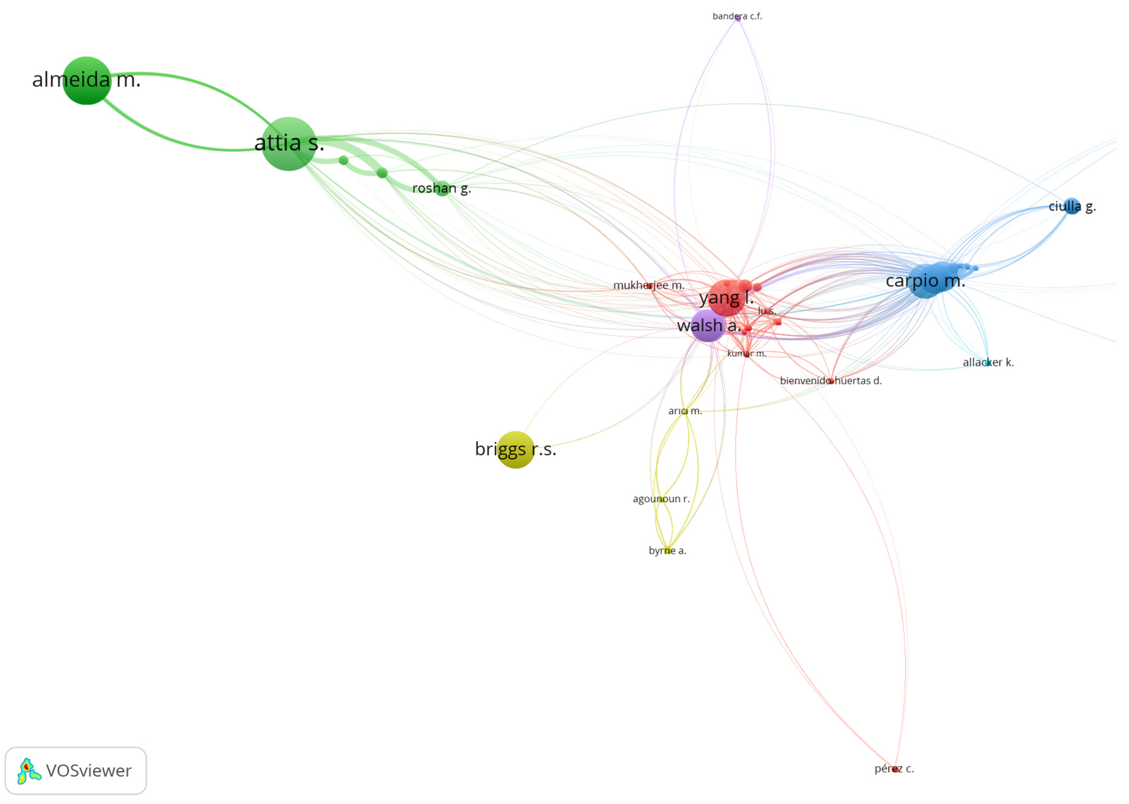
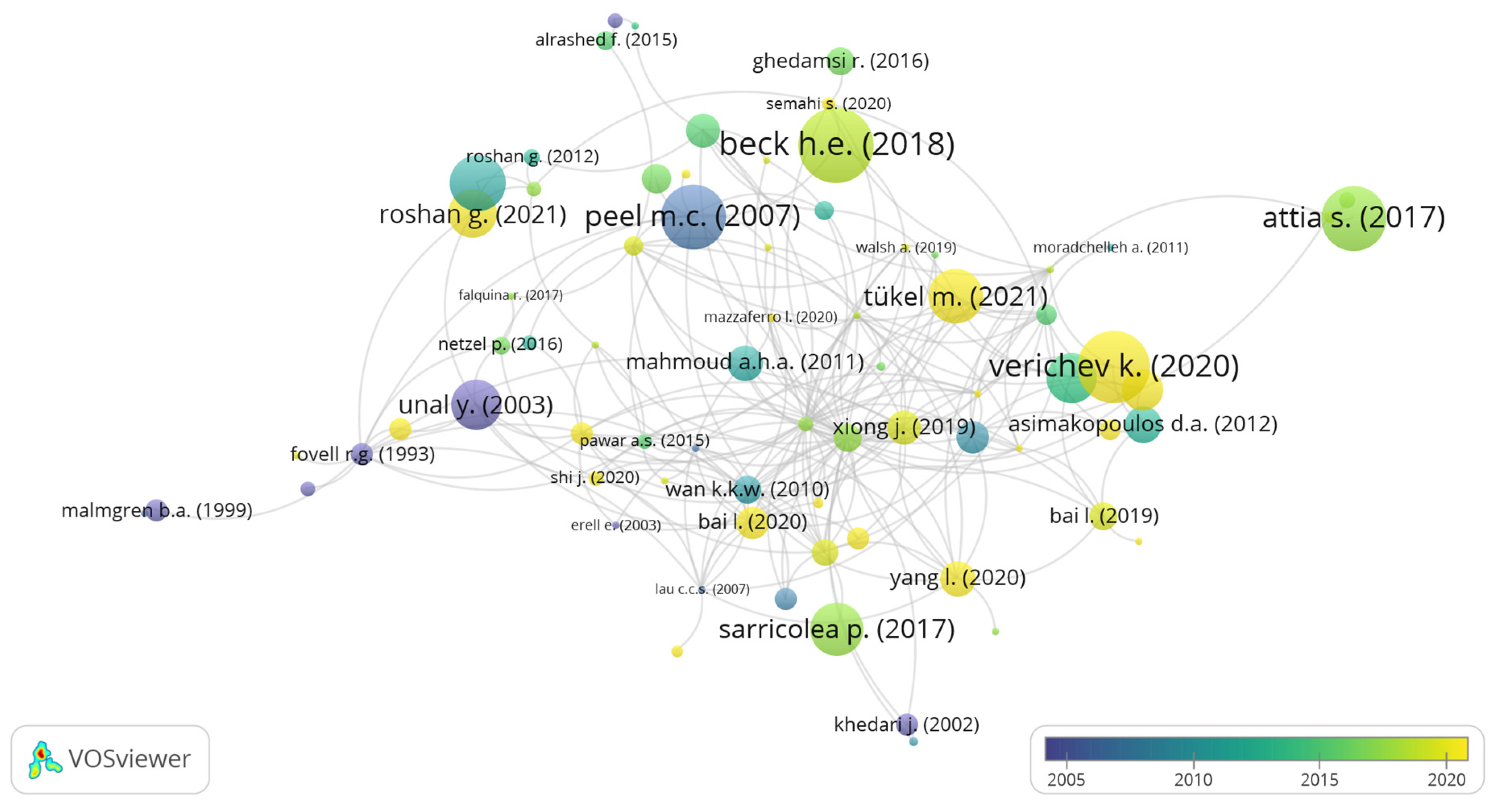
9. Bibliometric Analysis
10. Bibliographic Analysis
- Yang, L. and Walsh, A;
- Almeida, M., Attia, S., and Roshan, G.;
- Carpio, M., Verichev, K., and Diaz Lopez, C.
11. Discussion
12. Conclusions
Author Contributions
Funding
Data Availability Statement
Conflicts of Interest
Abbreviations
| Al | Altitude |
| AP | Atmospheric Pressure |
| ASHRAE | The American Society of Heating, Refrigerating, and Air-Conditioning Engineers |
| AT | Air Temperature |
| BCM | Bioclimatic Charts Method |
| BES | Building Energy Simulation |
| CA | Cluster Analysis |
| CSIM | Climate Severity Index Method |
| CDD | Cooling Degree-Day |
| CDH | Cooling Degree-Hour |
| CZ | Climatic Zoning |
| CZB | Climatic Zoning For Buildings |
| DBT | Dry-Bulb Temperature |
| DDs | Degree-Days |
| DHs | Degree-Hours |
| DDM | Degree-Days Methods |
| EBSM | Existing Building Stock Performance Method |
| FDV | A Frequency Distribution Of Climate Variables |
| GHG | Greenhouse Gas |
| GHI | Global Horizontal Irradiation |
| HCI | Heating Or Cooling Index |
| HC | Hierarchical Clustering |
| HDD | Heating Degree-Day |
| HDH | Heating Degree-Hour |
| HVAC | Heating, Ventilation, and Air-Conditioning Systems |
| IJM | Interval Judgment Method |
| IPCC | Intergovernmental Panel on Climate Change |
| KG | Köppen–Geiger |
| KGM | Köppen–Geiger Method |
| LCZ | Local Climate Zoning |
| ML | Machine Learning |
| MLM | Machine Learning Methods |
| MM | Mahoney Method |
| PCA | Principal Component Analysis |
| PMA | Percentage Misclassified Areas |
| Pr | Precipitation |
| PW | The Pressure of Water Vapor |
| RCP | Representative Concentration Pathway |
| RH | Relative Humidity |
| SR | Solar Radiation |
| TCCM | Thornthwaite Climate Classification Method |
| TMY | Typical Meteorological Year |
| W | Wind |
| WBT | Wet-Bulb Temperature |
References
- Li, D.H.W.; Yang, L.; Lam, J.C. Impact of climate change on energy use in the built environment in different climate zones—A review. Energy 2012, 42, 103–112. [Google Scholar] [CrossRef]
- van Ruijven, B.J.; De Cian, E.; Wing, I.S. Amplification of future energy demand growth due to climate change. Nat. Commun. 2019, 10, 2762. [Google Scholar] [CrossRef] [Green Version]
- UN Environment Programme. Global Status Report for Buildings and Construction: Towards a Zero-Emission, Efficient and Resilient Buildings and Construction Sector, Global Status Report. Available online: https://globalabc.org/sites/default/files/2022-11/FULL%20REPORT_2022%20Buildings-GSR_1.pdf (accessed on 1 May 2022).
- IEA. Perspectives for the Clean Energy Transition. The Critical Role of Buildings. 2019. Available online: https://www.iea.org/reports/the-critical-role-of-buildings (accessed on 1 May 2022).
- Tootkaboni, M.P.; Ballarini, I.; Corrado, V. Analysing the future energy performance of residential buildings in the most populated Italian climatic zone: A study of climate change impacts. Energy Rep. 2021, 7, 8548–8560. [Google Scholar] [CrossRef]
- Asimakopoulos, D.A.; Santamouris, M.; Farrou, I.; Laskari, M.; Saliari, M.; Zanis, G.; Giannakidis, G.; Tigas, K.; Kapsomenakis, J.; Douvis, C.; et al. Modelling the energy demand projection of the building sector in Greece in the 21st century. Energy Build. 2012, 49, 488–498. [Google Scholar] [CrossRef]
- Attia, S.; Eleftheriou, P.; Xeni, F.; Morlot, R.; Ménézo, C.; Kostopoulos, V.; Betsi, M.; Kalaitzoglou, I.; Pagliano, L.; Cellura, M.; et al. Overview and future challenges of nearly zero energy buildings (nZEB) design in Southern Europe. Energy Build. 2017, 155, 439–458. [Google Scholar] [CrossRef]
- Bell, N.O.; Bilbao, J.I.; Kay, M.; Sproul, A.B. Future climate scenarios and their impact on heating, ventilation and air-conditioning system design and performance for commercial buildings for 2050. Renew. Sustain. Energy Rev. 2022, 162, 112363. [Google Scholar] [CrossRef]
- Ramon, D.; Allacker, K.; De Troyer, F.; Wouters, H.; van Lipzig, N.P.M. Future heating and cooling degree days for Belgium under a high-end climate change scenario. Energy Build. 2020, 216, 109935. [Google Scholar] [CrossRef]
- Roshan, G.; Orosa, J.A.; Nasrabadi, T. Simulation of climate change impact on energy consumption in buildings, case study of Iran. Energy Policy 2012, 49, 731–739. [Google Scholar] [CrossRef]
- Li, L.; Sun, W.; Hu, W.; Sun, Y. Impact of natural and social environmental factors on building energy consumption: Based on bibliometrics. J. Build. Eng. 2021, 37, 102136. [Google Scholar] [CrossRef]
- Santamouris, M. Green commercial buildings save energy. Nat. Sustain. 2018, 1, 613–614. [Google Scholar] [CrossRef]
- WHO. Housing and Health Guidelines. 2018. Available online: https://apps.who.int/iris/bitstream/handle/10665/276001/9789241550376-eng.pdf (accessed on 22 June 2022).
- IEA. Electricity Market Report. July 2022—Update. Available online: https://www.iea.org/reports/electricity-market-report-july-2022/executive-summary (accessed on 25 August 2022).
- Bohne, R.A.; Huang, L.; Lohne, J. A global overview of residential building energy consumption in eight climate zones. Int. J. Sustain. Build. Technol. Urban Dev. 2016, 7, 38–51. [Google Scholar] [CrossRef]
- Verichev, K.; Zamorano, M.; Salazar-Concha, C.; Carpio, M. Analysis of Climate-Oriented Researches in Building. Appl. Sci. 2021, 11, 3251. [Google Scholar] [CrossRef]
- De Silva, M.N.; Sandanayake, Y.G. Building energy consumption factors: A literature review and future research agenda. In World Construction Conference 2012—Global Challenges in Construction Industry; University of Moratuwa: Colombo, Sri Lanka, 2012. [Google Scholar]
- Inambao, A.I.F. Review of Factors Affecting Energy Efficiency in Commercial Buildings. Int. J. Mech. Eng. Technol. 2019, 10, 232–244. [Google Scholar]
- Torres, M.G.; Pérez-Lombard, L.; Coronel, J.; Maestre, I.; Yan, D. A review on buildings energy information: Trends, end-uses, fuels and drivers. Energy Rep. 2022, 8, 626–637. [Google Scholar] [CrossRef]
- Fathi, A.; El Bakkush, A.; Bondinuba, F.; Harris, D. The Effect of Outdoor Air Temperature on the Thermal Performance of a Residential Building. J. Multidiscip. Eng. Sci. Technol. 2015, 2, 3159–3240. [Google Scholar]
- Li, M.; Shi, J.; Guo, J.; Cao, J.; Niu, J.; Xiong, M. Climate Impacts on Extreme Energy Consumption of Different Types of Buildings. PLoS ONE 2015, 10, e0124413. [Google Scholar] [CrossRef]
- Díaz-López, C.; Verichev, K.; Holgado-Terriza, J.A.; Zamorano, M. Evolution of climate zones for building in Spain in the face of climate change. Sustain. Cities Soc. 2021, 74, 103223. [Google Scholar] [CrossRef]
- Walsh, A.; Cóstola, D.; Labaki, L.C. Comparison of three climatic zoning methodologies for building energy efficiency applications. Energy Build. 2017, 146, 111–121. [Google Scholar] [CrossRef] [Green Version]
- Walsh, A.; Cóstola, D.; Labaki, L.C. Review of methods for climatic zoning for building energy efficiency programs. Build. Environ. 2017, 112, 337–350. [Google Scholar] [CrossRef] [Green Version]
- Walsh, A.; Cóstola, D.; Labaki, L.C. Performance-based validation of climatic zoning for building energy efficiency applications. Appl. Energy 2018, 212, 416–427. [Google Scholar] [CrossRef] [Green Version]
- Butera, F.; Aste, N.; Adhikari, R. Sustainable Building Design for Tropical Climates; United Nations Human Settlements Programme (UN-Habitat): Nairobi, Kenya, 2015. [Google Scholar]
- Xiong, J.; Yao, R.; Grimmond, S.; Zhang, Q.; Li, B. A hierarchical climatic zoning method for energy efficient building design applied in the region with diverse climate characteristics. Energy Build. 2019, 186, 355–367. [Google Scholar] [CrossRef]
- Wang, R.; Lu, S.; Feng, W.; Zhai, X.; Li, X. Sustainable framework for buildings in cold regions of China considering life cycle cost and environmental impact as well as thermal comfort. Energy Rep. 2020, 6, 3036–3050. [Google Scholar] [CrossRef]
- Rahman, M. Impact of Climatic Zones of Bangladesh on Office Building Energy Performance. J. Build. Sustain. 2018, 1, 55–63. [Google Scholar]
- Albogami, S.; Boukhanouf, R. Residential building energy performance evaluation for different climate zones. IOP Conf. Ser. Earth Environ. Sci. 2019, 329, 012026. [Google Scholar] [CrossRef]
- Chen, X.; Yang, H. Integrated energy performance optimization of a passively designed high-rise residential building in different climatic zones of China. Appl. Energy 2018, 215, 145–158. [Google Scholar] [CrossRef]
- Walsh, A.; Cóstola, D.; Labaki, L.C. Validation of the climatic zoning defined by ASHRAE standard 169-2013. Energy Policy 2019, 135, 111016. [Google Scholar] [CrossRef]
- Khambadkone, N.K.; Jain, R. A bioclimatic analysis tool for investigation of the potential of passive cooling and heating strategies in a composite Indian climate. Build. Environ. 2017, 123, 469–493. [Google Scholar] [CrossRef]
- Wang, R.; Lu, S. A novel method of building climate subdivision oriented by reducing building energy demand. Energy Build. 2020, 216, 109999. [Google Scholar] [CrossRef]
- Bai, L.; Yang, L.; Song, B.; Liu, N. A new approach to develop a climate classification for building energy efficiency addressing Chinese climate characteristics. Energy 2020, 195, 116982. [Google Scholar] [CrossRef]
- López-Ochoa, L.M.; Las-Heras-Casas, J.; López-González, L.M.; Olasolo-Alonso, P. Environmental and energy impact of the EPBD in residential buildings in hot and temperate Mediterranean zones: The case of Spain. Energy 2018, 161, 618–634. [Google Scholar] [CrossRef]
- Yang, Y.; Javanroodi, K.; Nik, V.M. Climate change and energy performance of European residential building stocks—A comprehensive impact assessment using climate big data from the coordinated regional climate downscaling experiment. Appl. Energy 2021, 298, 117246. [Google Scholar] [CrossRef]
- William, M.A.; Suárez-López, M.J.; Soutullo, S.; Fouad, M.M.; Hanafy, A.A. Enviro-economic assessment of buildings decarbonization scenarios in hot climates: Mindset toward energy-efficiency. Energy Rep. 2022, 8, 172–181. [Google Scholar] [CrossRef]
- Benevides, M.N.; Teixeira, D.B.D.S.; Carlo, J.C. Climatic zoning for energy efficiency applications in buildings based on multivariate statistics: The case of the Brazilian semiarid region. Front. Archit. Res. 2022, 11, 161–177. [Google Scholar] [CrossRef]
- Bienvenido-Huertas, D.; Marín-García, D.; Carretero-Ayuso, M.J.; Rodríguez-Jiménez, C.E. Climate classification for new and restored buildings in Andalusia: Analysing the current regulation and a new approach based on k-means. J. Build. Eng. 2021, 43, 102829. [Google Scholar] [CrossRef]
- Carpio, M.; Jódar, J.; Rodíguez, M.L.; Zamorano, M. A proposed method based on approximation and interpolation for determining climatic zones and its effect on energy demand and CO2 emissions from buildings. Energy Build. 2015, 87, 253–264. [Google Scholar] [CrossRef]
- Cory, S.; Lenoir, A.; Donn, M.; Garde, F. Formulating a building climate classification method. In Proceedings of the 12th Conference of International Building Performance Simulation Association Building Simulation 2011, BS 2011, Sydney, NSW, Australia, 14–16 November 2011; pp. 1662–1669. [Google Scholar]
- de la Flor, F.J.S.; Domínguez, S.A.; Félix, J.L.M.; Falcón, R.G. Climatic zoning and its application to Spanish building energy performance regulations. Energy Build. 2008, 40, 1984–1990. [Google Scholar] [CrossRef]
- Deng, X.; Tan, Z.; Tan, M.; Chen, W. A clustering-based climatic zoning method for office buildings in China. J. Build. Eng. 2021, 42, 102778. [Google Scholar] [CrossRef]
- Jain, K.; Gupta, G.; Verma, K.K.; Agarwal, A. Climatic Classification of India for Building Design Using Data Analytics. Natl. Acad. Sci. Lett. 2022, 45, 235–239. [Google Scholar] [CrossRef]
- Mazzaferro, L.; Machado, R.M.S.; Melo, A.P.; Lamberts, R. Do we need building performance data to propose a climatic zoning for building energy efficiency regulations? Energy Build. 2020, 225, 110303. [Google Scholar] [CrossRef]
- Moral, F.J.; Pulido, E.; Ruíz, A.; López, F. Climatic zoning for the calculation of the thermal demand of buildings in Extremadura (Spain). Theor. Appl. Climatol. 2017, 129, 881–889. [Google Scholar] [CrossRef]
- Kishore, K.N.; Rekha, J. A bioclimatic approach to develop spatial zoning maps for comfort, passive heating and cooling strategies within a composite zone of India. Build. Environ. 2018, 128, 190–215. [Google Scholar] [CrossRef]
- Roshan, G.; Farrokhzad, M.; Attia, S. Climatic clustering analysis for novel atlas mapping and bioclimatic design recommendations. Indoor Built Environ. 2021, 30, 313–333. [Google Scholar] [CrossRef]
- Tükel, M.; Tunçbilek, E.; Komerska, A.; Keskin, G.A.; Arıcı, M. Reclassification of climatic zones for building thermal regulations based on thermoeconomic analysis: A case study of Turkey. Energy Build. 2021, 246, 111121. [Google Scholar] [CrossRef]
- Verichev, K.; Zamorano, M.; Carpio, M. Effects of climate change on variations in climatic zones and heating energy consumption of residential buildings in the southern Chile. Energy Build. 2020, 215, 109874. [Google Scholar] [CrossRef]
- Yang, L.; Lyu, K.; Li, H.; Liu, Y. Building climate zoning in China using supervised classification-based machine learning. Build. Environ. 2020, 171, 106663. [Google Scholar] [CrossRef]
- Zeleke, B.; Kumar, M.; Rajasekar, E. A Novel Building Performance Based Climate Zoning for Ethiopia. Front. Sustain. Cities 2022, 4, 3. [Google Scholar] [CrossRef]
- Andric, I.; Al-Ghamdi, S.G. Climate change implications for environmental performance of residential building energy use: The case of Qatar. Energy Rep. 2020, 6, 587–592. [Google Scholar] [CrossRef]
- Awadh, O. Sustainability and green building rating systems: LEED, BREEAM, GSAS and Estidama critical analysis. J. Build. Eng. 2017, 11, 25–29. [Google Scholar] [CrossRef]
- Rezaallah, A.; Bolognesi, C.; Khoraskani, R.A. LEED and BREEAM; Comparison between policies, assessment criteria and calculation methods. In Proceedings of the 1st International Conference on Building Sustainability Assessment (BSA 2012), Porto, Portugal, 23–25 May 2012. [Google Scholar]
- Sanderson, M. The Classification of Climates from Pythagoras to Koeppen. Bull. Am. Meteorol. Soc. 1999, 80, 669–673. [Google Scholar] [CrossRef]
- Oliver, J. The history, status and future of climatic classification. Phys. Geogr. 2013, 12, 231–251. [Google Scholar] [CrossRef]
- Robinson, A.H.; Wallis, H.M. Humboldt’s Map of Isothermal Lines: A Milestone in Thematic Cartography. Cartogr. J. 1967, 4, 119–123. [Google Scholar] [CrossRef]
- Construction Committee of the Russian Soviet Federative Socialist Republic. Rules and Regulations for the Development of Populated Areas, Design and Construction of Buildings and Structures; State Technical Publishing House: Moscow, Russia, 1930.
- National Building Code: 1941; National Research Council of Canada: Ottawa, ON, Canada, 1941.
- American Society of Heating, Engineers. ASHRAE Standard 90-75: Energy Conservation in New Building Design; American Society of Heating, Refrigerating, and Air-Conditioning Engineers, Incorporated. 1975. Available online: https://www.ojp.gov/ncjrs/virtual-library/abstracts/energy-conservation-new-building-design-impact-assessment-ashrae (accessed on 20 July 2022).
- Laustsen, J. Energy Efficiency Requirements in Building Codes: Policies for New Buildings; International Energy Agency (IEA): Paris, France, 2008. [Google Scholar]
- Moral-Munoz, J.A.; López-Herrera, A.G.; Herrera-Viedma, E.; Cobo, M.J. Science Mapping Analysis Software Tools: A Review. In Springer Handbook of Science and Technology Indicators; Glänzel, W., Moed, H.F., Schmoch, U., Thelwall, M., Eds.; Springer International Publishing: Cham, Switzerland, 2019; pp. 159–185. [Google Scholar]
- Small, H.G. Co-citation in the scientific literature: A new measure of the relationship between two documents. J. Am. Soc. Inf. Sci. 1973, 24, 265–269. [Google Scholar] [CrossRef]
- Kessler, M.M. Bibliographic coupling between scientific papers. Am. Doc. 1963, 14, 10–25. [Google Scholar] [CrossRef]
- Glänzel, W. National characteristics in international scientific co-authorship relations. Scientometrics 2001, 51, 69–115. [Google Scholar] [CrossRef]
- van Eck, N.J.; Waltman, L. Visualizing Bibliometric Networks. In Measuring Scholarly Impact: Methods and Practice; Ding, Y., Rousseau, R., Wolfram, D., Eds.; Springer International Publishing: Cham, Switzerland, 2014; pp. 285–320. [Google Scholar]
- Selek, B.; Tuncok, I.K.; Selek, Z. Changes in climate zones across Turkey. J. Water Clim. Chang. 2018, 9, 178–195. [Google Scholar] [CrossRef]
- van Eck, N.J.; Waltman, L.R. VOS Viewer: A Computer Program for Bibliometric Mapping; Research Paper, 01/01; Erasmus Research Institute of Management (ERIM), ERIM Is the Joint Research Institute of the Rotterdam School of Management; Erasmus University and the Erasmus School of Economics (ESE) at Erasmus Uni: Rotterdam, The Netherlands, 2009. [Google Scholar]
- Shi, J.; Yang, L. A climate classification of China through k-nearest-neighbor and sparse subspace representation. J. Clim. 2020, 33, 243–262. [Google Scholar] [CrossRef]
- Zscheischler, J.; Mahecha, M.D.; Harmeling, S. Climate classifications: The value of unsupervised clustering. In Proceedings of the 12th Annual International Conference on Computational Science, ICCS 2012, Omaha, NB, USA, 4–6 June 2012; pp. 897–906. [Google Scholar]
- Sarricolea, P.; Herrera-Ossandon, M.; Meseguer-Ruiz, Ó. Climatic regionalisation of continental Chile. J. Maps 2017, 13, 66–73. [Google Scholar] [CrossRef] [Green Version]
- Praene, J.P.; Malet-Damour, B.; Radanielina, M.H.; Fontaine, L.; Rivière, G. GIS-based approach to identify climatic zoning: A hierarchical clustering on principal component analysis. Build. Environ. 2019, 164, 106330. [Google Scholar] [CrossRef] [Green Version]
- Netzel, P.; Stepinski, T. On using a clustering approach for global climate classification. J. Clim. 2016, 29, 3387–3401. [Google Scholar] [CrossRef]
- Mahmoud, A.H.A. An analysis of bioclimatic zones and implications for design of outdoor built environments in Egypt. Build. Environ. 2011, 46, 605–620. [Google Scholar] [CrossRef]
- Beck, H.E.; Zimmermann, N.E.; McVicar, T.R.; Vergopolan, N.; Berg, A.; Wood, E.F. Present and future köppen-geiger climate classification maps at 1-km resolution. Sci. Data 2018, 5, 180214 . [Google Scholar] [CrossRef] [Green Version]
- Kottek, M.; Grieser, J.; Beck, C.; Rudolf, B.; Rubel, F. World Map of the Köppen-Geiger Climate Classification Updated. Meteorol. Z. 2006, 15, 259–263. [Google Scholar] [CrossRef]
- D’Amico, A.; Ciulla, G.; Panno, D.; Ferrari, S. Building energy demand assessment through heating degree days: The importance of a climatic dataset. Appl. Energy 2019, 242, 1285–1306. [Google Scholar] [CrossRef]
- Roshan, G.R.; Farrokhzad, M.; Attia, S. Defining thermal comfort boundaries for heating and cooling demand estimation in Iran’s urban settlements. Build. Environ. 2017, 121, 168–189. [Google Scholar] [CrossRef] [Green Version]
- Tsikaloudaki, K.; Laskos, K.; Bikas, D. On the establishment of climatic zones in Europe with regard to the energy performance of buildings. Energies 2012, 5, 32–44. [Google Scholar] [CrossRef]
- Rakoto-Joseph, O.; Garde, F.; David, M.; Adelard, L.; Randriamanantany, Z.A. Development of climatic zones and passive solar design in Madagascar. Energy Convers. Manag. 2009, 50, 1004–1010. [Google Scholar] [CrossRef]
- Verichev, K.; Zamorano, M.; Carpio, M. Assessing the applicability of various climatic zoning methods for building construction: Case study from the extreme southern part of Chile. Build. Environ. 2019, 160, 106165. [Google Scholar] [CrossRef]
- Wan, K.K.W.; Li, D.H.W.; Yang, L.; Lama, J.C. Climate classifications and building energy use implications in China. Energy Build. 2010, 42, 1463–1471. [Google Scholar] [CrossRef]
- Pusat, S.; Ekmekci, I. A study on degree-day regions of Turkey. Energy Effic. 2016, 9, 525–532. [Google Scholar] [CrossRef]
- Bawaneh, K.; Overcash, M.; Twomey, J. Climate zones and the influence on industrial nonprocess energy consumption. J. Renew. Sustain. Energy 2011, 3, 063113. [Google Scholar] [CrossRef]
- Lau, C.C.S.; Lam, J.C.; Yang, L. Climate classification and passive solar design implications in China. Energy Convers. Manag. 2007, 48, 2006–2015. [Google Scholar] [CrossRef]
- Khedari, J.; Sangprajak, A.; Hirunlabh, J. Thailand climatic zones. Renew. Energy 2002, 25, 267–280. [Google Scholar] [CrossRef]
- Wang, H.; Chen, Q. Impact of climate change heating and cooling energy use in buildings in the United States. Energy Build. 2014, 82, 428–436. [Google Scholar] [CrossRef] [Green Version]
- Verichev, K.; Salimova, A.; Carpio, M. Thermal and climatic zoning for construction in the southern part of Chile. Adv. Sci. Res. 2018, 15, 63–69. [Google Scholar] [CrossRef] [Green Version]
- Singh, M.K.; Mahapatra, S.; Atreya, S.K. Development of bio-climatic zones in north-east India. Energy Build. 2007, 39, 1250–1257. [Google Scholar] [CrossRef]
- Lamberts, R.; Roriz, M.; Ghisi, E. Bioclimatic zoning of Brazil: A proposal based on the givoni and mohoney methods. In Proceedings of the Sustaining the Future: Energy, Ecology, Architecture: Plea ′99—The 16th International Conference Plea (Passive & Low Energy Architecture), Brisbane, Australia, 22–24 September 1999. [Google Scholar]
- Erell, E.; Portnov, B.; Etzion, Y. Mapping the potential for climate-conscious design of buildings. Build. Environ. 2003, 38, 271–281. [Google Scholar] [CrossRef]
- Unal, Y.; Kindap, T.; Karaca, M. Redefining the climate zones of Turkey using cluster analysis. Int. J. Climatol. 2003, 23, 1045–1055. [Google Scholar] [CrossRef]
- Fovell, R.G.; Fovell, M.Y.C. Climate zones of the conterminous United States defined using cluster analysis. J. Clim. 1993, 6, 2103–2135. [Google Scholar] [CrossRef]
- Alrashed, F.; Asif, M. Climatic Classifications of Saudi Arabia for Building Energy Modelling. In Proceedings of the 7th International Conference on Applied Energy, ICAE 2015, Abu Dhabi, United Arab Emirates, 28–31 March 2015; pp. 1425–1430. [Google Scholar]
- Falquina, R.; Gallardo, C. Development and application of a technique for projecting novel and disappearing climates using cluster analysis. Atmos. Res. 2017, 197, 224–231. [Google Scholar] [CrossRef]
- Chen, Y.; Li, M.; Cao, J.; Cheng, S.; Zhang, R. Effect of climate zone change on energy consumption of office and residential buildings in China. Theor. Appl. Climatol. 2021, 144, 353–361. [Google Scholar] [CrossRef]
- Pernigotto, G.; Gasparella, A. Classification of European Climates for Building Energy Simulation Analyses. In Proceedings of the International Conference on High Performance, Tokyo, Japan, 28–31 January 2018. [Google Scholar]
- Pernigotto, G.; Walsh, A.; Gasparella, A.; Hensen, J.L.M. Clustering of European climates and representative climate identification for building energy simulation analyses. In Proceedings of the 16th International Conference of the International Building Performance Simulation Association, Building Simulation, Rome, Italy, 2–4 September 2019; Volume 2019, pp. 4833–4840. [Google Scholar]
- Aparecido, L.E.O.; Rolim, G.S.; Richetti, J.; de Souza, P.S.; Johann, J.A. Köppen, Thornthwaite and Camargo climate classifications for climatic zoning in the State of Paraná, Brazil. Cienc. Agrotecnol. 2016, 40, 405–417. [Google Scholar] [CrossRef] [Green Version]
- Peel, M.C.; Finlayson, B.L.; McMahon, T.A. Updated world map of the Köppen-Geiger climate classification. Hydrol. Earth Syst. Sci. 2007, 11, 1633–1644. [Google Scholar] [CrossRef] [Green Version]
- Ascencio-Vásquez, J.; Brecl, K.; Topič, M. Methodology of Köppen-Geiger-Photovoltaic climate classification and implications to worldwide mapping of PV system performance. Sol. Energy 2019, 191, 672–685. [Google Scholar] [CrossRef]
- Bai, L.; Wang, S. Definition of new thermal climate zones for building energy efficiency response to the climate change during the past decades in China. Energy 2019, 170, 709–719. [Google Scholar] [CrossRef]
- van Schijndel, A.W.M.; Schellen, H.L. The simulation and mapping of building performance indicators based on European weather stations. Front. Archit. Res. 2013, 2, 121–133. [Google Scholar] [CrossRef] [Green Version]
- Semahi, S.; Benbouras, M.A.; Mahar, W.A.; Zemmouri, N.; Attia, S. Development of spatial distribution maps for energy demand and thermal comfort estimation in Algeria. Sustainability 2020, 12, 6066. [Google Scholar] [CrossRef]
- Mazzaferro, L.; Machado, R.M.S.; Melo, A.P.; Lamberts, R. Climatic zoning methodology based on data-driven approach. In Proceedings of the 16th International Conference of the International Building Performance Simulation Association, Building Simulation, Rome, Italy, 2–4 September 2019; Volume 2019, pp. 3955–3962. [Google Scholar]
- De Rosa, M.; Bianco, V.; Scarpa, F.; Tagliafico, L.A. Historical trends and current state of heating and cooling degree days in Italy. Energy Convers. Manag. 2015, 90, 323–335. [Google Scholar] [CrossRef]
- Díaz-López, C.; Jódar, J.; Verichev, K.; Rodríguez, M.L.; Carpio, M.; Zamorano, M. Dynamics of changes in climate zones and building energy demand. A case study in Spain. Appl. Sci. 2021, 11, 4261. [Google Scholar] [CrossRef]
- Ghedamsi, R.; Settou, N.; Gouareh, A.; Khamouli, A.; Saifi, N.; Recioui, B.; Dokkar, B. Modeling and forecasting energy consumption for residential buildings in Algeria using bottom-up approach. Energy Build. 2016, 121, 309–317. [Google Scholar] [CrossRef]
- Danilovich, I.; Geyer, B. Estimates of current and future climate change in Belarus based on meteorological station data and the EURO-CORDEX-11 dataset. Meteorol. Hydrol. Water Manag. 2021, 9. [Google Scholar] [CrossRef]
- Vondráková, A.; Vávra, A.; Voženílek, V. Climatic regions of the Czech Republic. J. Maps 2013, 9, 425–430. [Google Scholar] [CrossRef] [Green Version]
- da Casa Martín, F.; Valiente, E.E.; Celis, D.F. Climate zoning for its application to bioclimatic design. Application in Galicia (Spain). Inf. Constr. 2017, 69. [Google Scholar] [CrossRef] [Green Version]
- Muddu, R.D.; Gowda, D.M.; Robinson, A.J.; Byrne, A. Optimisation of retrofit wall insulation: An Irish case study. Energy Build. 2021, 235, 110720. [Google Scholar] [CrossRef]
- Noh, B.; Choi, J.; Seo, D. A Study on the Classification Criteria of Climatic Zones in Korean Building Code Based on Heating Degree-Days. Korean J. Air-Cond. Refrig. Eng. 2015, 27, 574–580. [Google Scholar]
- Ogunsote, O.; Prucnal-Ogunsote, B. Defining climatic zones for architectural design in Nigeria: A systematic delineation. J. Environ. Technol. 2002, 1, 1–14. [Google Scholar]
- Mobolade, T.D.; Pourvahidi, P. Bioclimatic approach for climate classification of Nigeria. Sustainability 2020, 12, 4192. [Google Scholar] [CrossRef]
- Hobaica, M.; Allard, F.; Belarbi, R. Passive Cooling Systems for Buildings. Potential of Use within Venezuela’s Climatic Zones. Available online: https://hal.science/hal-00312480/ (accessed on 5 May 2022).
- Malmgren, B.A.; Winter, A. Climate zonation in Puerto Rico based on principal components analysis and an artificial neural network. J. Clim. 1999, 12, 977–985. [Google Scholar] [CrossRef]
- Izzo, M.; Rosskopf, C.M.; Aucelli, P.P.; Maratea, A.; Méndez, R.; Pérez, C.; Segura, H. A new climatic map of the dominican republic based on the thornthwaite classification. Phys. Geogr. 2010, 31, 455–472. [Google Scholar] [CrossRef]
- Felix, L.D.P.J.; Izquierdo, R. Análisis comparativo de las diferentes zonas climáticas de la república dominicana. In Proceedings of the 1st Iberic Conference on Theoretical and Experimental Mechanics and Materials/11th National Congress on Experimental Mechanics, Porto, Portugal, 4–7 November 2018; pp. 865–876. [Google Scholar]
- Verichev, K.; Carpio, M. Climatic zoning for building construction in a temperate climate of Chile. Sustain. Cities Soc. 2018, 40, 352–364. [Google Scholar] [CrossRef]
- Hjortling, C.; Björk, F.; Berg, M.; Klintberg, T.A. Energy mapping of existing building stock in Sweden—Analysis of data from Energy Performance Certificates. Energy Build. 2017, 153, 341–355. [Google Scholar] [CrossRef]
- Kunchornrat, A.; Namprakai, P.; Pont, P.T. The impacts of climate zones on the energy performance of existing Thai buildings. Resour. Conserv. Recycl. 2009, 53, 545–551. [Google Scholar] [CrossRef]
- Gangolells, M.; Casals, M.; Forcada, N.; MacArulla, M.; Cuerva, E. Energy mapping of existing building stock in Spain. J. Clean. Prod. 2016, 112, 3895–3904. [Google Scholar] [CrossRef]
- Dena, A.J.G.; Pascual, M.Á.; Bandera, C.F. Building energy model for mexican energy standard verification using physics-based open studio sgsave software simulation. Sustainability 2021, 13, 1521. [Google Scholar] [CrossRef]
- Elmzughi, M.; Alghoul, S.; Mashena, M. Optimizing thermal insulation of external building walls in different climate zones in Libya. J. Build. Phys. 2021, 45, 368–390. [Google Scholar] [CrossRef]
- Coskun, C.; Ertürk, M.; Oktay, Z.; Hepbasli, A. A new approach to determine the outdoor temperature distributions for building energy calculations. Energy Convers. Manag. 2014, 78, 165–172. [Google Scholar] [CrossRef]
- Bodach, S. Developing bioclimatic zones and passive solar design strategies for Nepal. In Proceedings of the 30th International PLEA Conference: Sustainable Habitat for Developing Societies: Choosing the Way Forward—Proceedings, Ahmedabad, India, 16–18 December 2014; pp. 167–174. [Google Scholar]
- Kim, Y.; Jang, H.K.; Yu, K.H. Study on extension of standard meteorological data for cities in South Korea Using ISO 15927-4. Atmosphere 2017, 8, 220. [Google Scholar] [CrossRef] [Green Version]
- Moradchelleh, A. Construction design zoning of the territory of Iran and climatic modeling of civil buildings space. J. King Saud Univ.—Sci. 2011, 23, 355–369. [Google Scholar] [CrossRef]
- Aliaga, V.S.; Ferrelli, F.; Piccolo, M.C. Regionalization of climate over the Argentine Pampas. Int. J. Climatol. 2017, 37, 1237–1247. [Google Scholar] [CrossRef]
- Pineda-Martínez, L.F.; Carbajal, N.; Medina-Roldán, E. Regionalization and classification of bioclimatic zones in the central-northeastern region of México using principal component analysis (PCA). Atmosfera 2007, 20, 133–145. [Google Scholar]
- Bhatnagar, M.; Mathur, J.; Garg, V. Climate zone classification of India using new base temperature. In Proceedings of the 16th International Conference of the International Building Performance Simulation Association, Building Simulation 2019, Rome, Italy, 2–4 September 2019; pp. 4841–4845. [Google Scholar]
- Pawar, A.S.; Mukherjee, M.; Shankar, R. Thermal comfort design zone delineation for India using GIS. Build. Environ. 2015, 87, 193–206. [Google Scholar] [CrossRef]
- Nair, R.J.; Brembilla, E.; Hopfe, C.; Mardaljevic, J. Weather data for building simulation: Grid resolution for climate zone delineation. In Proceedings of the 16th International Conference of the International Building Performance Simulation Association, Building Simulation 2019, Rome, Italy, 2–4 September 2019; pp. 3932–3939. [Google Scholar]
- Jittawikul, A.; Saito, I.; Ishihara, O. Climatic Maps for Passive Cooling Methods Utilization in Thailand. J. Asian Archit. Build. Eng. 2004, 3, 109–114. [Google Scholar] [CrossRef] [Green Version]
- Anas, H.; El Mghouchi, Y.; Halima, Y.; Nawal, A.; Mohamed, C. Novel climate classification based on the information of solar radiation intensity: An application to the climatic zoning of Morocco. Energy Convers. Manag. 2021, 247, 114770. [Google Scholar] [CrossRef]
- Briggs, R.S.; Lucas, R.G.; Taylor, Z.T. Climate classification for building energy codes and standards: Part 1—Development process. In Technical and Symposium Papers Presented At the 2003 Winter Meeting of The ASHRAE; ASHRAE Transactions: Chicago, IL, USA, 2003; pp. 109–121. [Google Scholar]
- Briggs, R.S.; Lucas, R.G.; Taylor, Z.T. Climate classification for building energy codes and standards: Part 2—Zone definitions, maps, and comparisons. In Technical and Symposium Papers Presented At the 2003 Winter Meeting of The ASHRAE; ASHRAE Transactions: Chicago, IL, USA, 2003; pp. 122–130. [Google Scholar]
- Abebe, S.; Assefa, T. Development of climatic zoning and energy demand prediction for Ethiopian cities in degree days. Energy Build. 2022, 260, 111935. [Google Scholar] [CrossRef]
- Lam, J.C.; Yang, L.; Liu, J. Development of passive design zones in China using bioclimatic approach. Energy Convers. Manag. 2006, 47, 746–762. [Google Scholar] [CrossRef]
- Butera, F.M. Sustainable Building Design for Tropical Climates. Principles and Applications for Eastern Africa; Nairobi United Nations Human Settlements Programme (UN-Habitat): Nairobi, Kenya, 2014. [Google Scholar]
- Ferstl, K. Climate and Human Settlements—Integrating Climate into Urban Planning and Building Design in Africa; UNEP: Nairobi, Kenya, 1991. [Google Scholar]
- Poulsen, M.; Lauring, M.; Brunsgaard, C. A review of climate change adaptive measures in architecture within temperate climate zones. J. Green Build. 2020, 15, 113–130. [Google Scholar] [CrossRef]
- Navarro, F.C. Arquitetura e Clima na Bolívia: Uma Proposta de Zoneamento Bioclimático. Ph.D. Thesis, Universidade Estadual de Campinas Faculdade de Engenharia Civil, Arquitetura e Urbanismo, Campinas, Spain, 2007. [Google Scholar] [CrossRef]
- Asfaw, S.A. Developing Parametric Solar Envelope for Ethiopian Cities; School of Graduate Studies of Addis Ababa University in Partial Fulfillment of the Requirements of the Masters of Science in Urban Design and Development, Ethiopia Institute of Architecture Building Construction and City Development: Addis Ababa, Ethiopia, 2020. [Google Scholar]
- Arens, E.A.; Williams, P.B. The effect of wind on energy consumption in buildings. Energy Build. 1977, 1, 77–84. [Google Scholar] [CrossRef]
- Diaz, C.A.; Osmond, P. Influence of Rainfall on the Thermal and Energy Performance of a Low Rise Building in Diverse Locations of the Hot Humid Tropics. Procedia Eng. 2017, 180, 393–402. [Google Scholar] [CrossRef]
- Jovanović, S.; Savić, S.; Bojić, M.; Djordjević, Z.; Nikolić, D. The impact of the mean daily air temperature change on electricity consumption. Energy 2015, 88, 604–609. [Google Scholar] [CrossRef]
- Ministry of Environment and Sustainable Development Vice Ministry of Environment and Sustainable Development Directorate of Environmental. Environmental Criteria for the Design and Construction of Urban Housing; Ministerio de Ambiente y Desarrollo Sostenible: Bogotá, Colombia, 2012.
- Corporal-Lodangco, I.L.; Leslie, L.M. Defining Philippine Climate Zones Using Surface and High-Resolution Satellite Data. Procedia Comput. Sci. 2017, 114, 324–332. [Google Scholar] [CrossRef]
- Meng, F.; Li, M.; Cao, J.; Li, J.; Xiong, M.; Feng, X.; Ren, G. The effects of climate change on heating energy consumption of office buildings in different climate zones in China. Theor. Appl. Climatol. 2017, 133, 521–530. [Google Scholar] [CrossRef]
- Bodach, S.; Lang, W.; Auer, T. Design guidelines for energy-efficient hotels in Nepal. Int. J. Sustain. Built Environ. 2016, 5, 411–434. [Google Scholar] [CrossRef] [Green Version]
- Dowd, P.; Wang, H.; Pardo-Iguzquiza, E.; Yongguo, Y. Constrained Spatial Clustering of Climate Variables for Geostatistical Reconstruction of Optimal Time Series and Spatial Fields. In Geostatistics Valencia 2016; Springer: Berlin/Heidelberg, Germany, 2017; pp. 879–891. [Google Scholar]
- Daly, C. Guidelines for assessing the stability of spatial climate data sets. Int. J. Climatol. 2006, 26, 707–721. [Google Scholar] [CrossRef]
- Raymundo, C.E.; Oliveira, M.C.; Eleuterio, T.D.A.; André, S.R.; da Silva, M.G.; Queiroz, E.R.D.S.; Medronho, R.D.A. Spatial analysis of COVID-19 incidence and the sociodemographic context in Brazil. PLoS ONE 2021, 16, e0247794. [Google Scholar] [CrossRef] [PubMed]
- Hall, A.; Jones, G.V. Spatial analysis of climate in winegrape-growing regions in Australia. Aust. J. Grape Wine Res. 2010, 16, 389–404. [Google Scholar] [CrossRef]
- Hammer, R.B.; Stewart, S.I.; Winkler, R.L.; Radeloff, V.C.; Voss, P.R. Characterizing dynamic spatial and temporal residential density patterns from 1940–1990 across the North Central United States. Landsc. Urban Plan. 2004, 69, 183–199. [Google Scholar] [CrossRef]
- Tobler, W. On the first law of geography: A reply. Ann. Assoc. Am. Geogr. 2004, 94, 304–310. [Google Scholar] [CrossRef]
- Anselin, L. Local Indicators of Spatial Association—LISA. Ann. Assoc. Am. Geogr. 1995, 27, 93–115. [Google Scholar] [CrossRef]
- Day, T. TM 41 Degree-days: Theory and application. In TM 41 Degree-Days: Theory and Application; Chartered Institution of Building Services Engineers (CIBSE): London, UK, 2006. [Google Scholar]
- ANSI/ASHRAE Standard 169-2021; Climatic Data for Building Design Standards. American Society of Heating, Refrigerating and Air-Conditioning Engineers: Atlanta, GA, USA, 2021.
- Guttman, N.B.; Lehman, R.L. Estimation of Daily Degree-hours. J. Appl. Meteorol. 1992, 31, 797. [Google Scholar] [CrossRef]
- Hitchin, E.R. Estimating monthly degree-days. Build. Serv. Eng. Res. Technol. 1983, 4, 159–162. [Google Scholar] [CrossRef]
- Schoenau, G.; Kehrig, R.A. Method for calculating degree-days to any base temperature. Energy Build. 1990, 14, 299–302. [Google Scholar] [CrossRef]
- Omarov, B.; Memon, S.A.; Kim, J. A novel approach to develop climate classification based on degree days and building energy performance. Energy 2023, 267, 126514. [Google Scholar] [CrossRef]
- Quayle, R.G.; Diaz, H.F. Heating Degree Day Data Applied to Residential Heating Energy Consumption. J. Appl. Meteorol. 1980, 19, 241–246. [Google Scholar] [CrossRef]
- Le Comte, D.M.; Warren, H.E. Modeling the Impact of Summer Temperatures on National Electricity Consumption. J. Appl. Meteorol. 1981, 20, 1415–1419. [Google Scholar] [CrossRef]
- Lehman, R.L.; Warren, H.E. Residential Natural Gas Consumption: Evidence That Conservation Efforts to Date Have Failed. Science 1978, 199, 879–882. [Google Scholar] [CrossRef] [PubMed]
- Warren, H.E.; LeDuc, S.K. Impact of Climate on Energy Sector in Economic Analysis. J. Appl. Meteorol. 1981, 20, 1431–1439. [Google Scholar] [CrossRef]
- Strahler, A.N. Physical Geography; John Willey: New York, NY, USA, 1969. [Google Scholar]
- Bhatnagar, M.; Mathur, J.; Garg, V. Determining base temperature for heating and cooling degree-days for India. J. Build. Eng. 2018, 18, 270–280. [Google Scholar] [CrossRef]
- Crawley, D. Building Performance Simulation: A Tool for Policymaking. Ph.D. Thesis, University of Strathclyde, Glasgow, UK, 2008. [Google Scholar]
- Dias, J.B.; da Graça, G.C.; Soares, P.M.M. Comparison of methodologies for generation of future weather data for building thermal energy simulation. Energy Build. 2020, 206, 109556. [Google Scholar] [CrossRef]
- Tootkaboni, M.P.; Ballarini, I.; Zinzi, M.; Corrado, V. A Comparative Analysis of Different Future Weather Data for Building Energy Performance Simulation. Climate 2021, 9, 37. [Google Scholar] [CrossRef]
- Givoni, B. Man, Climate, and Architecture; Elsevier Publishing Company Limited: New York, NY, USA, 1969. [Google Scholar]
- Givoni, B. Comfort, climate analysis and building design guidelines. Energy Build. 1992, 18, 11–23. [Google Scholar] [CrossRef]
- Milne, B.G.M. Architectural design based on climate. Energy Conserv. Through Build. Des. 1979, 96–113. [Google Scholar]
- Olgyay, V. Design with Climate: A Bioclimatic Approach to Architectural Regionalism; Van Nostrand Reinhold: New York, NY, USA, 1992. [Google Scholar]
- Pajek, L.; Košir, M. Implications of present and upcoming changes in bioclimatic potential for energy performance of residential buildings. Build. Environ. 2018, 127, 157–172. [Google Scholar] [CrossRef]
- Walker, C.L.; Hasanzadeh, S.; Esmaeili, B.; Anderson, M.R.; Dao, B. Developing a winter severity index: A critical review. Cold Reg. Sci. Technol. 2019, 160, 139–149. [Google Scholar] [CrossRef]
- Boustead, B.M.; Hilberg, S.; Shulski, M.; Hubbard, K. The Accumulated Winter Season Severity Index (AWSSI). J. Appl. Meteorol. Climatol. 2015, 54, 150326122910004. [Google Scholar] [CrossRef] [Green Version]
- Federici, A.; Iatauro, D.; Romeo, C.; Signoretti, P.; Terrinoni, L. Climatic Severity Index: Definition of Summer Climatic Zones in Italy through the Assessment of Air Conditioning Energy Need in Buildings. In Proceedings of the Clima 2013 RHEVA Word Congress & International Conference on IAQVECAt, Prague, Czech Republic, 16–19 June 2013. [Google Scholar]
- Koppen, W. Das geographische System der Klimate; Gebrüder Borntraeger: Berlin, Germany, 1936. [Google Scholar]
- Humphreys, M. Outdoor temperatures and comfort indoors. Batim. Int. Build. Res. Pract. 1978, 6, 92. [Google Scholar] [CrossRef]
- Huang, J.; Ritschard, R.L.; Bull, J.C.; Chang, L. Climatic indicators for estimating residential heating and cooling loads. In ASHRAE Transactions; Lawrence Berkeley Lab.: Berkeley, CA, USA, 1987; pp. 72–111. [Google Scholar]
- Eto, J.H. On using degree-days to account for the effects of weather on annual energy use in office buildings. Energy Build. 1988, 12, 113–127. [Google Scholar] [CrossRef]
- Kershaw, T.; Eames, M.; Coley, D. Comparison of multi-year and reference year building simulations. Build. Serv. Eng. Res. Technol. 2010, 31, 357–369. [Google Scholar] [CrossRef] [Green Version]
- Nguyen, A.T.; Tran, Q.B.; Tran, D.Q.; Reiter, S. An investigation on climate responsive design strategies of vernacular housing in Vietnam. Build. Environ. 2011, 46, 2088–2106. [Google Scholar] [CrossRef] [Green Version]
- Rubel, F.; Brugger, K.; Haslinger, K.; Auer, I. The climate of the European Alps: Shift of very high resolution Köppen-Geiger climate zones 1800–2100. Meteorol. Z. 2017, 26, 115–125. [Google Scholar] [CrossRef]
- Rubel, F.; Kottek, M. Comments on: "The thermal zones of the Earth by Wladimir Köppen (1884). Meteorol. Z. 2011, 20, 361–365. [Google Scholar] [CrossRef]
- Rubel, F.; Kottek, M. Observed and projected climate shifts 1901–2100 depicted by world maps of the Köppen-Geiger climate classification. Meteorol. Z. 2010, 19, 135–141. [Google Scholar] [CrossRef] [Green Version]
- Köppen, W.; Volken, E.; Brönnimann, S. The thermal zones of the Earth according to the duration of hot, moderate and cold periods and to the impact of heat on the organic world. Meteorol. Z. 2011, 20, 351–360. [Google Scholar] [CrossRef] [PubMed]
- Santamouris, M. Energy and Climate in the Urban Built Environment; Routledge: Oxfordshire, UK, 2013. [Google Scholar]
- Santamouris, M.; Papanikolaou, N.; Livada, I.; Koronakis, I.; Georgakis, C.; Argiriou, A.; Assimakopoulos, D.N. On the impact of urban climate on the energy consumption of building. Solar Energy 2001, 70, 201–216. [Google Scholar] [CrossRef]
- Attia, S. Net Zero Energy Buildings (NZEB): Concepts, Frameworks and Roadmap for Project Analysis and Implementation; Butterworth-Heinemann: Oxford, UK, 2018. [Google Scholar]
- Attia, S.; Gratia, E.; De Herde, A.; Hensen, J.L.M. Simulation-based decision support tool for early stages of zero-energy building design. Energy Build. 2012, 49, 2–15. [Google Scholar] [CrossRef] [Green Version]
- Attia, S.; Hamdy, M.; O’Brien, W.; Carlucci, S. Assessing gaps and needs for integrating building performance optimization tools in net zero energy buildings design. Energy Build. 2013, 60, 110–124. [Google Scholar] [CrossRef] [Green Version]
- Givoni, B. Indoor temperature reduction by passive cooling systems. Sol. Energy 2011, 85, 1692–1726. [Google Scholar] [CrossRef]
- Attia, S.; Lacombe, T.; Rakotondramiarana, H.T.; Garde, F.; Roshan, G. Analysis tool for bioclimatic design strategies in hot humid climates. Sustain. Cities Soc. 2019, 45, 8–24. [Google Scholar] [CrossRef] [Green Version]


| Number | Reference | Year of the Source Publication | Entire Territory of or Part of the Country | Country/Region | Main Variables | Number of Climate Variables Used for Climate Zoning | Climate Data Source | Climate Data Source Name | Initial Data Form | Data Information Observation Period (Years) | Methods Used for Climate Zoning | Number of Methods Used | Methods Details | Number of Zones Defined |
|---|---|---|---|---|---|---|---|---|---|---|---|---|---|---|
| 1 | [9] | 2020 | Entire territory of | Belgium | DDs | 1 | Web database | Agri4Cast dataset | Daily mean values | 1976–2004 (30) | DDM | 1 | Base temperatures: HDD 18 °C; CDD 18 °C | 7 |
| 2 | [27] | 2019 | Part of | China (hot summer and cold winter (HSCW) zone) | DDs, RH, SR, W, TMY | 5 | National meteorological service | National meteorological service | Daily mean/maximum/minimum values, Hourly values TMY | 2006–2015 (10) | DDM, MLM, BES | 3 | Two-tier classification with hierarchical agglomerative clustering (HAC). EnergyPlus simulations with 1 archetype | 7 |
| 3 | [23] | 2017 | Entire territory of | Nicaragua | AT, RH, SR, W | 4 | Software | Autodesk Green Building Studio (GBS) | Hourly values | DDM, MLM, Administrative division | 3 | K-nearest neighbors algorithm | 3 | |
| 4 | [79] | 2019 | Entire territory of | Italy | DDs, Al, TMY | 3 | National meteorological service | Italian Military Air Force weather stations. | Daily mean values, Hourly values TMY | 2000–2009 (10) | DDM, BES | 2 | Base temperatures: HDD 12 °C; CDD 12 °C, TRNSYS simulations with 13 archetypes | 6 |
| 5 | [80] | 2017 | Entire territory of | Iran | AT, RH, DDs | 3 | National meteorological service | Iran Meteorological Organization | Daily mean values | 1995–2014 (20) | DDM, BCM | 2 | Milne-Givoni chart | 8 |
| 6 | [81] | 2012 | Europe | DDs | 1 | Monthly mean values | DDM, BES | 2 | Base temperatures: HDD 18 °C; CDD 18 °C | 5 | ||||
| 7 | [74] | 2019 | Entire territory of | Madagascar | RH, GHI, Pr | 3 | MLM | 1 | Hierarchical k-means clustering on principal components (HCPC) | 3 | ||||
| 8 | [82] | 2009 | Entire territory of | Madagascar | AT, SR, W | 3 | National meteorological service | Meteorological forecast utilities of Antananarivo. | Monthly mean values | (20) | BCM | 1 | 6 | |
| 9 | [25] | 2018 | Entire territory of | Nicaragua | TMY | 1 | Software | Autodesk Green Building Studio (GBS) | Hourly values TMY | DDM, MLM, Administrative division, BES | 4 | EnergyPlus simulations with 4 archetypes | 3 | |
| 10 | [10] | 2012 | Entire territory of | Iran | DDs | 1 | Daily mean values | 1961–1990 (40) | DDM | 1 | Base temperatures: HDD 18 °C; CDD 24 °C | |||
| 11 | [32] | 2019 | Part of | United States (States of Florida, Georgia, and Tennessee) | TMY | 1 | National meteorological service | The U.S. Department of Energy (DOE) | Hourly values TMY | DDM, BES | 2 | EnergyPlus simulations with 13 archetypes | 4 | |
| 12 | [83] | 2019 | Entire territory of | Chile | TMY, DDs, SR, Pr, RH, W | 6 | Software | Autodesk Green Building Studio (GBS) Mesoscale Meteorological Model, Version 5 (MM5) | Hourly values TMY | 2007–2017 (11) | DDM, MLM, BCM, BES | 4 | Base temperatures: HDD 18 °C; CDD 10 °C | 5 |
| 13 | [84] | 2010 | Entire territory of | China | AT, RH | 2 | Web database | CRU TS 2.1 data set from the University of East Anglia | 1224 records of monthly minimum temperature, maximum temperature and vapor pressure, annual cumulative heat and cold stresses | 1901–2002 (102) | MLM, HCI | 2 | Hierarchical cluster tree of comfort index and heat/cold stresses, | 8 |
| 14 | [46] | 2020 | Entire territory of | Brazil | DDs, AT, RH, Pr | 4 | National meteorological service | INMET database | Hourly values TMY | (10) | DDM, KGM, BES, enhanced degree-day method, MLM, etc. | 7 | Base temperatures: HDD 18 °C; CDD 10 °C | 8 |
| 15 | [85] | 2016 | Entire territory of | Turkey | DDs | 1 | Hourly values TMY | 1989–2009 (20) | DDM | 1 | Base temperatures: HDD 18 °C; CDD 18 °C | 4 | ||
| 16 | [86] | 2011 | Entire territory of | United States | DDs | 1 | Daily mean values | (5) | DDM | 1 | 5 | |||
| 17 | [41] | 2015 | Part of | Spain (Andalusia) | DDs, SR, AT, Al | 4 | National meteorological service | Agencia Andaluza de la Energía (Andalusian Energy Agency) | CSIM, BES | 2 | Approximation and interpolation method (AIM), CERMA software simulations with 1 archetype | 3 | ||
| 18 | [87] | 2007 | Entire territory of | China | SR | 1 | Monthly mean values | 1957–2000 (10–44) | MLM | 1 | 5 | |||
| 19 | [88] | 2002 | Entire territory of | Thailand | AT, RH | 2 | National meteorological service | Meteorological Department of Thailand | 3 h values | 1981–1998 (18) | FDV | 2 | Frequency distribution of occurrence of maximum and minimum values | 4 |
| 20 | [89] | 2014 | Entire territory of | United States | TMY | 1 | Research institution | National Renewable Energy Laboratory. | Monthly mean values | 1991–2005 (15) | BES | 1 | EnergyPlus simulations with 9 archetypes | 7 |
| 21 | [43] | 2008 | Part of | Spain (Andalusia) | DDs, SR, Al | 3 | National meteorological service | the Andalusian Regional Government | Monthly mean values | 1970–2006 (37) | DDM | 1 | Al correction and approximation and interpolation method (AIM) | 12 |
| 22 | [73] | 2017 | Entire territory of | Chile | AT, Pr | 2 | Web database | Global Historical Climate Network Dataset (GHCN), FAOClim 2.0 | Annual and monthly mean values | 1950–2000 (50) | KGM | 1 | 25 | |
| 23 | [90] | 2018 | Part of | Chile (southern part) | DDs, SR | 2 | National meteorological service | the Ministry of Agriculture of Chile (Agromet), the Ministry of Environment (MMA) and the Di- rectorate General of Civil Aviation (DGAC) | Hourly values | 2008–2018 (10) | DDM, CSIM | 2 | Base temperature: HDD 15 °C | 5 |
| 24 | [91] | 2007 | Part of | India (northeast region) | AT, RH, Pr, W | 4 | National meteorological service | Regional Meteorological Centre, Guwahati, India | Monthly mean values | (30) | BCM | 1 | Milne, Givoni charts | 4 |
| 25 | [76] | 2011 | Entire territory of | Egypt | AT, RH | 2 | National meteorological service | General Meteorological Authority, Cairo, Egypt | Monthly mean values | (30) | BCM | 1 | ASHRAE charts | 8 |
| 26 | [47] | 2016 | Part of | Spain (Extremadura) | DDs, SR, Al | 3 | National meteorological service | the National Meteorological Agency and the Regional Government of Extremadura. | Monthly mean values | 1976–2011 (10) | CSIM | 1 | Approximation and interpolation method (AIM) | 5 |
| 27 | [92] | 1999 | Entire territory of | Brazil | AT, RH | 2 | Monthly mean values | BCM | 1 | 8 | ||||
| 28 | [93] | 2003 | Entire territory of | Israel | AT, RH, SR, W | 4 | Daily mean values | MLM | 1 | Hierarchical clustering | 7 | |||
| 29 | [94] | 2003 | Entire territory of | Turkey | AT, Pr | 2 | National meteorological service | National Weather Service of Turkey | Monthly mean values | 1951–1998 (47) | MLM | 1 | Hierarchical clustering | 7 |
| 30 | [95] | 1993 | Entire territory of | United States | AT, Pr | 2 | National meteorological service | National climatic data center | Monthly mean values | 1931–1980 (50) | MLM | 1 | Principal component analysis, hierarchical clustering | 8, 14, 25 |
| 31 | [48] | 2018 | Entire territory of | India | AT, RH, SR, TMY | 4 | National meteorological service | Indian Society of Heating Refrigeration and Air-Conditioning Engineers (ISHRAE) | Hourly values TMY | BCM, BES | 2 | Ecotect analysis program simulation with 1 archetype (duplex house) | 5 | |
| 32 | [96] * | 2015 | Entire territory of | Saudi Arabia | AT, RH, W, SR | 4 | National meteorological service | MEPA. The Meteorology and Environmental Protection Administration (MEPA) weather tapes in Jeddah, Saudi Arabia | 1960–2010 (20) | KGM, TCCM, MLM, The World Health Organization classification method, etc. | 16 | 6 | ||
| 33 | [72] * | 2012 | World | AT, Pr, SR | 3 | Web database | CRU and GPCC data sets, ERA-Interim, MODIS | Monthly mean values | 2001–2007 (8) | KGM, MLM | 2 | Principal component analysis, k-means clustering | 12 | |
| 34 | [97] | 2017 | World | AT, Pr | 2 | Climate model | GCM ensemble | Monthly mean values | 1981–2000 (20) | MLM | 1 | k-means clustering, hierarchical clustering | 60 | |
| 35 | [98] | 2021 | Entire territory of | China | AT, RH, SR, W | 4 | National meteorological service | National Meteorological Information Center | Hourly values | 1961–2010 (50) | BES | 1 | Transient system simulation program software (TRNSYS) with 1 archetype (office) | |
| 36 | [44] | 2021 | Entire territory of | China | TMY | 1 | Software | Medpha database of China | Hourly values TMY | BES, MLM | 2 | K-Means and agglomerative hierarchical clustering. DeST (designer’s simulation toolkits) with 1 archetype (20-story office) | 5 | |
| 37 | [99] | 2018 | Europe | AT, RH, SR | 3 | Web database | EnergyPlus website | Hourly values TMY | 1982–1999 (18) | KGM, MLM | 2 | k-means clustering, k-medoids clustering | 5 | |
| 38 | [100] * | 2020 | Europe | AT, RH, SR | 3 | Web database | EnergyPlus website | Hourly values TMY | 1982–2000 (18) | KGM, MLM | 2 | hierarchical clustering with Euclidean distances | 7 | |
| 39 | [71] | 2020 | Entire territory of | China | AT, RH, SR, AP | 4 | National meteorological service | National Climate Center of China | 10 days mean values | 2004–2013 (10) | MLM | 1 | K-nearest-neighbor and sparse subspace representation. | 5 |
| 40 | [77] | 2018 | World | AT, Pr | 2 | Climate model | WorldClim V1 and V2, and CHELSA V1.2, CHPclim V1; Table 1 | Monthly mean values | 1980–2016 (37) | KGM | 1 | 30 | ||
| 41 | [69] | 2018 | Entire territory of | Turkey | AT, Pr | 2 | National meteorological service | Turkish State Meteorological Service | 1950–2010 (60) | TCCM | 1 | 9 | ||
| 42 | [101] | 2016 | Part of | Brazil (State of Paraná) | AT, rainfall, evapotranspiration | 3 | Climate model | European Center for Medium-Range Weather Forecast (ECMWF) models | Monthly mean values | 1989–2014 (25) | KGM, TCCM, Camargo Climatic Classification | 3 | 3 | |
| 43 | [102] | 2007 | World | AT and Pr | 2 | Web database | Global Historical Climatology Network (GHCN) version 2.0 dataset | Monthly mean values | 1909–1993 (70) | KGM | 1 | 30 | ||
| 44 | [103] | 2019 | World | AT, Pr, solar irradiation | 3 | Web database | “GPCCv2018” “CRU TS4.01” | Monthly mean values | 1950–2016 (68) | KGM | 1 | Köppen–Geiger-Photovoltaic (KGPV) | 12 | |
| 45 | [42] * | 2011 | World | AT, RH, TMY | 3 | Software | Ecotect climate classification tool (Autodesk Incorporated 2011) | TMY, monthly mean values | BCM, BES | 2 | Standard psychometric charts with each location’s actual temperature and RH, “SUNREL” software (National Renewable Energy Laboratory 2010) with 3 archetypes | |||
| 46 | [35] | 2020 | Entire territory of | China | AT, DDs, Pr, SR, PW | 5 | National meteorological service | National Climate Center (NCC) | Daily mean value | 1997–2013 (17) | DDM, MLM | 2 | Base temperatures: HDD 18 °C; CDD 10 °C, CD 26 °C; hierarchical clustering; | 17 |
| 47 | [104] | 2019 | Entire territory of | China | AT, DDs | 2 | National meteorological service | National Climate Center (NCC) | Daily mean value | 1997–2013 (17) | IJM, BES | 2 | Simulations with 1 archetype | 5 |
| 48 | [75] | 2016 | World | AT, Pr | 2 | Web database | WorldClim global climate dataset | Monthly mean values | 1950–2000 (50) | MLM | 1 | 32 clustering methods, hierarchical clustering, partitioning around medoids | 5 | |
| 49 | [105] | 2013 | Europe | TMY | 1 | Software | Meteonorm | Hourly values TMY | BES | 1 | HAMBase and mathlab software with 1 archetype | |||
| 50 | [106] | 2020 | Entire territory of | Algeria | TMY | 1 | Web database | United States Department of Energy | Hourly values TMY | 2004–2018 (15) | BES | 1 | EnergyPlus simulations V8.9.0, energy demand and indoor-discomfort hours with typical multifamily social residential building | |
| 51 | [107] * | 2019 | Entire territory of | Brazil | AT, RH, SR, TMY | 4 | Software | EnergyPlus database | Hourly values TMY | 2005–2018 (13) | BES, MLM | 2 | EnergyPlus simulations V8.9.0, annual building cooling thermal loads as indicators. 1 archetype. k-means clustering with the sum of squares (within SS) and Hubert index | 5 |
| 52 | [108] | 2015 | Entire territory of | Italy | DDs | 1 | National meteorological service | Italian meteorological database | Monthly mean values | 1978–2013 (35) | DDM | 1 | Base temperatures: HDD 18 °C, HDD 20 °C, HDD 22 °C; CDD 22 °C, CD 24 °C, CDD 26 °C | |
| 53 | [109] | 2021 | Entire territory of | Spain | AT, DDs | 2 | National meteorological service | State Meteorological Agency (AEMET) | 2015–2018 (4) | CSIM, BES | 2 | HULC tool for simulation | 19 | |
| 54 | [110] | 2015 | Entire territory of | Algeria | DDs | 1 | National meteorological service | CNERIB, Réglementation thermique du bâtiment | DDM | 1 | Base temperatures: HDD 18 °C; CDD 26 °C; territory is classified into climatic zones according to the annual cost of energy consumption | 7 | ||
| 55 | [111] | 2021 | Entire territory of | Belarus | AT, Pr, W | 3 | National meteorological service | State Climate Cadastre of the Republic of Belarus (Belhy- dromet 2019) | Daily values | 1971–2000 (30) | BES | 1 | A historical simulation and an evaluation simulation | |
| 56 | [112] | 2013 | Entire territory of | Czech Republic | 14 | 1961–2000 (40) | Quitt’s Climate Classification | 1 | 23 | |||||
| 57 | [7] | 2017 | Europe (Cyprus, France, Greece) | |||||||||||
| 58 | [113] | 2017 | Part of | Spain (Galicia) | AT, RH | 2 | National meteorological service | Monthly mean values | (15) | BCM | 2 | Givoni bioclimatic charts | 5 | |
| 59 | [114] | 2021 | Entire territory of | Ireland | DDs | 1 | Daily values | 2003–2017 (15) | DDM | 1 | Base temperature: HDD 15, 5 °C | |||
| 60 | [115] | 2015 | Entire territory of | South Korea | DDs | 1 | National meteorological service | Korea Meteorological Administration | Daily values, 3 h values | 1981–2010 (30) | DDM | 1 | 4 | |
| 61 | [116] * | 2017 | Entire territory of | Philippines | Pr | 1 | National meteorological service | Philippine Atmospheric, Geophysical, and Astronomical Services Administration (PAGASA) | Monthly mean values | 1961–2015 (55) | MLM | 1 | K-means clustering, hierarchical clustering | 6 |
| 62 | 2002 | Entire territory of | Nigeria | AT, RH | 2 | (20) | MM | 1 | 9 | |||||
| 63 | [117] | 2020 | Entire territory of | Nigeria | AT, RH | 2 | National meteorological service | Meteorological center of Nigeria | Monthly mean values | (5) | BCM | 1 | Olgyay charts | 5 |
| 64 | [118] | 2002 | Entire territory of | Venezuela | AT, RH, Al | 3 | IJM | 1 | Al correction | 5 | ||||
| 65 | [119] | 1999 | Part of | United States (Puerto Rico) | AT, Pr | 2 | Seasonal mean values | 1960–1990 (31) | MLM | 1 | Principal component analysis, artificial neural networks (ANN) | 4 | ||
| 66 | [120] | 2010 | Entire territory of | Dominican Republic | AT, Pr | 2 | National meteorological service | ONAMET network, National Institute for Hydrologic Resources (Instituto Nacio- nal de Recursos Hidráulicos, or INDRHI) | Monthly mean values | 1971–2000 (30) | TCCM | 1 | 9 | |
| 67 | [121] | 2018 | Entire territory of | Dominican Republic | AT, RH | 2 | National meteorological service | ONAMET network, National Institute for Hydrologic Resources (Instituto Nacio- nal de Recursos Hidráulicos, or INDRHI) | 30 min values | 1998–2016 (18) | FDV | 1 | Frequency distribution of maximum and minimum values of AT and RH | 8 |
| 68 | [34] | 2021 | Part of | China (cold climate zone) | TMY | 1 | Hourly values TMY | BES, MLM | 2 | EnergyPlus simulation with 1 archetype, k-means clustering | 4 | |||
| 69 | [53] | 2022 | Entire territory of | Ethiopia | AT, RH, SR, TMY | 4 | Web database, climate model, software | WorldClim repository, CRU CL v. 2.0: (A high-resolution data set of surface climate over global land areas), Meteonorm software | Monthly mean values | BES, MLM | 2 | K-means clustering, principal component analysis, Mahoney method, EnergyPlus simulation with 2 archetypes | 10 | |
| 70 | [51] | 2020 | Part of | Chile | TMY | 1 | Climate model | the Mesoscale Meteorological Model ver.5 (MM5) | Hourly values TMY | BES | 1 | Simulation with 1 archetype | ||
| 71 | [52] | 2020 | Entire territory of | China | AT, RH | 2 | National meteorological service | National Meteorological Information Center | 1984–2013 (30) | MLM | 1 | Mahalanobis distance as an indicator for evaluating the distances between samples | 7 | |
| 72 | [39] | 2022 | Part of | Brazil (semiarid region) | AT, Pr, SR, W, PW | 5 | Web database | World-Clim 2 Data Portal | Monthly mean values | 1970–2000 (30) | MLM | 1 | Principal component analysis, hierarchical clustering | 3 |
| 73 | [122] | 2018 | Part of | Chile (south part (La Araucanía, Los Ríos, and Los Lagos)) | DDs, SR | 2 | National meteorological service | Ministry of Agriculture-National Agroclimatic Network | Hourly values | 2011–2015 (4) | CSIM | 1 | Base temperatures: HDD 20 °C; CDD 20 °C | 3 |
| 74 | [123] | 2017 | Entire territory of | Sweden | Primary energy consumption | 1 | EBSM | 1 | Primary energy consumption (measured in kWhp/m2), | 3 | ||||
| 75 | [22] | 2021 | Entire territory of | Spain | DDs | 1 | National meteorological service | Spanish State Meteorological Agency (AEMET) (State Meteorological Agency-AEMET-Spanish Government, 2020) | Hourly values | 2015–2018 (4) | CSIM | 1 | Base temperatures: HDD 20 °C; CDD 20 °C | 12 |
| 76 | [124] | 2009 | Entire territory of | Thailand | AT | 1 | National meteorological service | Department of Meteorological | Hourly values | 1981–1999 (18) | 3 | |||
| 77 | [6] | 2012 | Entire territory of | Greece | AT, SR | 2 | Hourly values | 1961–1990 (30) | BES | 1 | TRNSYS software simulations with 3 archetypes | 13 | ||
| 78 | [40] | 2021 | Part of | Spain (Andalusia) | TMY (EPW) | 1 | Software | METEONORM | EPW | BES, MLM | 2 | Simulations with 8 archetypes, k-means clustering | 12 | |
| 79 | [125] | 2016 | Part of (Catalonia) | Spain | Primary energy consumption | 1 | Catalan Institute of Energy | Primary energy consumption | 1980–2008 (30) | EBSM | 1 | Primary energy consumption (measured in kWhp/m2), | 3 | |
| 80 | [126] * | 2021 | Entire territory of | Mexico | TMY (EPW) | 1 | Software | EnergyPlus | EPW | BES | 1 | Open Studio with 3 archetypes | 10 | |
| 81 | [127] | 2021 | Entire territory of | Libya | DDs | 1 | Daily mean values | DDM | 1 | Base temperatures: HDD 24 °C; CDD 18 °C | continuous | |||
| 82 | [128] | 2014 | Entire territory of | Turkey | AT | 1 | National meteorological service | State Meteorology General Directorate | (42) | FDV | 1 | The outdoor temperature distributions | 8 | |
| 83 | [50] | 2021 | Entire territory of | Turkey | Wall insulation, fuel types, DDs | 3 | MLM | 1 | Fuzzy c-mean clustering | 5 | ||||
| 84 | [129] * | 2014 | Entire territory of | Nepal | AT, RH, W | 3 | National meteorological service | Department of Hydrology and Meteorology | TMY | BCM | 1 | Givoni charts | 4 | |
| 85 | [130] | 2017 | Entire territory of | South Korea | AT | 1 | National meteorological service | Korea Meteorological Administration (KMA) | 2001–2010 (10) | FDV | 1 | Graph pattern of the cumulative temperature density | 4 | |
| 86 | [131] | 2011 | Entire territory of | Iran | AT, RH, AP | 3 | BCM | 1 | 4 | |||||
| 87 | [132] | 2017 | Part of (Pampas) | Argentina | AT, RH, W, Pr, Al | 5 | National meteorological service | National Meteorological Service (SMN, Argentina) | Monthly mean values | 1960–2010 (50) | MLM | 1 | Ward agglomerative hierarchical clustering method | 8 |
| 88 | [49] | 2021 | Entire territory of | Iran | AT, RH | 2 | 1995–2014 (20) | MLM, BCM | 2 | Givoni’s bioclimatic chart modified by Brown and Dekay | 19 | |||
| 89 | [133] | 2007 | Part of (San Luis Potosí, central–northeastern region of México) | Mexico | AT, Pr | 2 | National meteorological service | México’s Comisión Nacional del Agua (CNA) | Monthly mean values | 1940–1997 (28) | KGM, MLM | 2 | Principal component analysis | 6 |
| 90 | [134] | 2019 | Entire territory of | India | AT, RH, DDs | 3 | National meteorological service | Indian Society of Heating Refrigerating and Air-conditioning Engineers (ISHRAE) | Hourly weather data | MLM | 1 | Hierarchical clustering | 8 | |
| 91 | [135] | 2015 | Entire territory of | India | AT, RH, Pr | 3 | Web database | SEWRA and UNEP NASA’s Surface meteorology | Raster and shape file datasets | 1983–2005 (25) | MM | 1 | 62 | |
| 92 | [136] | 2019 | Part of (Kerala) | India | AT, DHs, Al | 3 | Software | Meteonorm | TMY | DDM, BES | 2 | Al correction | 3 | |
| 93 | [137] | 2004 | Entire territory of | Thailand | AT, RH, Pr, SR, Al | 5 | National meteorological service | Thai meteorological service | 1990–2000 (10) | Al correction | ||||
| 94 | [138] | 2021 | Entire territory of | Morocco | AT, RH, Pr, SR | 4 | Web database | The Prediction of Worldwide Energy Resource (POWER) | 1984–2017 (32) | MLM | 1 | Hierarchical clustering, k-means clustering, support vector machine classifier (SVM-C) | 8 | |
| 95 | [45] | 2022 | Entire territory of | India | ||||||||||
| 96 | [139] * | 2003 | ||||||||||||
| 97 | [140] * | 2003 | Entire territory of | United States | AT, RH, DDs | 3 | IJM, DDM | 2 | 17 | |||||
| 98 | [141] | 2022 | Entire territory of | Ethiopia | AT, DDs | 2 | National meteorological service | National Center for Environmental Prediction (NCEP) | 1979–2013 (34) | DDM | 1 | Heating degree-days (HDD) and cooling degree-days (CDD) with base temperature of 18.3 °C | 5 | |
| 99 | [142] | 2006 | Entire territory of | China | AT, RH | 2 | National meteorological service | National Meteorological Centre of China | Daily values | 1971–2000 (30) | BCM | 1 | 9 | |
| 100 | [143] ** | 2014 | Territory of | Eastern Africa (Tanzania, Kenya, Uganda) | AT, RH | 2 | BCM, MM | 2 | Givoni charts | 6 | ||||
| 101 | [144] ** | 1991 | Entire territory of | Ethiopia | AT, Pr, Al | 3 | Annual mean values | IJM | 1 | Al correction | 6 | |||
| 102 | [145] | 2020 | ||||||||||||
| 103 | [24] *** | 2017 | ||||||||||||
| 104 | [146] **** | 2007 | Entire territory of | Bolivia | AT, RH | 2 | National meteorological service | National meteorological service (SENAMHI) | 1970–2004 (35) | BCM | 1 | Givoni bioclimatic charts, ABC software | 8 | |
| 105 | [147] **** | 2020 | Entire territory of | Ethiopia | AT, RH, DDs | 3 | National meteorological service | National Center for Environmental Prediction NMAE, National Meteorological Agency of Ethiopia | 1974–2013 (30) | DDM | 1 | Heating DDs (base 18.3 °C) | 5 |
| # | Variable Group Name | Abbreviations | Variables Included |
|---|---|---|---|
| 1 | AT | AT | Dry-bulb temperature |
| Wet-bulb temperature | |||
| Temperature ranges | |||
| Seasonal and extreme temperatures | |||
| 2 | Relative humidity | RH | Relative humidity |
| Moisture content | |||
| 3 | Degree-days | DDs | Degree-days |
| Degree-hours | |||
| 4 | Solar radiation | SR | Direct solar radiation |
| Diffuse solar radiation | |||
| Global horizontal irradiation (GHI) | |||
| Sunshine duration | |||
| Daily clearness index | |||
| 5 | Precipitation | Pr | Rainfall |
| Snowfall | |||
| 6 | Wind | W | Wind speed |
| Wind frequency | |||
| Wind direction | |||
| 7 | Typical meteorological year | TMY | Set of meteorological data (TMY, EPW, RMY, etc.) |
| 8 | Altitude | Al | Altitude |
| 9 | Atmospheric pressure | AP | Atmospheric pressure |
| 10 | The pressure of water vapor | PW | The pressure of water vapor |
| # | Name of a Method | Abbreviations | Criteria |
|---|---|---|---|
| 1 | Machine learning methods | MLM | Classification is based on clustering techniques, neural networks, support vector machines, sensitivity analysis, or principal component analysis |
| 2 | Degree-days/-hours methods | DDM | Classification is based DDs values only. OR If several variables are used in the classification, then DDs should be the primary variable |
| 3 | Building energy simulation | BES | Classification is based on BES results |
| 4 | Bioclimatic charts method | BCM | Classification is based on Givoni, Lamberts, Milne, and Olgay charts with the combination of temperature and humidity as the main variables |
| 5 | Köppen–Geiger method | KGM | Classification is followed by the Köppen–Geiger system and is based on seasonal precipitation and temperature pattern |
| 6 | Climate severity index method | CSIM | Classification is based on the climate severity index (a site-specific value that defines the severity index of a specific climate) according to Formulas 4 and 5 |
| 7 | Interval judgment method (the complex combination of climate variables based on the repeatability of their elements) | IJM | The classification is based on a combination of different variables with established limits (threshold) of variables for each zone |
| 8 | Frequency distribution of climate variable | FDV | Classification is based on the different types of probability distributions of variable(s) |
| 9 | Mahoney method | MM | Classification is based on Mahoney tables |
| 10 | Thornthwaite climate classification method | TCCM | Classification is based on Thornthwaite climate classification |
| 11 | Existing building stock performance method | EBSM | Classification is based on actual data of building stock performance |
| 12 | Heating or cooling index | HCI | Classification is based on heating and cooling indexes. This index is commonly used to determine how ambient temperature, relative humidity, and radiation affect human comfort |
| 13 | Other | Quitt’s climate classification Roriz method The World Health Organization (WHO) classification method Administrative division Approximation and interpolation method (AIM) Camargo climatic classification |
| Abbreviations | Cases | % | First Authors | References |
|---|---|---|---|---|
| MLM | 34 | 34.7% | Aliaga, Alrashed, Anas, Bai, Benevides, Bhatnagar, Bienvenido-Huertas, Deng, Erell, Falquina, Fovell, Lau, Malmgren, Mazzaferro, Netzel, Pernigotto, Pineda-Martínez, Praene, Roshan, Shi, Tükel, Unal, Walsh, Wan, Wang, Xiong, Yang, Zeleke, Zscheischler | [10,23,25,27,34,35,39,40,44,46,49,50,52,53,71,72,74,75,80,84,87,93,94,95,96,97,99,100,107,119,132,133,134,138] |
| DDM | 25 | 25.5% | Abebe, Asfaw, Bai, Bawaneh, Briggs, D’Amico, De Rosa, Elmzughi, Ghedamsi, Mazzaferro, Muddu, Nair, Noh, Pusat, Rakshit, Ramon, Sánchez de la Flor, Tsikaloudaki, Verichev, Walsh, Xiong | [9,23,25,27,32,35,43,46,79,81,85,86,90,108,110,114,115,127,136,140,141,147] |
| BES | 25 | 25.5% | Asimakopoulos, Bai, Bienvenido-Huertas, Carpio, Cory, D’Amico, Danilovich, Deng, Díaz-López, Kishore, Mazzaferro, Meng, Nair, Semahi, Tsikaloudaki, van Schijndeln, Verichev, Walsh, Wang, Xiong, Zeleke | [6,25,27,32,34,40,41,42,44,46,48,51,53,79,81,89,104,105,106,107,109,111,136,153] |
| BCM | 16 | 16.3% | Bodach, Cory, da Casa Martín, Kishore, Lam, Mahmoud, Mobolade, Moradchelleh, Navarro, Rakoto-Joseph, Roriz, Roshan, Singh | [42,48,49,76,80,82,91,92,113,117,131,142,146,154] |
| KGM | 11 | 11.2% | Alrashed, Aparecido, Ascencio-Vásquez, Beck, Mazzaferro, Peel, Pernigotto, Pineda-Martínez, Sarricolea, Zscheischler | [46,72,73,77,96,99,100,101,102,103,133] |
| CSIM | 6 | 6.1% | Carpio, Diaz-Lopez, Moral, Verichev | [22,41,47,90,109,122] |
| IJM | 4 | 4.0% | Bai, Briggs, Ferstl, Hobaica | [104,118,140,144] |
| FDV | 4 | 4.0% | Coskun, Felix, Khedari, Kim | [88,121,128,130] |
| MM | 3 | 3.0% | Ogunsote, Pawar, Zeleke | [53,116,135] |
| TCCM | 2 | 2.0% | Aparecido | [101] |
| EBSM | 2 | 2.0% | Gangolells, Hjortling | [123,125] |
| HCI | 1 | 1.0% | Wan | [84] |
| # | Authors | Title | Year | Journal | Cited by | Document Type | Reference |
|---|---|---|---|---|---|---|---|
| 1 | Peel M.C. | Updated world map of the Köppen–Geiger climate classification | 2007 | Hydrology and Earth System Sciences | 5580 | Article | [102] |
| 2 | Beck H.E. | Present and future Köppen–Geiger climate classification maps at 1 km resolution | 2018 | Scientific Data | 1091 | Article | [77] |
| 3 | Fovell R.G. | Climate zones of the conterminous United States defined using cluster analysis | 1993 | Journal of Climate | 286 | Article | [95] |
| 4 | Unal Y. | Redefining the climate zones of Turkey using cluster analysis | 2003 | International Journal of Climatology | 235 | Article | [94] |
| 5 | Wang H. | Impact of climate change heating and cooling energy use in buildings in the United States | 2014 | Energy and Buildings | 193 | Article | [89] |
| 6 | Attia S. | Overview and future challenges of nearly zero energy buildings (nZEB) design in Southern Europe | 2017 | Energy and Buildings | 156 | Article | [7] |
| 7 | Sarricolea P. | Climatic regionalisation of continental Chile | 2017 | Journal of Maps | 121 | Article | [73] |
| 8 | Asimakopoulos D.A. | Modeling the energy demand projection of the building sector in Greece in the 21st century | 2012 | Energy and Buildings | 115 | Article | [6] |
| 9 | Nguyen A.T. | An investigation on climate responsive design strategies of vernacular housing in Vietnam | 2011 | Building and Environment | 88 | Article | [190] |
| 10 | Gangolells M. | Energy mapping of existing building stock in Spain | 2016 | Journal of Cleaner Production | 79 | Article | [125] |
| Reference | Country/Region | Scenario | Predicted Period | Climate Model Name | Scenario Type | |
|---|---|---|---|---|---|---|
| [9] | Entire territory of | Belgium | Current/Future | 2070–2098 | EC-Earth driven CPM for the Belgian domain extended with land-surface scheme TERRA_URB | RCP 8.5 |
| [10] | Entire territory of | Iran | Current/Future | 2025, 2050, and 2075 | MAGICC and SCENGEN | |
| [97] | World | Current/Future | 2081–2100 | CCSM CSIRO-Mk3.6.0 MPI-ESM-MR GFDL-CM3 GISS-E2-R IPSL-CM5A-LR MRI-CGCM3 HadGEM2-ES | RCP8.5 | |
| [77] | World | Current/Future | 2071–2100 | CMIP5 32 climate model projections | RCP8.5 | |
| [103] | World | Current/Future | 2015-2100 | “SSP5-8.5” climate change scenario, created by the Institute Pierre Simon Laplace (IPSL) | SSP5-8.5 | |
| [109] | Entire territory of | Spain | Current/Future | 2055 and 2085 | RCP 4.5 and RCP 8.5 | |
| [110] | Entire territory of | Algeria | Current/Future | 2040 | ||
| [111] | Entire territory of | Belarus | Current/Future | 2021–2040, 2041–2060, 2061–2080, and 2081–2099 | 92 regional circulation model (RCM) from EURO-CORDEX RCM ensemble | RCP2.6, RCP4.5, and RCP8.5 |
| [22] | Entire territory of | Spain | Current/Future | 2055 and 2085 | IPCC AR5 | RCP2.6 and RCP8.5 |
| [6] | Entire territory of | Greece | Current/Future | 2041–2050 and 2091–2100 | IPCC AR5 12 different regional climate models of the European ENSEMBLES project | RCP2.6, RCP4.5, and RCP8.5 |
| [40] | Part of | Spain (Andalusia) | Current/Future | 2050 and 2010 | 18 climate models included in the 2007 IPCC report | A2 scenario of the Special Report on Emissions Scenarios (SRES) |
| [89] | Entire territory of | United States | Future | 2020, 2050, and 2080 | HadCM3 | RCP2.6, RCP4.5, and RCP8.5 |
| [51] | Part of | Chile | Future | 2050–2065 | IPCC AR5 | RCP2.6 and RCP8.5 |
Disclaimer/Publisher’s Note: The statements, opinions and data contained in all publications are solely those of the individual author(s) and contributor(s) and not of MDPI and/or the editor(s). MDPI and/or the editor(s) disclaim responsibility for any injury to people or property resulting from any ideas, methods, instructions or products referred to in the content. |
© 2023 by the authors. Licensee MDPI, Basel, Switzerland. This article is an open access article distributed under the terms and conditions of the Creative Commons Attribution (CC BY) license (https://creativecommons.org/licenses/by/4.0/).
Share and Cite
Remizov, A.; Memon, S.A.; Kim, J.R. Climate Zoning for Buildings: From Basic to Advanced Methods—A Review of the Scientific Literature. Buildings 2023, 13, 694. https://doi.org/10.3390/buildings13030694
Remizov A, Memon SA, Kim JR. Climate Zoning for Buildings: From Basic to Advanced Methods—A Review of the Scientific Literature. Buildings. 2023; 13(3):694. https://doi.org/10.3390/buildings13030694
Chicago/Turabian StyleRemizov, Alexey, Shazim Ali Memon, and Jong R. Kim. 2023. "Climate Zoning for Buildings: From Basic to Advanced Methods—A Review of the Scientific Literature" Buildings 13, no. 3: 694. https://doi.org/10.3390/buildings13030694