Multi-Objective Optimization Research on the Integration of Renewable Energy HVAC Systems Based on TRNSYS

Abstract

Well-designed passive buildings can drastically reduce building energy consumption, and optimal design of air conditioning systems is the key to achieving low operating energy consumption in near-zero energy buildings. TRNSYS was used to build the simulation model for a near-zero-energy building and its air conditioning system in Beijing. The Taguchi method was used to sort the design parameters that affect system performance according to the degree of influence and find the best combination of design parameters to optimize the system, which increased the solar fraction of the system by 4.6% and reduced the annual operating energy consumption by 7.32%. For the optimized system, a multi-objective optimization function of the life cycle costs and carbon emissions was established. By comparing the energy consumption, life cycle costs, and carbon emissions of the air conditioning system under different system configurations, optimal configuration solutions under different design target weights were obtained. It was found that using a ground source heat pump system + solar collector system had better energy-savings benefits, but the operating costs were slightly higher. The application of absorption refrigeration can reduce the system operating costs but will increase the initial investment. The best economic benefits were achieved using the ground source heat pump system + solar collector system for heating in winter and the ground source heat pump system for cooling in summer, and the best environmental benefits were obtaining using the ground source heat pump system + solar collector system for heating in winter and the ground source heat pump system + solar absorption refrigeration system in summer, which provides a reference for the optimization design and research of air conditioning systems in near-zero energy buildings.

1. Introduction

With the development of the construction industry and the continuous advancement of urbanization, the energy consumption of buildings is increasing. China’s total building energy consumption in 2017 was 947 million tons of standard coal, of which public buildings consumed 346 million tons of standard coal, accounting for 38% of the total building energy consumption [1,2]. The Heating, Ventilation, and Air Conditioning (HVAC) system in public buildings is the most important energy-consuming equipment, and its operating energy consumption can account for 50–60% of the building’s energy consumption, a proportion that has been increasing in recent years [3]. This also means that HVAC systems have great potential for energy savings. HVAC systems using renewable energy sources, such as solar energy, and ground source heat pumps (GSHPs) and water source heat pumps (WSHPs) as cold and heat sources have received widespread attention in recent years [4,5]. With the continuous development of energy utilization and HVAC equipment technology, scholars have discovered that only a good energy system configuration can give full play to the high-efficiency and energy-savings advantages of high-performance equipment [6,7]. Therefore, optimization research on HVAC systems that use renewable energy is very important.

Many studies have been conducted on the optimal configuration of HVAC systems that use renewable energy in buildings, and most of them have focused on analyzing the optimization of HVAC system configuration based on economics and energy efficiency under different control schemes.

Table 1. Summary of the optimization of HVAC systems.

Reference	Building	System	Optimization Objective	Achievements
Kaneko [8]	Residential building	GSHP+modular ASHP	Energy consumption and system responsiveness	The load of the GSHP is reduced and the ASHP starts and stops repeatedly at low loads
Chen [9]	Office building	PV+SCS+GSHP	Energy consumption, economic and environmental benefits	An optimal configuration scheme of the energy system was proposed for different weights.
Wakayama et al. [10,11,12]	Municipal building	GSHP+ASHP	Energy consumption and system efficiency	The superiority of GSHP systems is demonstrated
Hai et al. [13]	Restaurant building	GSHP	Energy consumption	The thermal comfort and energy consumption rates of the energy systems.
Cellura et al. [14]	Office building	GSHP	Energy consumption	The zero-energy state was studied under different balances, which affected all of the energy suppliers and achieved different results.
Shao et al. [15]	University building	GSHP	Energy consumption	The operation mode of prioritizing the auxiliary heat source is more appropriate.
Behzadi et al. [16]	Office building	GSHP	Energy consumption, greenhouse gas emissions, and costs	A 21.6% reduction in greenhouse gas emissions and 16.6% reduction in costs were achieved.
Wu et al. [17]	Office building	GSHP	Energy consumption	A optimal system operation strategy was formulated based on the building load characteristics.
Vincenzo et al. [18]	Residential building	ASHP+gas boiler	Energy consumption and economic benefits	The ASHP system is more energy-intensive and economical than a gas boiler.
Alalili et al. [19]	Residential building	ASHP+PV+SCS	Energy consumption and thermal comfort	The explicit and implicit heat in humidity and temperature demands were successfully separated.
Darko et al. [20]	Hotel building	GSHP	Energy consumption and system operation	The model was used to detect faults in the operation of the fan coil units according to residual analysis and defined if–then rules.

summarizes the related studies for the optimization on HVAC systems that use renewable energy. Kaneko [8] studied the long-term performance of GSHPs with modular ground source heat pumps (ASHPs) installed in warm areas. The modular ASHP was able to control the heat output and react unexpectedly to HVAC load fluctuations before the GSHP responded, which reduced the load of the GSHP. However, this caused the ASHP to start and stop repeatedly at low loads. Chen [9] considered an office building in Beijing as an example and selected three commonly used renewable energy systems as research objects: photovoltaic (PV), solar thermal, and GSHPs. Conventional energy systems, such as electric chillers, air source heat pumps, boilers, and municipal power grids, were used as alternative systems. An objective function optimized with a compromise between the economic and environmental benefits was established. An optimal configuration scheme of the energy system was proposed for different weights. Wakayama et al. [10,11] reported the simulation of a municipal building using an absorption chiller, screw chiller, and boilers as a water source heat pump system. They also installed a GSHP unit coupled with an ASHP unit to serve a meeting room. Although the heat exchangers were different, both systems used the same type of heat pump and demonstrated the superiority of GSHP systems [12]. Hai et al. [13] studied the energy consumption of a near-zero energy restaurant to predict tourists. The Fanger model was used to evaluate thermal comfort and obtain the energy consumption rates of the energy systems.

In research works, simulation tools have been widely used. In Italy, Cellura et al. [14] analyzed an office building equipped with a GSHP to provide hot water, cooling, and heating. The zero-energy state was studied under different balances, which affected all of the energy suppliers and achieved different results. Shao et al. [15] used a university building as an example to analyze its energy consumption characteristics. They used DeST to simulate the building load and temperature conditions and used TRNSYS to simulate the heat transfer conditions of the ground heat exchanger (GHE). It was found that, because the heating load in Northeast China is greater than the cooling load, an auxiliary heat source was required. The operation modes of the auxiliary heat source and the GSHPS were analyzed, and it was concluded that the operation mode of prioritizing the auxiliary heat source was more appropriate. Behzadi et al. [16] studied an office building with a GSHP system and proposed a transient model to evaluate the economic and energy criteria. A 21.6% reduction in greenhouse gas emissions and 16.6% reduction in costs were achieved. Wu et al. [17] studied the actual operation of an HVAC system in a near-zero-energy office building. By analyzing the system characteristics under different operating modes, a system operation strategy was formulated based on the building load characteristics. Vincenzo et al. [18] studied the variation in thermal energy demands of a residential building at different indoor air set-point temperatures and proposed an economic analysis comparing the costs of the ASHP system and gas boiler. Alalili et al. [19] used TRNSYS to evaluate the effectiveness of an HVAC system consisting of a photovoltaic/thermal collector and ASHP. The explicit and implicit heat in the humidity and temperature demands of the residential building were successfully separated in humid and warm regions. Darko et al. [20] used TRNSYS to develop and calibrate a simulation model for the hotel building and its HVAC system with real data collected from a smart room system. The model was used to detect faults in the operation of the fan coil units according to residual analysis and defined if–then rules.

The actual operation of a building and its HVAC system are limited by the building type, meteorological conditions, resources, economic conditions, and other conditions. Therefore, the configuration optimization of energy systems should focus on the building environment and equipment operating characteristics and analyze the actual effects. Moreover, many studies have only analyzed and optimized a single influencing factor under fixed operating conditions of the HVAC system and not analyzed the influence of various factors on the system.

In recent years, near-zero-energy buildings have become increasingly popular among researchers and developers owing to their lower energy consumption. Lower energy consumption implies more accurate equipment selection and more refined system control. In order to optimize the key design parameters and system configuration of a building’s air conditioning system and study the optimal system configuration scheme of the air conditioning system under different weights of economic benefits and environmental benefits, our study considers a near-zero energy office building in Beijing as an example and uses TRNSYS to simulate the performance of different HVAC system configurations. A new evaluation index was established using the solar energy guarantee rate and operating energy consumption. Based on the Taguchi method, the degrees of influence of the four factors affecting the evaluation index were ranked. The influencing factors were the solar heat collection area/hot water storage tank volume (A/V), heat pump unit capacity, constant-temperature water tank volume, and solar collector installation inclination angle. The best parameter combination was found to optimize the system. By comparatively analyzing the operating characteristics of the system under different system configurations, a multi-objective optimization function was established that optimized the life cycle costs of the HVAC system and carbon emission levels during operation, and the optimal configuration scheme under different weights was obtained. The flowchart of the optimization processes is shown in Figure 1. This provides a reference for design research on the optimal configuration of HVAC systems in near-zero-energy buildings.

2. System Description and Simulation Model Construction

In this study, TRNSYS 18 was used to simulate the performance of different HVAC system configurations in a near-zero energy office building in Beijing.

2.1. Building Overview

A building with near-zero energy consumption in Beijing was considered the research object. The construction area was 4032 m². The building envelope adopted a high-performance external vacuum insulation panel exterior wall insulation technology. The average heat transfer coefficient of the enclosure structure was 0.22 W/(m²·K). Triple-glazed low-e aluminum-clad wood windows and vacuum glass were adopted for exterior windows, with a heat transfer coefficient of 1.2 W/(m²·K), shading coefficient of 0.25, and visible light transmittance of 0.37. Central louvers were set up on the south side for sun shading, and the shading coefficient was adjusted between 0.2 and 0.4. The building envelope parameters are listed in

Table 2. Thermal performance design parameters of the building envelope.

Building Envelope Parameters	Value
Roof heat transfer coefficient/(W/(m2·K))	0.15
External wall heat transfer coefficient/(W/(m2·K))	0.22
Surface heat transfer coefficient/(W/(m2·K))	0.30
External window heat transfer coefficient/(W/(m2·K))	1.20
External window solar heat gain coefficient	0.45
Air tightness/(N50/h−1)	≤0.60

.

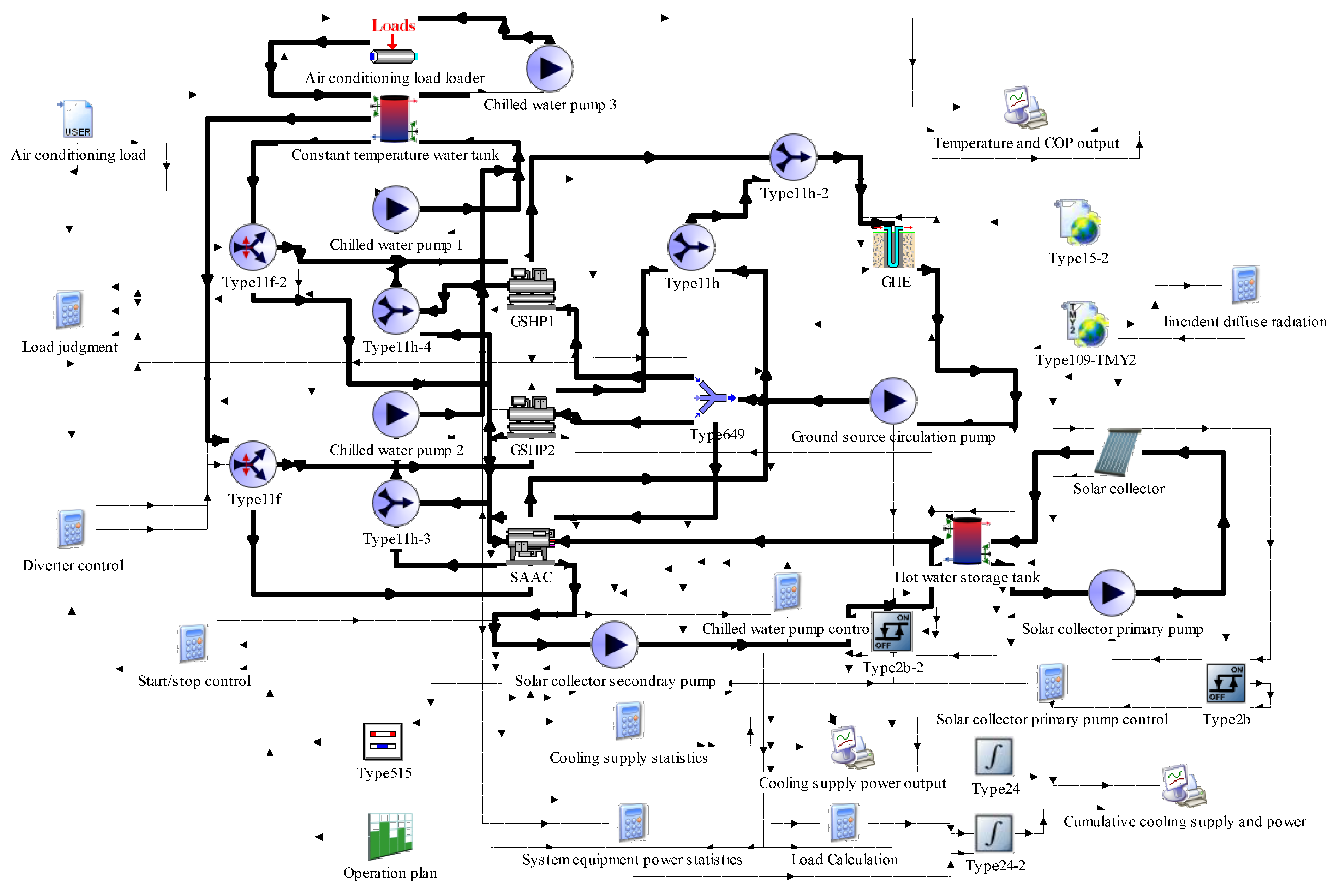
2.2. HVAC System and the Simulation Model

The HVAC system of this near-zero-energy building used a composite system of renewable and conventional energy systems. In the summer, a solar-assisted air conditioning system (SAACS) consisting of a solar collection system (SCS) and an absorption refrigeration system was used together with a ground source heat pump system (GSHPS) for joint cooling. The coefficient of performance (COP) of the absorption refrigeration unit was 0.7 and the cooling capacity was 35.5 kW. In winter, hot water generated by a SCS was used for direct heating combined with a solar-assisted ground source heat pump heating system for joint heating. Under different operating conditions, the systems operated independently and served as a backup for one another. The solar collector provided hot water to the absorption refrigeration unit. When the solar water supply temperature was higher than 75 °C, the absorption refrigeration unit could be started.

In summer, the chilled water of the low-temperature ground source heat pump (GSHP 1) handled the fresh air load and part of the cooling load of the fan coil units in the building. The chilled water of the high-temperature ground source heat pump unit (GSHP 2) handled the cooling load of the radiant air-conditioning indoor terminals in the building. The solar water tank volume and installed capacity of the heat pump were planned to adopt the optimization results, in which the heat loss of the water tank was 0.5 W/(m²·K). A total of 150 vacuum glass tube collectors were arranged on the roof to provide the heat required by the system. Eighty ground heat exchangers (GHEs) were installed in an open space on both sides of the building to provide the heat and cooling required by the building. Based on the above design conditions of the building HVAC system, the three-system operation combinations listed in

Table 3. System operation strategies.

Systems	Winter	Summer
Case 1	GSHPS	GSHPS
Case 2	GSHPS + SCS	GSHPS
Case 3	GSHPS + SCS	GSHPS + SAACS

could be obtained.

According to Table 2, there were two types of heating operation strategies in the winter: 1. When solar radiation was sufficient, the solar thermal collection system was preferred for direct heating, and the ground source heat pump system was the backup heating system. 2. Single-ground source heat-pump system for heating. There were two types of cooling operation strategies in the summer: 1. Priority was given to operating the ground source heat pump and absorption refrigeration unit, and the second ground source heat pump unit was turned on when the cooling demand could not be met. 2. Single-ground source heat-pump system for cooling. TRNSYS [21,22] was used to build system simulation models under heating and cooling conditions, as shown in Figure 2 and Figure 3, respectively. The special feature of TRNSYS is its modular analysis method. TRNSYS can call modules that implement specific functions. Under given input conditions, these module programs can simulate a specific heat transfer phenomenon and summarize the data to conduct instantaneous simulation analysis of the entire system. In Figure 2 and Figure 3, the components connected by solid lines are the equipment of the HVAC system, and the components connected by dotted lines are the programs used to control, calculate, input, and output data.

The model used for the GSHP unit was the ASHRAE chiller model. This mathematical model considers the influence of the unit load rate, cooling water temperature, and chilled-water temperature on the operating energy efficiency. The expression for the mathematical model is given in Equation (1) [21]:

$$P=a_0+a_1\left(t_{ci}-t_{eo}\right)+a_2{\left(t_{ci}-t_{eo}\right)}^2+a_3{Q}_c+a_4{Q}_c^2+a_5\left(t_{ci}-t_{eo}\right)Q_c$$

(1)

where P represents the power of the ground source heat pump unit (kW), $Q_c$ represents the load of the ground source heat pump unit (kW), $t_{ci}$ represents the inlet temperature of the cooling water of the unit (°C), and $t_{eo}$ represents the outlet temperature of the chilled water of the unit (°C).

The mathematical model of the solar water tank considered the internal stratification and heat transfer heat losses of the tank. The heat-balance equation for each layer of the water tank is given by Equation (2) [21]:

$$M_i{C}_P\frac{∆T_i}{∆t}=m_{\left(i-1\right)in}{C}_P\left(T_{i-1}-T_i\right)+m_{\left(i+1\right)in}{C}_P\left(T_{i+1}-T_i\right)$$

(2)

where $M_i$ represents the mass of the fluid in the i-th layer of the water tank (kg), $C_P$ represents the constant pressure specific heat capacity of the fluid (kJ/kg), $T_i$ represents the temperature of the fluid in the i-th layer (°C), and $m_{\left(i-1\right)in}$ represents the mass of the fluid entering the i-th layer from the i − 1 fluid layer (kg).

The solar water tank heat loss equation is as follows [22]:

$$Q_a=\sum _{i=1}^{n}U{A}_i\left(T_i-T_a\right)$$

(3)

where $Q_a$ represents the heat loss from the water tank to the environment (W), $T_i$ represents the temperature of the i-th layer (°C), $U$ represents the heat transfer coefficient of the water tank (W/(m²·K)), $A_i$ represents the surface area of the i-th layer (m²), and $T_a$ represents the ambient temperature (°C).

The parameters of the other equipment are shown in

Table 4. Transmission and distribution equipment performance parameters.

Equipment	Power/kW	Value (m3/h)
Chilled water pump 1	1.5	9.0
Chilled water pump 2	1.5	9.0
Chilled water pump 3	2.5	15.0
Ground source circulation pump	7.5	50.0
Solar collector primary pump	1.5	7.5
Solar collector secondary pump	1.0	8.5

.

2.3. Evaluation Indicators and Analysis Methods

2.3.1. Life Cycle Costs

The design of near-zero-energy buildings requires an analysis of the economic benefits throughout the life cycle of a building. The economic cost throughout the life cycle includes the initial investment and operating costs of the equipment, and is calculated according to Equation (4) [17]:

$$LCC={TC}_1+{TC}_2$$

(4)

where LCC represents the economic cost of the entire life cycle (CNY), ${TC}_1$ represents the initial investment costs (CNY), and ${TC}_2$ represents the operating costs (CNY). The operating costs are calculated using Equation (5) [17]:

$${TC}_2=\sum _1^j{C}_e\left(E_h+E_c\right){\left(1+r\right)}^{-j}$$

(5)

where $C_e$ represents the energy price (CNY/kW·h), j is the j-th year of service life of the HVAC system, and r represents the discount rate. The net present value (NPV) method is typically used to calculate life cycle costs. The operating costs must consider the annual discount rate, which is calculated according to Equation (6):

$$r=\frac{g-i}{1+i}$$

(6)

where $g$ represents the inflation rate (%) and i represents the bank interest rate (%).

2.3.2. Carbon Emission Calculation

The carbon emissions during building operation are determined according to the different types of energy consumption and carbon emission factors of each system. The total carbon emissions per unit of building area are calculated using Equation (7) [23]:

$$C_M=\left[\sum _{i=1}^n\left(E_i\ast {EF}_i\right)-C_P\right]y/A$$

(7)

where $C_M$ represents the carbon emissions per unit building area during the building operation, kg/m²; $E_i$ represents the annual consumption of type i energy of building, kW·h/a; ${EF}_i$ represents the carbon emission factor of the type i energy; i represents the type of terminal energy consumed by the building, including electricity, gas, oil, municipal heat, etc.; $C_P$ represents the annual carbon reduction of the building green carbon sink system, kg/a; y represents the design life of the building, a; and A represents the building area, m². The annual consumption of type-i energy ($E_i$) is calculated according to Equation (8) [23]:

$$E_i=\sum _{j=1}^n\left(E_{i,j}-{ER}_{i,j}\right)$$

(8)

where $E_{i,j}$ represents the type i energy consumption of the type j system, kW·h/a; ${ER}_{i,j}$ represents the amount of type i energy provided by the renewable energy system consumed by the type j system, kW·h/a; and j represents the type of building energy system, including heating, air conditioning, lighting, living systems, etc.

2.3.3. Multi-Objective Optimization

A multi-objective optimization function is established to optimize the life cycle costs and carbon emission levels during operation [24]:

$$\epsilon =min\left[\left(1-\omega \right)\times \frac{L_{op}}{L_{base}}+\omega \times \frac{C_{op}}{C_{base}}\right]$$

(9)

where $\epsilon$ represents the multi-objective optimization index; ω represents the carbon emission weighting factor—when ω is greater than 0.5, the optimization focuses on carbon emissions, otherwise it focuses on life cycle economic costs; $L_{op}$ represents the optimized building life cycle costs; $L_{base}$ represents the base building life cycle costs; $C_{op}$ represents the optimized building carbon emissions; and $C_{base}$ represents the base building carbon emissions.

The selection of the HVAC system of the base building was determined based on the needs of the designer and owner. On this basis, other configuration combinations were carried out and analyzed with multi-objective optimization, and an HVAC energy system combination suitable for the building’s design goals was achieved. The building analyzed in this project was a near-zero-energy building at a university. Its functions included office and scientific research, and the air-conditioning system was designed to meet the requirements of these two functions. The base energy system used in the design was a GSHPS. Other renewable energy systems were used to assist building heating and cooling and then compared with the base system to obtain the optimal configuration.

3. Design Parameter Optimization

The Taguchi method proposed by Genichi Taguchi [25] was used to optimize the design parameters of the GSHPS + SCS system.

3.1. Research Methodology

The Taguchi method uses the signal-to-noise ratio (SNR) to reduce the impact of uncontrollable factors on the experimental dependent variables and selects the optimal parameter combination with a smaller number of experiments. This study adopted larger-the-better characteristics; that is, the larger the characteristic index, the better. The SNR with larger-the-better characteristics was calculated according to Equation (10) [25]:

$$\frac{S}{N}=-10\times lg\left(\frac{1}{N}\sum _{i-1}^N\frac{1}{{\left(f/Q\right)}^2}\right)$$

(10)

where S/N (noise factor/error) represents the signal-to-noise ratio; f/Q represents the experimental dependent variable of this study; f represents the solar energy guarantee rate, ranging from 0 to 100%; Q represents the operating energy consumption, kW·h; and N represents the number of repetitions of the experiment, taking a value of 25.

The specific steps of the Taguchi method are: 1. The mean SNR values for each factor at the different levels are calculated. 2. The maximum SNR mean value at each level is selected by comparing each factor and then combining them to determine the optimal level combination when the experimental dependent variable is the largest. The experimental analysis methods include range and variance analysis. The range analysis method first calculates the range that represents the variation in the factor under study within the value range. The average of the experimental indicators of the i-th factor at the j level is then calculated. The optimization level and optimal combination of the i-th factor can be determined using the average value. The larger the range, the greater the impact of this factor on the indicator. The range analysis method can determine the impact of factors on indicators; thus, the primary and secondary orders of factors can be derived. However, it cannot identify whether data fluctuations are caused by experimental conditions or errors. On the other hand, the variance analysis method effectively distinguishes the causes of data fluctuations and divides them into two parts: changes caused by factors and errors. The variance analysis method includes steps such as calculating the sum of the squares of the deviations and degrees of freedom, and establishing an analysis of variance table for testing. The variance analysis method calculates the specific impact of each factor on the experimental indicators, that is, the factor contribution rate (PC). PC was calculated according to Equation (11) [26]:

$$PC=\frac{{SS}_F-\left(DF\ast V_{Er}\right)}{{SS}_T}\times 100\%$$

(11)

where ${SS}_T$ represents the sum of the squares of the total deviation, ${SS}_F$ represents the square of the deviation of each factor, $V_{Er}$ represents the sum of the squares of the errors, and DF represents the degrees of freedom of the factors.

The operating performance of GSHPS + SCS is closely related to parameters such as solar collector installation inclination angle, solar collector area, constant-temperature water tank volume, and heat pump capacity [27,28]. When the solar collector has a high heat collection efficiency, the solar heat collection area is the key factor that determines the solar energy guarantee rate, and the volume of the hot water storage tank has a significant impact on the heat collection efficiency. Therefore, four influencing factors were selected for the study: solar heat collection area/hot water storage tank volume (A/V), recorded as Factor A; solar collector installation inclination angle (S_T), recorded as Factor B; capacity of the heat pump unit (Q_hp), recorded as Factor C; and volume of the constant-temperature water tank (V), recorded as Factor D.

First, it was necessary to determine the level and level values of the four influencing factors. A/V was selected from the ratios of 250 m²/10 m³, 300 m²/15 m³, 250 m²/15 m³, 200 m²/15 m³, and 250 m²/20 m³. S_T, Q_hp, and V were divided into five levels at equal intervals. The specific influencing factor levels are listed in

Table 5. Impact factor level table.

Impact Factor	Factor Level
	1	2	3	4	5
Solar heat collection area/Hot water storage tank volume (A/V)/m−1	12.5	13.3	16.7	20	25
Installation angle of solar collector/°	25	30	35	40	45
Constant temperature water tank volume/m3	30	35	40	45	50
Heat pump unit capacity/kW	100	120	140	160	180

.

The simulation was performed, and f/Q was calculated using TRNSYS based on 25 groups of experimental plans in the orthogonal table. Minitab was used to generate an L₂₅ (5^4) orthogonal table for the five levels of the four factors, and the results are presented in

Table 6. Taguchi test plan and system simulation results.

No.	Factor Combination				A/V m−1	${\mathit{S}}_{\mathit{T}}$ °	V m3	Qhp kW	f/Q
1	1	1	1	1	12.5	25	25	100	1.551
2	1	2	2	2	12.5	30	30	120	1.693
3	1	3	3	3	12.5	35	35	140	1.789
4	1	4	4	4	12.5	40	40	160	1.812
5	1	5	5	5	12.5	45	45	180	1.856
6	2	1	2	3	13.3	25	30	140	1.540
7	2	2	3	4	13.3	30	35	160	1.638
8	2	3	4	5	13.3	35	40	180	1.660
9	2	4	5	1	13.3	40	45	100	1.405
10	2	5	1	2	13.3	45	25	120	1.432
11	3	1	3	5	16.7	25	35	180	1.883
12	3	2	4	1	16.7	30	40	100	1.615
13	3	3	5	2	16.7	35	45	120	1.689
14	3	4	1	3	16.7	40	25	140	1.711
15	3	5	2	4	16.7	45	30	160	1.795
16	4	1	4	2	20	25	40	120	1.839
17	4	2	5	3	20	30	45	140	1.935
18	4	3	1	4	20	35	25	160	1.929
19	4	4	2	5	20	40	30	180	2.029
20	4	5	3	1	20	45	35	100	1.784
21	5	1	5	4	25	25	45	160	1.809
22	5	2	1	5	25	30	25	180	1.825
23	5	3	2	1	25	35	30	100	1.628
24	5	4	3	2	25	40	35	120	1.716
25	5	5	4	3	25	45	40	140	1.739

.

3.2. Taguchi Experimental Data Analysis

Based on the variance analysis method, a significance test was performed to analyze the influence of each factor on f/Q. According to the test results, the contribution rate of each factor to f/Q could be calculated using Equation (5). The significance and contribution rate of the influence of each factor on f/Q are listed in

Table 7. The significance of the influence of each factor on f/Q and the contribution rate.

Factor	Degree of Freedom	Sum of Squared Deviations	Mean Square	Variance Statistics F	Significance Probability P	Contribution Rate
A	4	0.34389	0.08601	1941.31	<0.001	59.25
B	4	0.00152	0.00042	8.68	0.005	0.51
C	4	0.01438	0.00351	78.51	<0.001	3.65
D	4	0.20113	0.05032	1134.25	<0.001	36.21
Error	8	0.00034	0.00003	—	—	0.38
Sum	24	0.56079	—	—	—	—

. It can be found that the variance statistics value of Factor A reached 1941.31, followed by factors D and C, and that of Factor B was the smallest. Therefore, Factor B had better stability. The ranking of the contribution rates of each factor to f/Q was as follows: Factor A (59.25%) > Factor D (36.21%) > Factor C (3.65%) > Factor B (0.51%). The results of the significance test analysis of each factor mainly depended on the significance probability P. The P values of factors A and D were less than 0.001, indicating that factors A and D had a significant influence on f/Q; the P value of Factor B was 0.005, indicating that the influence of Factor B on f/Q was not obvious. The contribution rate of the error was the smallest (0.38%), which showed that the Taguchi method effectively reduced the contribution rate of the uncontrollable factors to f/Q.

Figure 4 shows the results of the main effect analysis of each f/Q factor using SNR. It can be found that A/V had the greatest influence on f/Q, and S_T had the smallest influence on f/Q. The SNR exhibited a monotonic increasing trend with an increase in Q_hp. The influence of each factor on f/Q was ranked from high to low as A/V > Q_hp > V > S_T.

The range analysis method was used to analyze each factor, and the mean responses of each factor are listed in

Table 8. The mean response of each factor.

Factor Level	A A/V/m−1	B ST/(°)	C V/m3	D Qhp/kW
1	1.739	1.721	1.685	1.601
2	1.531	1.742	1.735	1.672
3	1.741	1.737	1.761	1.745
4	1.905	1.731	1.732	1.801
5	1.742	1.719	1.737	1.855
Range	0.367	0.021	0.071	0.256
Sorting	1	4	3	2

. It can be seen that A/V had the greatest range value (0.367), while S_T had the smallest range value (0.021). Therefore, the fluctuation in S_T was minimal. The optimal level could be selected according to the f/Q corresponding to each factor at different levels, and the optimal combination was A4B2C3D5. That is, when A/V = 20 m⁻¹, S_T = 30°, V = 40 m³, and Q_hp = 180 kW, f/Q reached its maximum value.

4. Results and Discussion

4.1. Simulation Model Accuracy Validation

The experimental operation results of the GSHP + SCS system from December to February of the following year were compared and analyzed with the model simulation results. The results are shown in Figure 5. Figure 5a shows that the deviation between the experimental solar collector heat production and the simulation in December was 4.88%; the deviation in January was smaller, 1.58%. The deviation between the experimental total system heat production and the simulation in December was 4.31%, and the deviations in January and February were 4.15% and 2.60%, respectively. Figure 5b shows that the average deviation between the experimental solar fraction and the simulation during the comparison period was 2.87%, and the deviation in January was larger, 4.29%. The deviation of all operating effects between the simulation model and the experimental system was less than 5%, which indicated that the simulation model was sufficiently accurate.

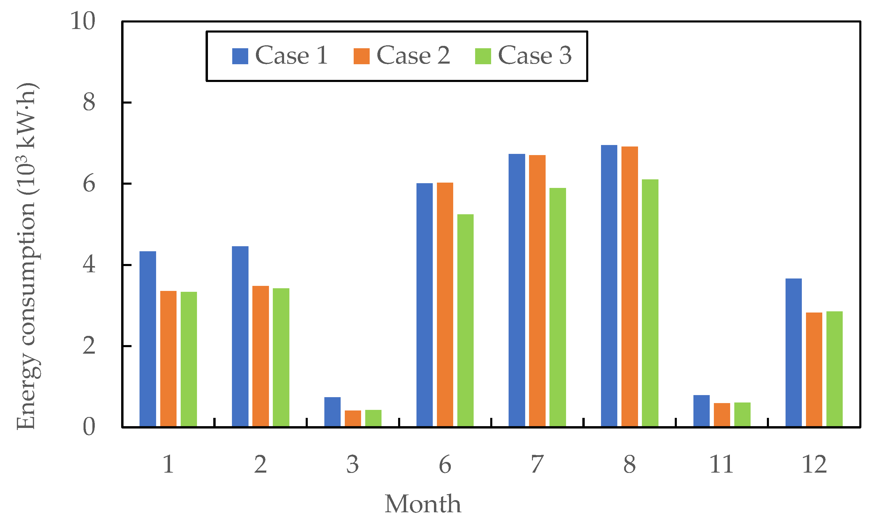
4.2. System Energy Consumption Optimization Analysis

The simulation model established by TRNSYS was used to simulate and analyze the annual energy consumption of the HVAC system. In summer, the system used the GSHPS for cooling and the SCS handled part of the domestic hot water load. In winter, the GSHPS and SCS jointly provided heating. The indoor temperature was set to 26 °C during the cooling season and 18 °C during the heating season, with temperature fluctuations of ±1 °C. During the working hours of 6:00–18:00 in the cooling and heating seasons, the simulation model determined the operating status of the HVAC system according to the input meteorological parameters and physical characteristics of the building model. Figure 6a,b shows the system operating energy consumption and solar energy guarantee rate during the heating and cooling seasons before and after the system was optimized using the Taguchi method. For the program to function properly, it is necessary to ensure that the building cooling and heating load requirements are met, and it can be observed that the solar guaranteed rate of the optimized system under this condition increased by 4.6% on average. The reduction in the installation inclination angle of the solar collector reduced the useful heat gain from the solar energy, thereby increasing the operating energy consumption of the system. Therefore, the operating energy consumption of the system decreased slightly from June to September. The annual operating energy consumption of the system was reduced by 7.32%. It should be noted that in March, which is the transitional month, the building air conditioning load was very small. Free solar heating could be achieved when the temperature of the solar hot water was higher than 45 °C and the GSHP unit was not started at this time. November is also a transitional month and its working conditions were similar to those of March. Therefore, the start-up time of the GSHP unit was shorter in these two months, and the energy consumption of the system was lower than in the other months.

The annual system energy consumption of the three system solutions in Table 2 was compared. Figure 7 shows a comparison of the total energy consumption of the three cases and their main energy-consuming equipment. Figure 8 shows a comparison of the monthly energy consumption of the three cases. Compared to Case 1, which completely adopted GSHPS for heating and cooling, the total energy consumption of Case 2 was reduced by 3121 kW ·h, accounting for 9.3%. The energy consumption of the pumps, GSHP 1 was reduced by 23.5%, and GSHP 2 was reduced by 3.6%, 23.5%, and 4.3%, respectively. The total energy consumption of Case 3 was reduced by 5677 kW·h, accounting for 17.0%, of which the energy consumption of the water pumps was reduced by 2.7%, the energy consumption of GSHP 1 was reduced by 23.6%, and the energy consumption of GSHP 2 was reduced by 25.8%. For a nearly zero-energy building in Beijing, solar thermal heating had better energy-savings benefits owing to the large heat load. Because the start-up of the absorption refrigeration unit required a high hot water temperature, the energy-savings benefits of solar-driven absorption chillers during the cooling season were lower than those of solar heating during the heating season.

4.3. Life Cycle Economic Analysis

The three cases had different initial investment and operating costs. The life cycle costs of the HVAC system under different configurations were calculated considering the initial investment cost, operating costs, and operating cost discount interest rate. Considering that the life cycle of each piece of equipment was 20 years, the investment payback period was calculated based on Case 1. The external cost of coal power was 0.38 CNY/kW·h, the electricity price was 0.8 CNY/kW·h, the inflation rate was 7.5%, and the base interest rate was 4.35% [29]. The life cycle costs and investment payback periods of each configuration are listed in

Table 9. Life cycle costs and static investment payback period.

	Cost (Thousand CNY)
	Case 1	Case 1	Case 1
GSHP unit 100 kW	196	196	196
Absorption refrigeration unit 40 kW	—	—	205
Vacuum tube solar collectors 150 sets	—	55	55
Solar collector primary pump	—	3.6	3.6
Solar collector secondary pump	—	3.6	3.6
Hot water storage tank)	—	7.5	7.5
Constant temperature water tank	12.5	12.5	12.5
Chilled water pumps	27	27	27
Ground source circulation pump	30	30	30
Well drilling costs of GSHPS	220	220	220
Initial investment	485.5	555.2	760.2
System operating costs	873.6	784.2	721.3
Life cycle costs	1356.1	1339.4	1461.5
Static payback period	—	16.1	35.5

.

It can be found that when Case 2 was adopted, the life cycle costs were the lowest, and when Case 3 was adopted, these costs were the highest. The initial investment and operating costs accounted for 36% and 64%, respectively, in Case 1; 41% and 59%, respectively, in Case 2; and 52% and 48%, respectively, in Case 3. Case 3 had the highest initial investment ratio and lowest operating costs, indicating that Case 3 had the best energy-savings effect. However, based on Case 1, the static payback period of Case 2 was 16.1 a, and that of Case 3 was 35.5 a, which could not be recycled within the life of the equipment. This was mainly because the investment cost of absorption chillers is high and the operating heat source is unsteady solar hot water; thus, the energy-savings benefits were not obvious compared with the investment costs.

4.4. Operational Carbon Emission Calculation

The energy consumed by the building during operation was electric energy, which was converted into standard coal. The conversion coefficients for each energy source and consumption are listed in

Table 10. Energy conversion factor.

Energy Type	Unit	Conversion Factor
Standard coal	kW·h/kgce	8.14
Electric energy	kW·h/ kW·h	2.6

.

The carbon emission factor of standard coal was 2.493 kg/kg, and the operational carbon emissions of the building during its entire life cycle were calculated. Figure 9 shows the life cycle carbon emissions of the building in each case. Compared to Case 1, the life cycle carbon emissions of Case 2 and Case 3 were reduced by 9.7% and 17.7%, respectively.

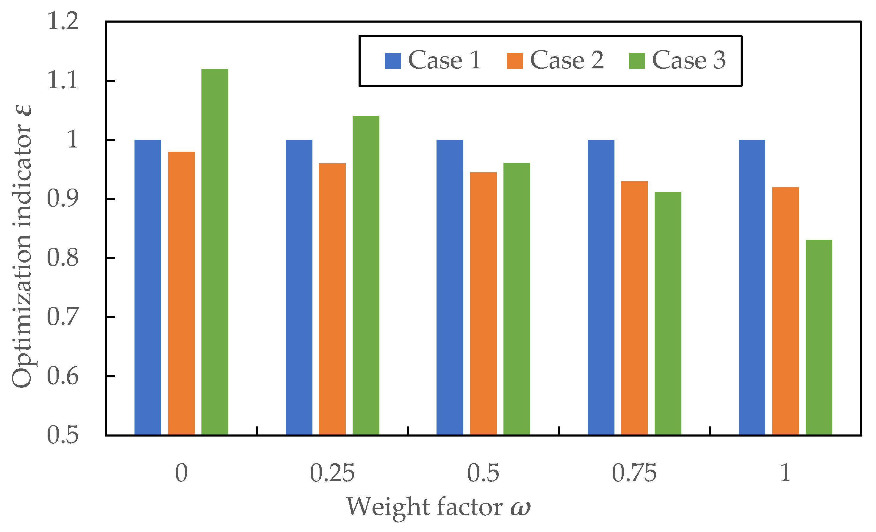
4.5. Multi-Objective Optimization Analysis

Multi-objective optimization analysis is typically used in problems in which multiple objective factors are analyzed. During the optimization process, each factor cannot simultaneously reach optimality. The non-negative weighted sum of multiple objectives must be converted into a single-objective solution optimization process. In building energy system configurations, designers usually consider factors such as the overall system economics and carbon emission benefits. These two factors were selected as optimization indicators, and their weights were set. A general energy system multi-objective optimization algorithm is established, which can modify different objective weights according to the designer’s focus. The multi-objective optimization function is given by Equation (9), in which the energy system of the case study building was analyzed from the perspectives of optimal economic efficiency, optimal environmental benefits, and comprehensive economic and environmental benefits. In Equation (9), ω is the carbon emission weighting factor. The larger the value of ω, the more the multi-objective optimization is inclined towards carbon emission benefits; the smaller the value of ω, the more economical the multi-objective optimization. The smaller the optimization index ε, the closer the case building is to the optimization goal of the designer.

Taking the near-zero energy building energy system investigated in this study as an example, a multi-objective optimization analysis was performed. The weight factor ω has values between 0 and 1, and the ε value for each case was calculated. Figure 10 shows the simulation results.

It can be found that completely using the GSHP unit for heating was not the optimal configuration from the perspective of economic or environmental benefits. When economic benefits were given priority, Case 2 was optimal, which used the GSHPS + SCS system for heating in winter and the GSHPS for cooling in summer. When environmental benefits were given priority, Case 3 was optimal, which used GSHPS + SCS for heating in winter and GSHPS + SAACS for cooling in summer.

5. Conclusions

In this study, we took a near-zero-energy building in Beijing as an example, and used TRNSYS to simulate and optimize the performance of different HVAC system configurations. Taking f/Q, the ratio of the solar energy guarantee rate to the system energy consumption, as the optimization indicator, the optimal design parameter combination was selected to optimize the system, and SNR was used to improve the accuracy of the simulation results based on the Taguchi method. We further compared and analyzed the system operating characteristics under different system configurations, established a multi-objective optimization function that optimized the life cycle costs of the HVAC system and carbon emission levels during operation, and obtained the optimal configuration under different weights. From the simulation results, it was found that:

(1)

The influence and contribution rate of the four system design factors on f/Q were ordered from largest to smallest as A/V > Q_hp > V > S_T. The optimal parameter combination for the system design was A/V = 20 m⁻¹, S_T = 30°, V = 40 m³, and Q_hp = 180 kW. Under these working conditions, the solar energy guarantee rate of the system increased by 4.6% on average, and the annual operating energy consumption was reduced by 7.32%.

(2)

For the nearly zero-energy building in Beijing, the use of GSHPS + SCS had better energy-savings benefits, but the operating costs were slightly higher. The application of absorption refrigeration can reduce system operating costs but will increase the initial investment in the system. When economic benefits are prioritized, it is optimal to use GSHPS + SCS for heating in winter and GSHPS for cooling in summer. When environmental benefits are given priority, it is optimal to use GSHPS + SCS for heating in winter and GSHPS + SAACS for cooling in summer.

References

1. Lin, Y.L.; Wang, J.J.; Yang, W.; Tian, L.; Candido, C. A Systematic Review on COVID-19 Related Research in HVAC System and Indoor Environment. Energy Built Environ. 2023, 7, 009. [Google Scholar] [CrossRef]
2. Zhang, F.; Saeed, N.; Sadeghian, P. Deep learning in fault detection and diagnosis of building HVAC systems: A systematic review with meta analysis. Energy AI 2023, 12, 100235. [Google Scholar] [CrossRef]
3. Peng, Y.Z.; Lei, Y.; Tekler, Z.D.; Antanuri, N.; Lau, S.K.; Chong, A. Hybrid system controls of natural ventilation and HVAC in mixed-mode buildings: A comprehensive review. Energy Build. 2022, 276, 112509. [Google Scholar] [CrossRef]
4. Niaki, S.O.D.; Pourfallah, M.; Ghadi, A.Z. Feasibility and investigation of residential HVAC system with combined ground source heat pump and solar thermal collectors in different climates of Iran. Int. J. Thermofluids 2023, 20, 100427. [Google Scholar] [CrossRef]
5. Ashrafi, N.; Ahmadi, R.; Zahedi, A. Technical, economical, and environmental scenario based modeling of the building equipped with ground source heat pump (GSHP) and solar system. Energy Build. 2023, 289, 113048. [Google Scholar] [CrossRef]
6. Gao, J.J.; Yan, J.J.; Xu, X.H.; Yan, T.; Huang, G.S. An optimal control method for small-scale GSHP-integrated air-conditioning system to improve indoor thermal environment control. J. Build. Eng. 2022, 59, 105140. [Google Scholar] [CrossRef]
7. Sim, M.; Suh, D.J. A heuristic solution and multi-objective optimization model for life-cycle cost analysis of solar PV/GSHP system: A case study of campus residential building in Korea. Sustain. Energy Technol. Assess. 2021, 47, 101490. [Google Scholar] [CrossRef]
8. Kaneko, C.; Yoshinaga, M. Long-term operation analysis of a ground source heat pump with an air source heat pump as an auxiliary heat source in a warm region. Energy Build. 2023, 289, 113050. [Google Scholar] [CrossRef]
9. Chen, S.Q.; Lu, M.Y.; Tan, H.W. Research on Integration Renewable Energy Systems in Office Building Based on Multi-Objective Optimization. Acta Energiae Solaris Sin. 2018, 39, 3147–3154. [Google Scholar]
10. Wakayama, H.; Sakabe, T. The outline of the heat source system that is combined with the ground source heat pump system and the aquifer thermal energy storage in the Sakata city hall. AIJ J. Technol. Des. 2016, 22, 627–630. [Google Scholar] [CrossRef]
11. Wakayama, H.; Nagano, K.; Kindaichi, S. Study of the most suitable operation of ground source heat pump system for totally electrified heating and cooling system—A practical example in a hospital. AIJ J. Technol. Des. 2009, 15, 823–826. [Google Scholar] [CrossRef]
12. Sakamoto, Y. Experimental study on the ground source heat pump system with steel pipe piles. Trans. AIJ J. Environ. Eng. 2015, 80, 785–794. [Google Scholar] [CrossRef]
13. Hai, T.; Alenizi, F.A.; Mohammed, A.H.; Singh, P.K.; Metwally, A.S.M.; Ullah, M. Optimal design modeling of an energy system for a near-zero energy restaurant with green hydrogen energy storage systems. Fuel 2023, 351, 128896. [Google Scholar] [CrossRef]
14. Cellura, M.; Guarino, F.; Longo, S.; Mistretta, M. Different energy balances for the redesign of nearly net zero energy buildings: An Italian case study. Renew. Sustain. Energy Rev. 2015, 45, 100–112. [Google Scholar] [CrossRef]
15. Shao, M.; Wang, X.; Bu, Z. Prediction of energy consumption in hotel buildings via support vector machines. Sustain. Cities Soc. 2020, 57, 102128. [Google Scholar] [CrossRef]
16. Behzadi, A.; Arabkoohsar, A. Comparative performance assessment of a novel cogeneration solar-driven building energy system integrating with various district heating designs. Energy Convers. Manag. 2020, 220, 113101. [Google Scholar] [CrossRef]
17. Wu, J.L.; Li, H.; Yu, Z.; Guo, J.W.; Lu, M.Y. Operation Analysis of a Nearly Zero Energy Building HVAC System. Build. Sci. 2020, 7, 35–41. [Google Scholar]
18. Vincenzo, B.; Eugenia, R.; Paolo, V. How the Energy Price Variability in Italy Affects the Cost of Building Heating: A Trnsys-Guided Comparison between Air-Source Heat Pumps and Gas Boilers. Building 2022, 12, 1936. [Google Scholar]
19. AlAlili, A.; Hwang, Y.; Radermacher, R.; Kubo, I. A high efficiency solar air conditioner using concentrating photovoltaic/thermal collectors. Appl. Energy 2012, 93, 138–147. [Google Scholar] [CrossRef]
20. Darko, P.; Ivan, Š.; Sandi, L.; Igor, W. Development, Calibration, and Validation of a Simulation Model for Indoor Temperature Prediction and HVAC System Fault Detection. Buildings 2023, 13, 1388. [Google Scholar]
21. Peñaloza Peña, S.A.; Jaramillo Ibarra, J.E. Potential Applicability of Earth to Air Heat Exchanger for Cooling in a Colombian Tropical Weather. Buildings 2021, 11, 219. [Google Scholar] [CrossRef]
22. Chen, C.; An, J.; Wang, C.; Duan, X.; Lu, S.; Che, H.; Qi, M.; Yan, D. Deep Reinforcement Learning-Based Joint Optimization Control of Indoor Temperature and Relative Humidity in Office Buildings. Buildings 2023, 13, 438. [Google Scholar] [CrossRef]
23. Li, X.Z.; Han, B.; Li, G.J.; Wang, K.Y.; Xu, J. Challenges of Distributed Green Energy Carbon Trading Mechanism and Carbon Data Management. J. Shanghaijiao Tong Univ. 2022, 56, 977–993. [Google Scholar]
24. Stadler, M.; Groissbck, M.; Cardoso, G. Optimal distributedenergy resources and building retrofits with the strategic DER-CA Model. Appl. Energy 2014, 132, 557–567. [Google Scholar] [CrossRef]
25. Cheng, P.; Yang, X.J.; Lan, H.; Hong, Y.Y.; Dai, Q. Design and efficiency optimization of a synchronous generator using finite element method and Taguchi method. Electr. Mach. Control 2019, 2, 023. [Google Scholar]
26. Zhang, F.B.; Yang, M.Y.; Li, Z.B. Feasibility analysis of replacing full factorial design with Taguchi method in mini-plotsoil erosion experiments. Trans. Chin. Soc. Agric. Eng. 2015, 31, 1–9. [Google Scholar]
27. Rabelo, S.N.; Paulino, T.F.; Machado, L. Economic analysis and design optimization of a direct expansionsolar assisted heat pump. Sol. Energy 2019, 188, 164–174. [Google Scholar] [CrossRef]
28. Deng, J.; Wei, Q.; Liang, M. Does heat pumps performenergy efficiently as we expected;field tests andevaluations on various kinds of heat pump systems forspace heating. Energy Build. 2019, 182, 172–186. [Google Scholar] [CrossRef]
29. Jie, D.F.; Xu, X.Y.; Liu, J.B. Research on the Impacts of Externality on Power System Optimization. J. Tech. Econ. Manag. 2021, 9, 114–119. [Google Scholar]
Figure 1. Flowchart of the optimization processes.
Buildings 13 03057 g001
Figure 2. Simulation model diagram of heating condition.
Buildings 13 03057 g002
Figure 3. Simulation model diagram of cooling condition.
Buildings 13 03057 g003
Figure 4. Main effect analysis chart of f/Q.
Buildings 13 03057 g004
Figure 5. Comparison of actual system and simulation results.
Buildings 13 03057 g005aBuildings 13 03057 g005b
Figure 6. Comparison chart before and after system optimization.
Buildings 13 03057 g006
Figure 7. Comparison of energy consumption of different equipment in each case.
Buildings 13 03057 g007
Figure 8. Monthly energy consumption comparison of the three cases.
Buildings 13 03057 g008
Figure 9. Life cycle carbon emissions of each case.
Buildings 13 03057 g009
Figure 10. Optimization indicator of each case with different weight factors.
Buildings 13 03057 g010