Experimental Study of the Dimensional and Hygrothermal Properties of Hemp Concrete under Accelerated Aging

Abstract

In this article, the functional properties of hemp concrete are studied. Hemp concrete stands to reduce the carbon impact and improve the energy consumption of houses. Hence, numerous properties are measured: mass and dimension (volume) variations are found, as is the variability in hygrothermal properties (density, thermal conductivity, heat capacity, moisture buffer value, and water vapor permeability). This entry proposes three different characterization campaigns. The first is a short introduction to the spatial variability in thermal conductivity; the second is dedicated to the study of univariate variations in the mass, volume, and hygrothermal properties of hemp concrete samples. The last one tackles the aging evolution of the properties characterized during the second campaign, in which the samples follow several aging protocols, including exposure to outdoor conditions, the application of immersion-drying cycles, and the application of freeze–thaw cycles. A set of samples is kept under control conditions to allow for comparison. As the main result, spatial variability was found in the material. This is related to the random manufacturing variability or the spatial position regarding the height of the manufactured element. A high univariate variability is found across hemp concrete samples. Moreover, the storage of samples under stable reference conditions implies very little change in the studied materials’ properties, whereas all accelerated aging protocols implied major changes of properties. In particular, we observed an evolution of the thermal conductivity of the samples kept under control conditions for 4 months, with the thermal conductivity ranging from −2.7% to +6.3% with a mean evolution of +1.22%. We observed an increase in the same property, ranging from +2.7% to +18.3%, with a mean of +9.0% for samples kept for 4 months under natural outdoor conditions, an increase ranging from +7.3% to +23.6% with a mean of +15.2% for samples that had undergone 20 cycles of immersion-drying, and an evolution of this property ranging from −5.6% to +12.3% for samples that had undergone 20 freeze–thaw cycles.

1. Introduction

There is currently a consensus in the international scientific community on the responsibility of human beings for global warming and on the need to reduce the anthropogenic environmental impact. This requires reductions in both greenhouse gas emissions and the use of fossil resources [1,2]. The house-building sector could be an action lever. Indeed, it represents a very important part of the carbon footprint and a relevant share of global energy consumption [3].

Across the literature, life cycle assessment (LCA) tools are used to assess the environmental impact of materials. LCA, applied to a building, is a calculation of the global impact of the building throughout its lifespan. Some LCAs applied to buildings have shown that the most impactful phase of a building’s life is the operational phase [4,5,6,7]. Therefore, the choice of building materials could have a significant impact on the LCA of the buildings, as it is related to the thermal regulation and heat consumption of buildings [8].

Hence, among the possibilities that have currently been proposed to reduce house-building’s impact on global warming, we can quote: improvements in the quality of the regulation of the hygrothermal conditions of both existing and future buildings—which enables reductions in the impact of the operation phase on buildings’ LCA—and the use of cleaner building materials for new constructions, which enables reductions in the impact of all other phases in buildings’ LCA.

In this context, hemp concrete fulfills the two previously cited environmental impact improvement criteria. Indeed, the LCA of hemp concrete walls showed that the overall carbon footprint of the material is excellent. This result is mainly due to the CO₂ captured by the plant during its growth and to the hemp concrete’s CO₂-capture capacity during the building’s lifespan, which can mean that hemp concrete has an overall positive impact on greenhouse gas emissions [9,10,11]. Moreover, hemp concrete shows a great ability to regulate the indoor atmosphere of buildings. Indeed, bio-based concretes have the advantage of both being very good thermal insulators and being very good humidity regulators in buildings [12,13]. These abilities make this material a very good candidate to reduce buildings’ environmental impact while maintaining pleasant living conditions for the building’s occupants.

However, hemp concrete is a relatively recent material, since its implementation only started in the 1990s. Hence, there are still some related issues. The variability of the functional properties of samples of the same formulation of hemp concrete has rarely been studied in the literature. Nguyen et al. [14] studied the impact of compaction on dimensional, mechanical, and thermal properties. They showed that a higher compaction improves mechanical properties and reduces porosity, implying an increase in both density and thermal conductivity. Niyigena et al. [15] studied the impact of the number of samples that are characterized on the mechanical properties found for hemp concrete. The present article contains a study of the univariate variation in dimensional, thermal, and hygric properties on a large batch of samples of the same formulation, which is new in the literature.

Additionally, some questions remain concerning the durability of the material depending on the environmental conditions the material faces during its lifetime. Some articles regarding the aging of hemp concrete have already been released. Some accelerated aging techniques, such as immersion–drying cycles [15,16,17,18,19], freeze–thaw cycles [20,21,22,23], and exposure to natural outdoor conditions [24,25], are found. The results can vary for the same aging type from one article to another, depending on the sample’s shape, the material formulation, or the duration of the aging. For instance, study [23], regarding the freeze–thaw technique showed no effect on the structure of materials or on the reinforcement of mechanical properties after 10 cycles, while Ismail [22] found a huge impact on these aspects and the deterioration of mechanical properties after 10 cycles of the same aging type. We can also cite existing work on the application of humidification/drying cycles [22,25,26] that corresponds to the most typical constraints that the material can face in real applications, and work focusing on accelerated carbonation [24,27], which corresponds to the typical solidification process of the material in real application cases, work focusing on simple immersion for long durations [28], and work focusing on more exotic aging processes, e.g., sulfate attack [29] or mold growth [30].

The main objectives of this paper are to complete existing works, to provide new data, and to compare new findings with the literature results to access the reproducibility of the behavior observed in the literature. The article focuses on the mass, dimensional, thermal, and hygric property evolutions according to the aging technique.

For this purpose, the thermal properties of hemp concrete samples were measured. Regarding the univariate variability, the mass, dimensions and thermal properties of 88 samples sized 4 × 4 × 16 cm³ were determined after a drying phase. The univariate variability of hygric properties on 3 to 5 cylindrical samples sliced from manufactured ø11 × 22 cm samples after a particular curing time, without any prior drying phase.

This article also describes tests carried out on hemp concrete samples aged according to three distinct techniques: one set of samples was exposed to outdoor conditions, and the other two sets were subjected to two types of accelerated aging protocols, i.e., freeze–thaw cycles and immersion–drying cycles. The results of these tests were compared to those found for the reference samples that had not undergone any specific aging protocol.

As the samples are aged, attention is paid to the evolution of the physical properties of hemp concrete with respect to the applicable conditions. The aging processes applied to the samples are deliberately fast-acting in order to observe marked changes in properties within a relatively short period of time. The objective behind applying these accelerated protocols is to determine and highlight the causes leading to the observed evolution in properties and draw conclusions regarding hemp concrete aging modes.

Moreover, no study could be found in the literature on the spatial variability of this material. We therefore sought to remedy this shortcoming by both focusing on the position of the characterizations of samples made during the univariate and aging studies presented above and by characterizing a larger sample specifically manufactured for this study, namely a hemp concrete beam. On this particular sample, we studied the spatial variability in the material’s thermal conductivity on one side of the beam in 2D.

2. Materials and Methods

2.1. Materials

The hemp shiv used for this study was provided by the CHANVRIBAT company as a byproduct of hemp fiber manufacturing. Its properties are detailed in

Table 1. Hemp shiv and binder characteristics.

Hemp Shiv		Binder
Skeleton density	1380 kg/m3	75% hydrated lime containing 98% Ca(OH)2
Particle density	256 kg/m3	15% hydraulic binder
Particle length	2 to 25 mm	10% pozzolanic binder
Particle width	0.5 to 8 mm

[31].

The binder used to produce hemp concrete is the lime referred to as “Tradical PF70”. It has been specifically designed to produce hemp concrete. Depending on the mix design, the binder may be used for different applications, such as wall, lining, screed and roofing. Several designs have been proposed by the manufacturer in order to obtain the best final properties of hemp concrete for each targeted application [32]. The binder composition is listed in Table 1 [33].

2.1.1. Mix Proportions

The hemp concrete formulation studied herein corresponds to the “wall” application indicated on the technical binder sheet [33]. The mix design (by weight ratio) is given in

Table 2. Mix mass proportions.

Water (%)	Binder (%)	Hemp Shiv (%)
51.5	32.3	16.2

.

2.1.2. Samples Description

Three distinct types of test samples were required to perform both of the experimental characterizations. Their shape, number and dimensions, and the type of characterization applied, are summarized in

Table 3. Sample description.

Sample Shape	Number	Dimensions	Type of Characterization
Rectangular parallelepiped	88	Base: 4 × 4 cm2 Length: 16 cm	Random univariation and aging of dimensional and thermal properties: mass, volume, density, carbonation rate, thermal conductivity, thermal capacity
Cylinder	33	Diameter: 11 cm Height: 22 cm	Random univariation and aging of hygric properties: Moisture Buffer Value (MBV) and water vapor permeability
Rectangular parallelepiped beam	1	Length: 125 cm Height: 20 cm Width: 9 cm	Spatial variability in the thermal conductivity of the material: thermal conductivity and heat capacity

.

2.1.3. Initial Curing Conditions

Once the parallelepiped molds were filled and leveled with fresh hemp material, the samples were cured for 3 days under climatic conditions at 20° ± 2 °C temperature and 50 ± 10% relative humidity. Next, the samples were demolded and dried for 21 additional days under the same conditions, i.e., for a total curing time of 24 days.

In the case of the cylindrical samples, the samples were molded for 10 days. After unmolding, they were cured for 28 days under the same conditions as previous samples, i.e., for a total curing time of 38 days.

A hemp beam was manufactured by pouring and leveling a waterproofed laminated plywood framework with fresh material. After unmolding, the beam was stored in the curing room for 2 months.

2.1.4. Reaction Mechanisms

The hardening and cohesion of the material mainly occurred due to two reaction mechanisms [25]: binder hydration and carbonation. The chemical reactions of hydration are expressed in Equations (1) and (2). This phenomenon is enabled by the initial water in the mixture, which serves to hydrate the lime-based binder.

C₃S + H₂O → −CSH + 1.3Ca(OH)₂

(1)

C₂S + H₂O → −CSH + 0.3Ca(OH)₂

(2)

The chemical reaction equations of carbonation are given in Equations (3) and (4). CO₂ is present in the atmosphere of the curing room, along with portlandite (Ca(OH)₂) created by the hydration of lime (Equation (3)) and uncarbonated lime remaining in the material after hydration (Equation (4)).

Ca(OH)₂ + CO₂ → −CaCO₃ + H₂O

(3)

CSH + CO₂ → −CaCO₃ + silica gel + H₂O

(4)

2.2. Tests and Protocols

2.2.1. Study Description

Univariate Variability Study

The variability study consists of characterizing numerous samples in order to highlight the variations in the dimensional and hygrothermal properties of samples after their initial curing. The samples were all manufactured at the same time; hence, parameters such as mix design, manufacturing protocol and curing conditions are identical. This study will be referred to as “healthy material characterization” or “initial characterization campaign” for the dimensional and hygrothermal properties, since most samples tested in this study were subsequently used for the aging study. This variability study characterized the properties of the 88 parallelepiped samples and 5 cylindrical samples. The properties identified for each type of material are described in

Table 4. Description of the univariate variability characterization.

Sample Shape	Number	Type of Characterization
Rectangular parallelepiped	88	Mass, volume, density, carbonation rate, thermal conductivity, thermal capacity
Cylinder	5	Moisture Buffer Value (MBV), water vapor permeability

.

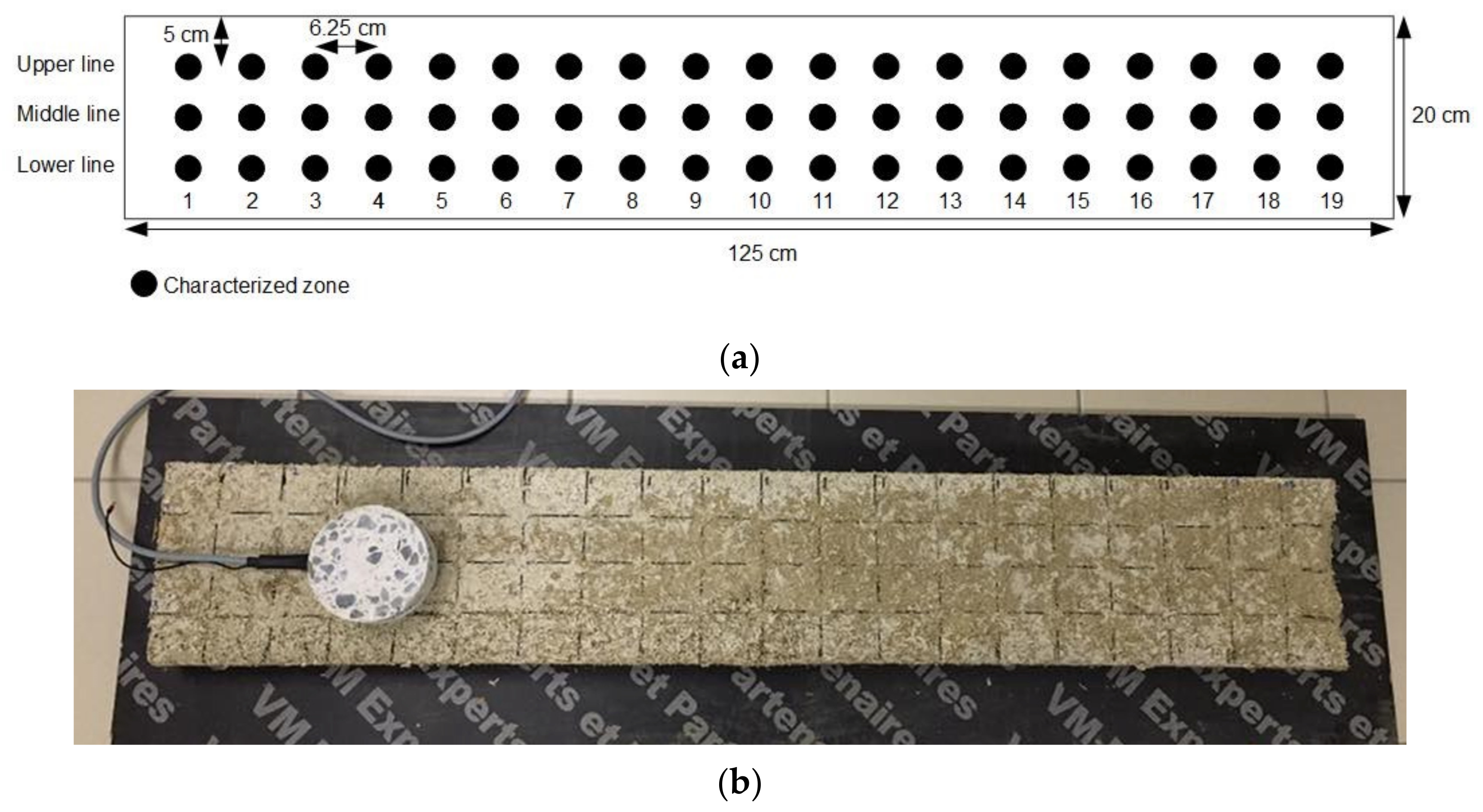
Spatial Variability Study

The spatial variability study of the material consists of locally characterizing a hemp beam in order to analyze the variation in thermal conductivity across the beam. The aim of this study was to derive the spatial distribution of thermal conductivity in a bigger sample that is more representative of a hemp wall; the results led to a greater appreciation for the material-scale study. It also seeks to determine the potential variability at a higher scale for a more accurate representation of laboratory samples. A comprehensive study will address this specific aspect. Thermal conductivity is characterized on one of the larger molded beam faces (125 × 20 cm²), while testing is performed at the intersections of a 6.25 × 5 cm² rectangular grid drawn (with a marker) on the face, as shown in Figure 1.

Aging Study

As for any material composed of organic components, the aging of hemp could constitute a significant study. The objective of this work is to derive the evolution of dimensional and hygrothermal properties, as well as drawing conclusions on the phenomena occurring in samples during aging and evaluating their impact on the material integrity. The obtained results were then compared to a set of reference materials that did not follow any specific aging protocol. The reference and aging protocols are described below.

2.2.2. Reference Conditions and Aging Protocols

Reference Conditions

The aim of introducing reference specimens was to ensure that the evolution of properties observed during aging is solely due to the aging conditions applied, rather than an intrinsic material evolution that occurs under any conditions (e.g., ettringite formation in cement-based materials). The evolution of properties in this set of samples will be compared to the evolution observed for samples undergoing aging.

The reference samples were held in the curing room after their initial characterization, like the samples used in the univariate variation study (i.e., rectangular parallelepiped samples), as well as throughout the lifetime for samples not characterized in this study, the aged specimens (i.e., cylindrical samples). The curing room conditions consisted of 20° ± 2 °C temperature, and 50 ± 10% relative humidity. The sample properties were characterized at 1 month, 2 months, 3 months and 4 months after being kept under these reference conditions; their initial curing time and ultimate initial characterization are presented in

Table 5. Aging protocol description: reference and natural outdoor specimens.

Aging Protocol	Reference	Natural Outdoor
Temperature (°C) and relative humidity (%)	T = 20° ± 2 °C, RH = 50 ± 10%	Outdoor conditions; see figure in [2]
Samples characterized after aging:	1, 2, 3 and 4 months	1, 2, 3 and 4 months

.

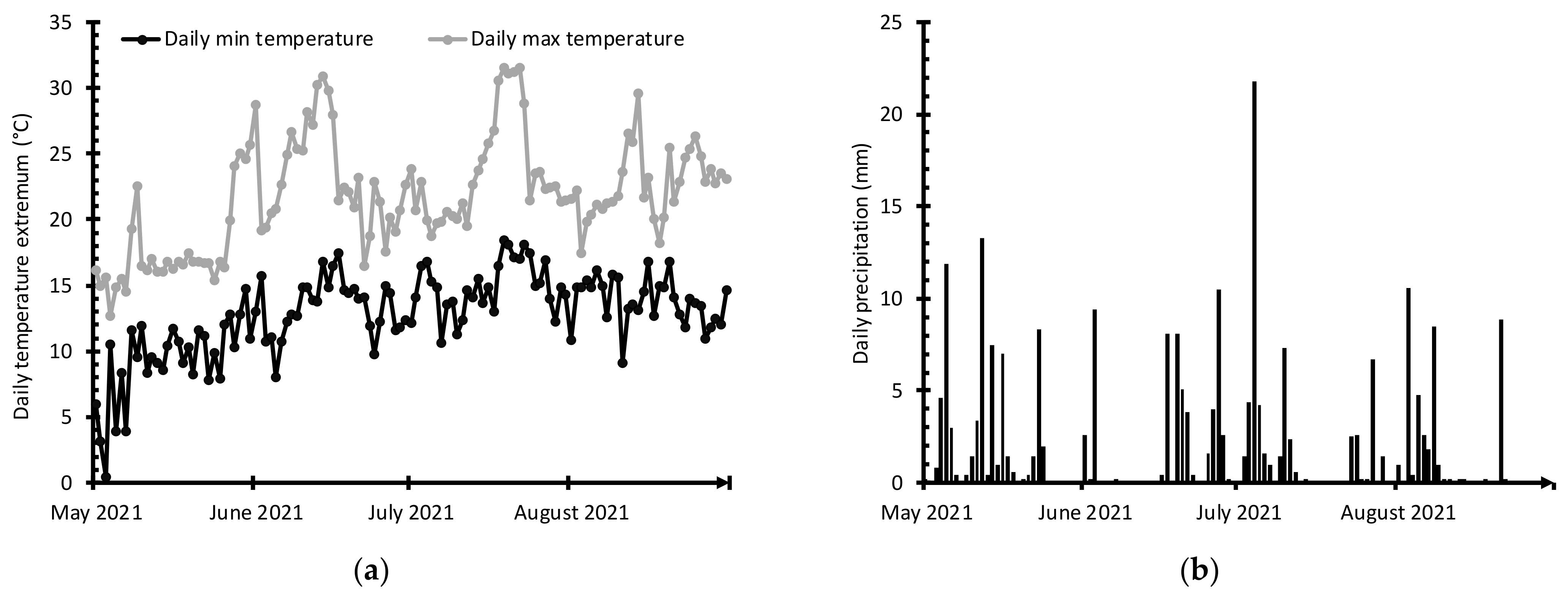
Exposure to Natural Outdoor Conditions

Exposure to natural outdoor conditions entails placing the samples outdoors. The objective of this type of aging is to study the impact of exposure to actual climatic conditions on the studied properties. The samples selected for outdoor exposure were maintained on plastic surfaces to guarantee that the evolution of properties through aging was solely due to the inherent climatic conditions. In particular, the supports ensure that samples are unaffected by any ground compound and that rainwater does not accumulate around the samples.

To effectively understand the monthly evolution of the physical properties observed after exposure to outdoor conditions, we must introduce the conditions faced by the samples during their exposure time. The two types of conditions taken into account are temperature in °C and daily precipitation in mm. For temperature, the focus is on the minimum and maximum daily temperatures, as depicted in Figure 2a. These data serve to determine if the weather was hotter or colder during specific periods, and if the amplitude of daily variations was wider or narrower. The daily precipitation levels are also shown in Figure 2b; these data are useful in indicating whether the specific periods were rainy or dry and whether the samples were confronted with especially harsh conditions during these periods. The sample properties were characterized after 1 month, 2 months, 3 months and 4 months of aging, subsequent to their initial curing time and initial characterization, if applicable (Table 5).

Immersion–Drying Cycles

Accelerated aging achieved by applying immersion–drying cycles allows for both the effect on material properties from mechanical stress due to the swelling and shrinkage generated by the repetition of cycles and the effect of potential chemical reactions between water and the material during these cycles to be studied. In the first part of the cycle, the samples are immersed in tap water at ambient temperature (20° ± 2 °C) for 48 h, while in the second part they are dried under room conditions (25° ± 2 °C, 40 ± 15% RH) for 48 h. The sample properties are characterized at 2, 4, 8, 12, 16 and 20 cycles after their initial curing time and possible initial characterization. This entire process is detailed in

Table 6. Aging protocol description: immersion–drying and freeze–thaw.

Aging Protocol	Immersion–Drying	Freeze–Thaw
Description of cycles	Phase 1: Immersion, 48 h Phase 2: Drying, 48 h Total duration: 96 h	Pre-cycle: Immersion, 48 h (once every 4 cycles) Phase 1: Freeze, 48 h Phase 2: Thaw, 48 h Total duration: 144 or 96 h
Cycle conditions	Phase 1: Underwater, T = 20° ± 2 °C Phase 2: T = 25° ± 2 °C and RH = 40 ± 15%	Pre-cycle: Underwater, T = 20° ± 2 °C Phase 1: T = −18° ± 0.5 °C Phase 2: T = 20° ± 2 °C, RH = 50 ± 10%
Samples characterized afterwards:	2, 4, 8, 12, 16 and 20 cycles	2, 4, 8, 12, 16 and 20 cycles

.

Freeze-Thaw Cycles

Accelerated aging by means of freeze–thaw cycles allows for both the effect on the material due to mechanical stress associated with the expansion of water during its liquid-to-solid state transition and the effect of the possible chemical reactions between water and the material during these cycles to be studied. To maximize the effect of freezing on the material structure, samples are pre-saturated with water by immersion phases during aging. The aim is to fill the material pores with water so that the stress caused by freezing is maximized.

Pre-saturation in water took place before the first cycle and after each of the 4 cycles. The samples were immersed in tap water at room temperature (20° ± 2 °C) for 48 h. The freeze–thaw cycles were performed in two phases. During the first phase, the samples were frozen at −18° ± 0.5 °C for 48 h, while during the second, the samples were thawed for 48 h in the initial curing room (20° ± 2 °C, 50 ± 10%). The sample properties were characterized after 2, 4, 8, 12, 16 and 20 cycles, following their initial curing time and potential subsequent initial characterization. The complete process is summarized in Table 6.

2.2.3. Testing Protocols

Conditioning Pre-Characterization

All information regarding the conditioning pre-characterization will be presented in detail below and summarized in

Table 7. Conditioning pre-characterization.

Sample Shape	Conditioning Pre-Characterization
Rectangular parallelepiped	Dried in an oven at 40 °C until the 24 h mass variation in the sample was less than 0.1% of the sample mass
Cylinder	Held at T = 20° ± 2 °C and RH = 50 ± 10% until the 24 h mass variation in the sample was less than 1% of the sample mass
Rectangular parallelepiped beam	After 2 months of curing at T = 20° ± 2 °C and RH = 50 ± 10%

.

Before any characterization steps and for all studies, the cylindrical samples were stored under curing conditions, corresponding to 20° ± 2 °C temperature and 50 ± 10% relative humidity until reaching equilibrium with the room conditions. The latter is attained once the daily relative variation in weight is less than 1% of the specimen.

Before characterization and for all studies, the rectangular parallelepiped samples were dried in an oven at 40 °C until no residual water remained. This criterion is considered to be met once the daily relative variation in mass is less than 0.1%. The 40 °C temperature threshold was chosen to allow for rapid drying while remaining low enough not to involve major changes in the material. This temperature was also selected in other studies of hemp concrete durability [23,25].

Before characterization, the beam was not subjected to any special pre-conditioning. It was directly tested at the end of its initial 2-month curing period in the curing room, which corresponded to: a temperature of T = 20° ± 2 °C, and a relative humidity of RH = 50 ± 10%.

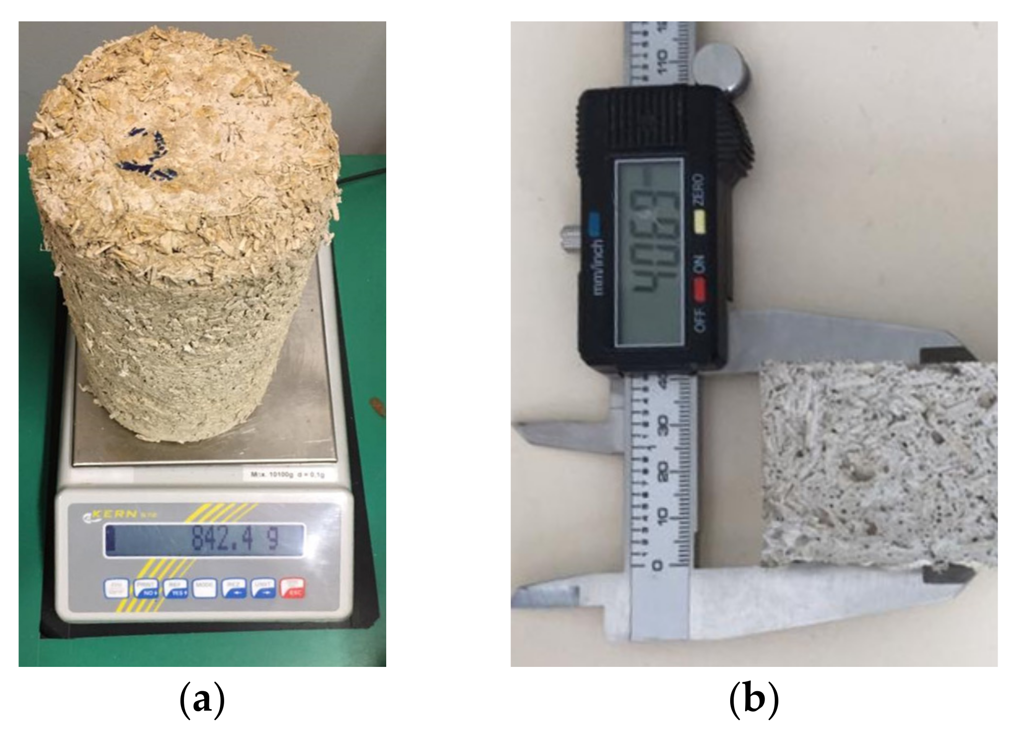
Mass, Dimension and Density

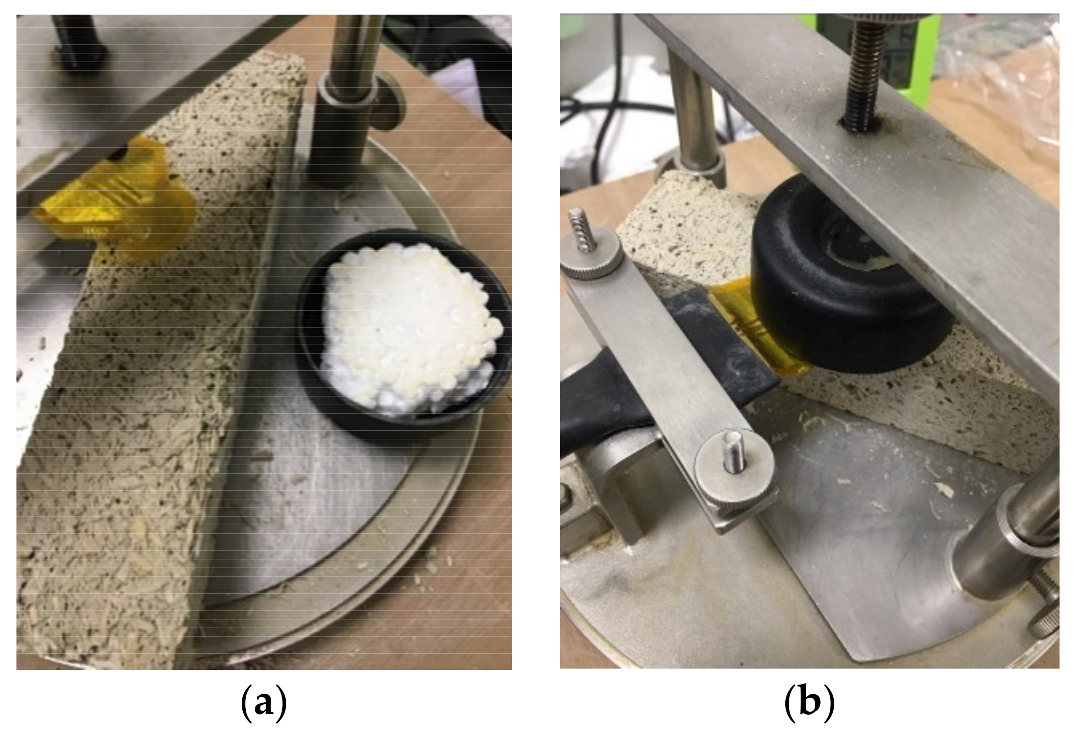
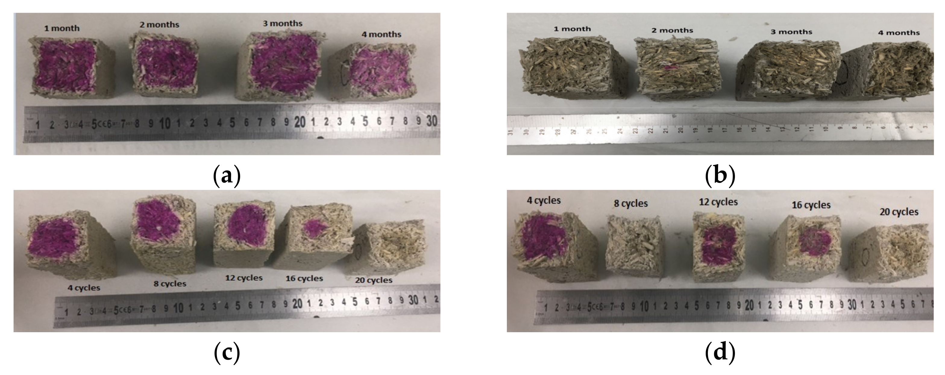
Mass was measured using scales with a 0.01 g accuracy for the rectangular parallelepiped samples and 0.1 g accuracy for the cylindrical and beam samples (Figure 3a).

For the initial characterization campaign, all specimens were weighed at the end of the curing period. Next, the rectangular parallelepipeds were subjected to the drying phase of their conditioning pre-characterization in an oven.

The samples undergoing freeze–thaw cycles were weighed after each water saturation and at the end of each cycle (i.e., after thawing). The samples undergoing immersion–drying cycles were weighed after each immersion and drying step. The samples held under reference conditions and those aged outdoors were only weighed at the end of their aging period, when they were subjected to the pre-characterization phase indicated above to obtain the new stabilized mass. The dimensions were measured using a 0.01 mm precision caliper for all samples of both shapes (Figure 3b). The rectangular parallelepipeds were measured in three dimensions: length, width, and height. Each dimension was measured at three points of the sample, with these points being distributed all along the dimension. The average value of these measurements was calculated in order to obtain better dimensional measurements. The cylindrical samples were measured in two dimensions: diameter and height. Each dimension was measured at six points of the sample, with these points being distributed all along the perimeter for the height and all around the sample for the diameter, with an angle of approx. 30° between each measurement. The average value of these measurements was calculated in order to obtain a correct approximation of the dimension. The beam dimensions were characterized just once, at the end of the curing time, using a ruler with a 1 cm accuracy for length and another ruler with a 1 mm accuracy for both width and height. Each dimension was measured six times at regular intervals to represent the total sample volume.

The sample volume can be simply estimated by considering that the specimens perfectly fit their geometric form and by using appropriate volume formula, relying on the previously obtained dimension. The density, in kg/m³, was estimated for each sample by dividing its mass in kg by its volume in m³. For the beam specimen, both the mass and volume are only known at the end of curing time; hence, the density of this sample can only be derived at that time.

Carbonation Rate

The carbonation rate of samples was measured by means of the phenolphthalein test. Phenolphthalein is a colorless acid/base indicator that turns purple when brought into contact with a material whose pH lies above 9. This case arises when the uncarbonated binder remains in the material. In contrast, carbonated lime has a pH above 9, meaning that contact with phenolphthalein will led to a transparent surface [34]. For a given surface, the carbonation rate can be determined by measuring the area of the purple surface and calculating the ratio of this area to the total tested surface area.

Furthermore, the global volume carbonation rate of parallelepiped samples was found as part of this study. To proceed, the samples were divided in two (approx. at mid-length) and the two resulting parts were subjected to the phenolphthalein test. Let us consider the result to be equal to the central surface carbonation rate of both specimens. To derive this rate, the surface dimensions were roughly 4 cm × 4 cm, corresponding to width × height. The uncarbonated area of this surface was measured with a caliper and the obtained value was then used to calculate the carbonation rate with the following formula (Equation (5)).

$$C_{rate}=\frac{S_{tot}-S_{car}}{S_{tot}}$$

(5)

where

• $C_{rate}$: carbonation rate (no units).
• $S_{tot}$: total studied surface area (m²).
• $S_{car}$: carbonated surface area (m²).

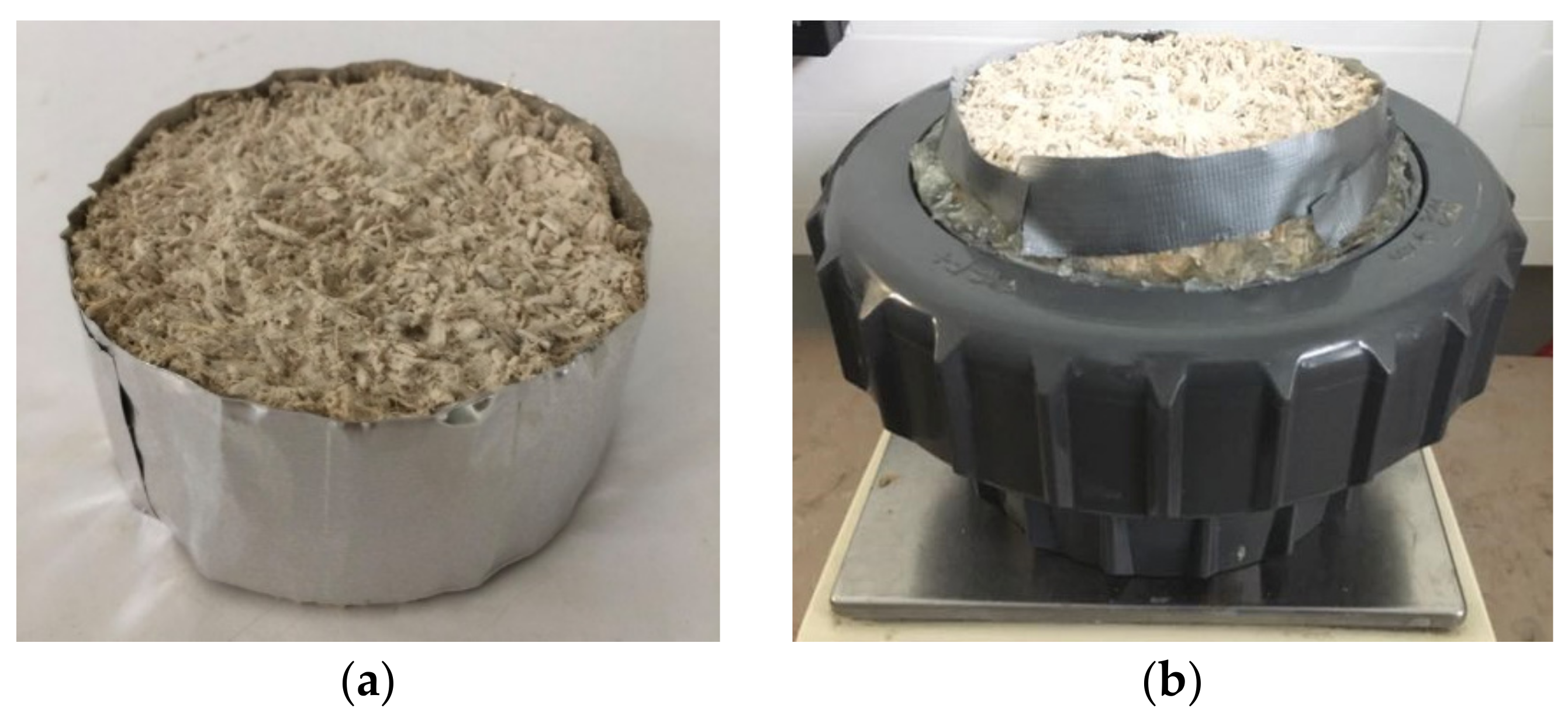
Thermal Conductivity and Heat Capacity

These measurements were conducted using the Hot Disk apparatus on both the rectangular parallelepiped samples and the beam. This protocol consists of applying heating power to a material surface using the nickel alloy resistance. The apparatus then simultaneously records the evolution in temperature at the material surface; thanks to the mathematical developments by Gustavson et al. [35], thermal properties such as thermal conductivity, thermal diffusivity and heat capacity can be determined. The experimental conditions were set as follows: heating power of 20 mW, heating duration of 20 s, a heating resistance isolated from the outside atmosphere on the upper face by polystyrene (Figure 4). It was assumed during testing that the material was isotropic. The thermal conductivity value, in W/(m.K), and specific heat capacity, in J/(kg.K), of a parallelepiped are therefore derived by taking the average of four measurements, i.e., one for each rectangular face of the specimen. For the beam, this value was obtained by a single measurement for each characterized point.

The initial result regarding heat capacity is given in MJ/(m³.K); this is then converted to the standard heat capacity unit, J/(kg.K), by dividing the result by the calculated sample density.

Moisture Buffering Value (MBV)

The Moisture Buffering Value (MBV) measurement follows the standard set forth in the NORDTEST protocol [36]. The measurement was carried out on cylindrical samples (ø11 × 22 cm) cut into slices about 5 cm thick, as recommended in the standard. This result yields the Representative Elementary Volume of the material, as found in [27,37,38]. The sample sides are laterally isolated from the exterior atmosphere by a layer of aluminum adhesive to ensure unidirectional flow inside the material (Figure 5a).

Afterwards, they were subjected to loading cycles, during which they were exposed to two distinct ambient conditions (in a climate chamber). During the first step of the cycle (8 h), the conditions were as follows: 23° ± 0.1 °C temperature, and 75 ± 2% relative humidity. During the second step (16 h), the conditions were 23° ± 0.1 °C and 33 ± 2%, respectively. The specimens’ weight increased when exposed to a high humidity (adsorption phase) and decreased when exposed to low humidity (desorption phase). No time interruption was introduced between the two consecutive cycles. Regular mass measurements were performed during each cycle. The MBV, expressed in kg/(m².%RH), could be obtained using the formula given in Equation (6).

$$MBV=\frac{ \Delta m}{S·\Delta RH}$$

(6)

where:

• $MBV$: moisture buffer value of the sample (kg/m².%RH).
• $\Delta m$: variation in sample mass over a complete cycle step (kg).
• $S$: sample surface area exposed to the atmosphere (m²).
• $\Delta RH$: variation in the air’s relative humidity between two cycle phases (%RH⁻¹).

As specified in the NORDTEST protocol [36], the experiment is to stop when the ∥∆m∥ of three consecutive cycles does not vary by more than 5%. The MBV of a sample is therefore the average values of the adsorption and desorption phases obtained for these three cycles.

For the initial campaign, five samples originating from three different cylinders (ø11 × 22 cm) were studied in order to derive the average MBV over a minimum of three samples, as recommended in the NORDTEST protocol [36]. After aging, three samples were characterized for each evaluated aging step. In these cases, and for logistical purposes, the sample pieces stemmed from one or two aged samples.

Water Vapor Permeability

The water vapor permeability measurement is performed by following the dry cup test method described in the NF EN ISO 12572 standard [39]. More specifically, cups and a climate chamber were the main equipment used for this test. The only deviation from the standard was the specimen thickness. Measurements were carried out on cylindrical samples cut into slices of approximately 5 cm, corresponding to the Representative Elementary Volume of the material [27,37,38].

The samples served as lids of cups specially designed for this type of experiment and constituted the only permeable wall separating two atmospheres with different relative humidity values, i.e., one located inside the cup, and the other outside. The sample sides were isolated from the exterior atmosphere by a layer of aluminum adhesive to ensure unidirectional flow inside the material (see Figure 5b).

The principle behind this experiment was to measure the mass exchange of water vapor between the interior and exterior atmospheres of the cup; this parameter is correlated with their water vapor pressure delta. Water vapor will migrate from the climate chamber to the cup with the lower water vapor pressure. To achieve this step, the water vapor must pass through the entire thickness of the material separating the two atmospheres, since this constitutes the only permeable wall lying between them. The more streamlined this crossing, the higher the water vapor permeability and vice versa.

The water vapor permeability, expressed in kg/(m.s.Pa), is obtained by the following formula (Equation (7)).

$$\delta =\frac{‖\frac{\Delta m}{\Delta t}‖}{S·\Delta P_v}·d$$

(7)

where:

• $\delta$: water vapor permeability (kg/(m.s.Pa)).
• $\Delta m$: mass differential between two mass measurements (kg).
• $\Delta t$: time between two consecutive measurements (s).
• $S$: surface area of the sample (m²).
• $d$: sample thickness (m).
• $\Delta P_v$: water vapor pressure differential between the interior and exterior atmospheres, which is related to the ∆RH and ∆T between them (Pa).

In our case, we applied the dry cup method. The conditions for the exterior atmosphere were as follows: 23° ± 0.1 °C temperature, 50 ± 2% relative humidity. These conditions were controlled in a climate chamber. The conditions for the interior atmosphere were T = 23° ± 0.1 °C, RH = 0 ± 5%; they were ensured by the silica gel contained in the cup. This set of conditions created a $\Delta P_v$ of around 1400 Pa between the interior and exterior atmospheres. Mass measurements of the cup were carried out every 24 h.

As a more meaningful unit of measurement, it is common to express water vapor permeability in terms of equivalent air thickness. This thickness is obtained by the formula below (Equation (8)).

$$\mu =\frac{{\delta }_{air}}{{\delta }_{mat}}$$

(8)

where:

• $\mu$: equivalent air thickness (no unit).
• ${\delta }_{air}$: water vapor permeability of air, equal to 1.95 × 10⁻¹⁰ (kg/(m.s.Pa)) at 23 °C.
• ${\delta }_{mat}$: water vapor permeability of the material (kg/(m.s.Pa)).

The reference measurement campaign took place on three unaged specimens. During these measurements of the intact material, one sample was removed from the batch to be measured. This method enabled an average water vapor permeability to be obtained for three samples, as recommended in the standard. After aging, just two pieces of samples were characterized for each aging step under study. However, given the large number of aging parameters to be tested, the values obtained after aging were most often extracted from a single specimen cut into two pieces.

3. Results and Discussion

3.1. Spatial Variation Characterization

3.1.1. Dimensional Properties

The sample characterized in this study is the beam whose dimensional properties were characterized at a global scale and hence not the subject of a spatial variability study in this article. The dimensional properties characterized are sample mass, volume and density; these characteristics were measured as follows: 10.645 kg, 0.225 m³, and 473 kg/m³, respectively.

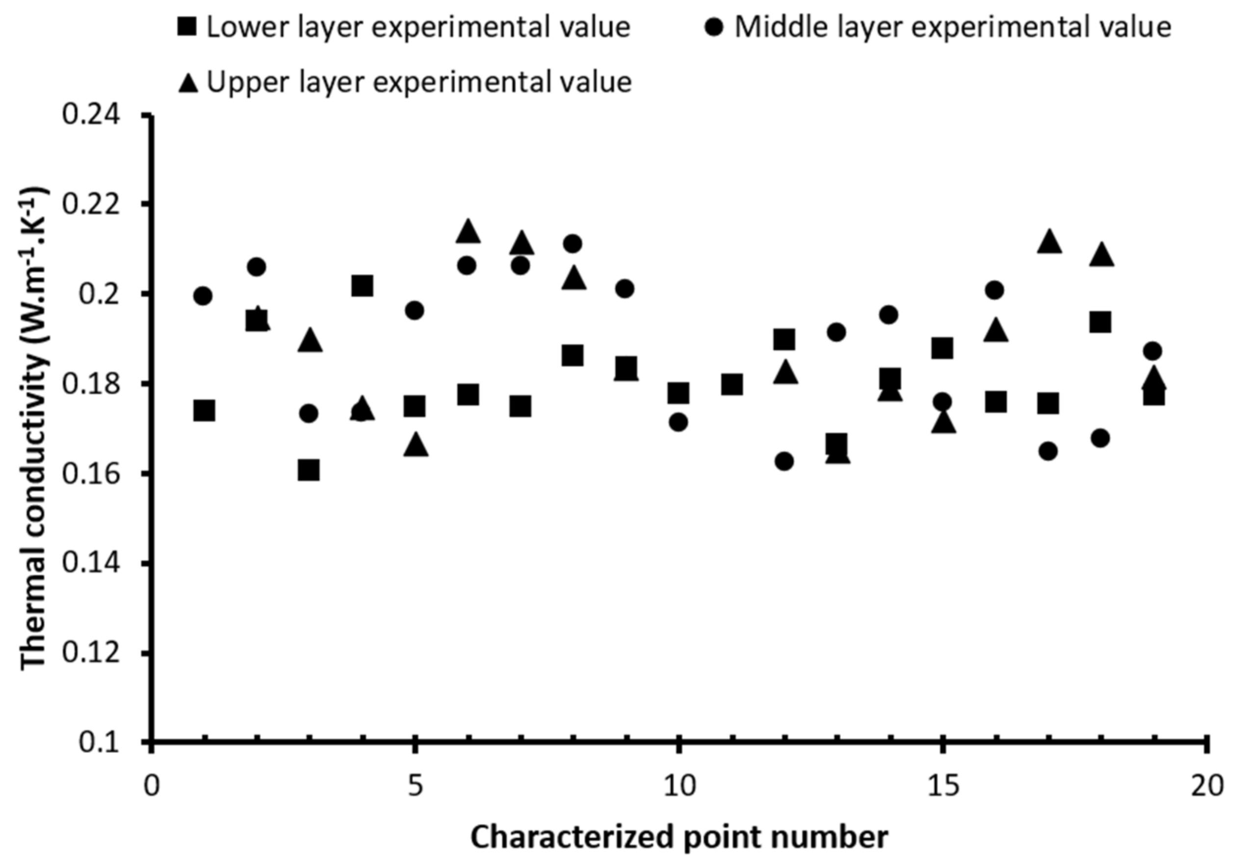
3.1.2. Thermal Conductivity Spatial Variability

The results of the beam’s layer-by-layer thermal conductivity characterization are summarized in

Table 8. Summary of spatial variability of thermal conductivity (W/m.K).

Layer	Mean	Median	Min	Max	Standard Deviation
All	0.186	0.183	0.161	0.214	0.015
Upper	0.190	0.187	0.165	0.214	0.017
Middle	0.188	0.193	0.163	0.211	0.016
Lower	0.181	0.178	0.161	0.202	0.010

. The values of thermal conductivity observed varied between 0.161 W/m.K and 0.214 W/m.K, with a median value of 0.183 W/m.K and an average of 0.186 W/m.K.

As regards the dependence of spatial variations on the characterization length, which is represented by the number of points characterized in the graph, mostly random values were observed; they did not seem to be correlated with the spatial position of the characterized point (Figure 6).

As for the correlation with characterization height, as represented by the characterized beam layer (upper, middle or lower), Table 8 shows that the properties of the upper and middle layers are relatively close. However, the lower layer shows significant differences with the other two. For this particular layer, smaller mean and median values were observed, i.e., about 5% below the other layer values. Given the smaller variations between the characterized points of this layer (as indicated by the lower standard deviation), the value for this layer is roughly 40% less than that of the others. These differences can be explained by the better tamping of this layer during manufacturing (which involves three filling and tamping phases). All tamping phases affect the lower layer (a homogeneous material), while the middle and upper layers undergo more limited tamping phases. This feature may also explain the overall lower thermal conductivity value, since it implies a decrease in the particles at the bottom of the matrix in the fresh state. These particles are hemp shiv; they are responsible for the low thermal conductivity of the entire material, as their typical thermal conductivity is below 0.06 W/m.K [40].

For a more complete view, further statistical studies would be needed to properly analyze these data and determine each variability type. However, this is not the aim of this paper.

3.2. Random Univariate Characterization

3.2.1. Dimensional Properties Random Uni-Variation

The initial dry mass of the rectangular parallelepiped samples ranged from 98.83 g to 116.15 g. Except for the extremely high values, this distribution was relatively homogeneous over this range of values, as evidenced by the quasi-linear curve that was observed. This finding was been confirmed by the proximity of the median and average values, i.e., 90.02 g and 90.28 g, respectively.

The initial dry volume of the rectangular parallelepiped samples, sorted by increasing dry volume, lies between 220.91 cm³ and 268.07 cm³. The distribution was relatively homogeneous over this range of values, as exhibited by the quasi-linear curve (Figure 7) and confirmed by the proximity of the median and average values, which equal 254.16 cm³ and 252.32 cm³, respectively. The initial dry density of the rectangular parallelepiped samples varied between 288 kg/m³ and 445 kg/m³, with a relatively homogeneous distribution over this range of values, as demonstrated by the quasi-linear curve observed and once again confirmed by the proximity of the median and average values, i.e., 365 kg/m³ and 357 kg/m³, respectively. Generally speaking, the specimens exhibited a slightly higher density than that specified by the binder manufacturer, i.e., 320 kg/m³. Nevertheless, the density values found mostly ranged from 300 to 400 kg/m³, corresponding to the expected order of magnitude. The observation of a density above the theoretical value being obtained after manufacturing has already been reported in numerous papers [12,25].

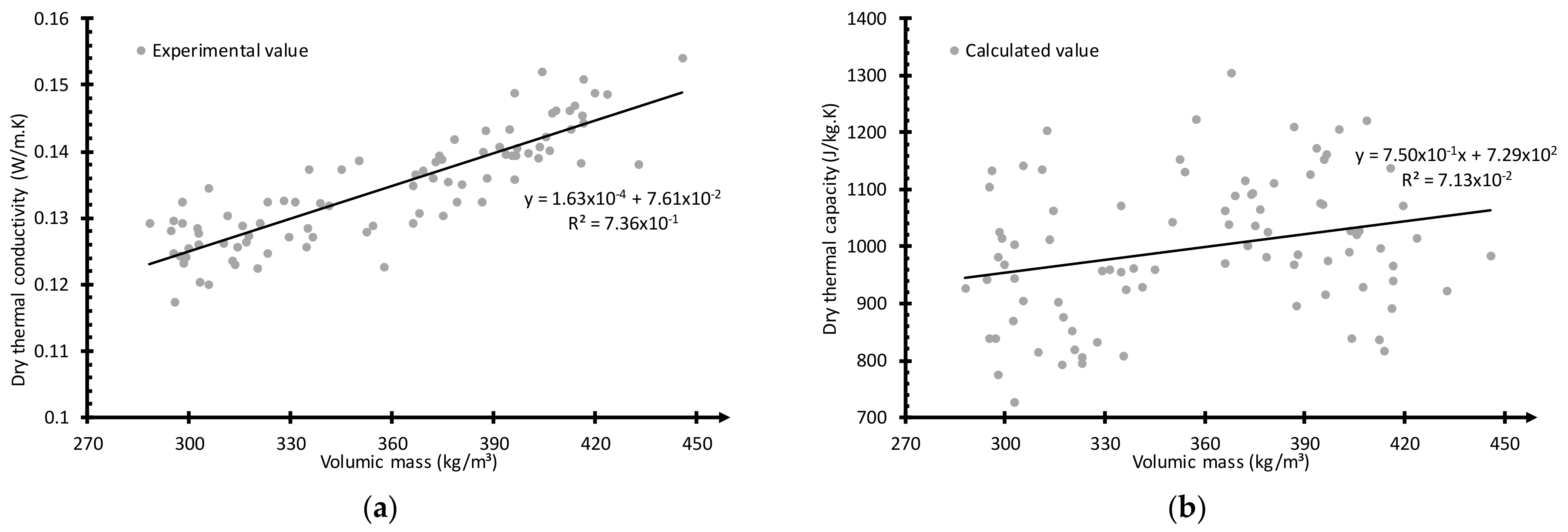
3.2.2. Thermal Conductivity Random Uni-Variation

The initial dry thermal conductivity of the rectangular parallelepiped samples is represented in Figure 7a. The thermal conductivity of the samples lies between 0.117 W/m.K and 0.154 W/m.K. The median value equals 0.134 W/m.K, while the average is also 0.134 W/m.K. The thermal conductivity value of samples tends to increase linearly with increasing density. This result corroborates theoretical expectations. These values are all higher than those specified by the manufacturer, i.e., 0.085 W/m.K. This difference may possibly be explained by the measurement method employed for this characteristic, which is local and does not reflect the global sample behavior. However, the obtained thermal conductivity values remain within the order of magnitude of those expected for hemp concrete, i.e., around 0.1 W/m.K [16,25]. Moreover, when studying the exact same material, Evrard [12] also found a higher thermal conductivity than the theoretical value.

3.2.3. Heat Capacity Random Uni-Variation

The initial dry thermal capacity of the rectangular parallelepiped samples is displayed in Figure 7b. The heat capacity of the samples lies between 764 J/kg.K and 1119 J/kg.K, with a median value of 995 J/kg.K and an average of 1000 J/kg.K. This value tends to increase slightly with an increase in density. However, the obtained values can vary quite a bit for samples within the same density range.

Unfortunately, the significant heterogeneity of the results suggests that a property was poorly characterized by the characterization method applied in our specific case. This conclusion can be correlated with the results obtained in [41], in which the authors observed a sizable deviation in the specific heat capacity measured on hemp concrete using the Hot Disk method.

Therefore, the results of this property will not be included in the aging study presented in this article.

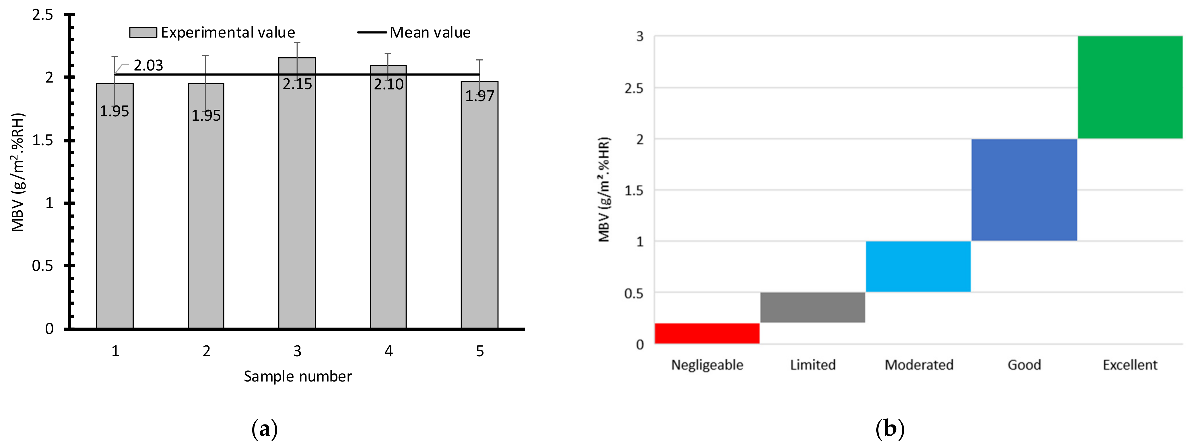
3.2.4. Moisture Buffering Value (MBV)

The initial MBV of the five cylindrical sample pieces studied herein is depicted in Figure 8a. A rather varied range of MBV values was observed, extending from 1.95 kg/m².%RH to 2.15 kg/m².%RH, with an average of 2.03 kg/m².%RH. According to the NORDTEST protocol classification, this average value qualifies hemp concrete as one of the top-tier materials for moisture buffering, as revealed by comparison with the classification given in Figure 8b. This tier corresponds to the “excellent” moisture buffer materials, i.e., a moisture buffer value above 2 kg/m².%RH. Even the sample with the lowest value still lies within the top range of the second best tier, which corresponds to “good” moisture buffer materials, i.e., those featuring a moisture buffer value between 1 and 2 kg/m².%RH. These results are in agreement with those from the bibliography [12,42]. The materials have an excellent MBV as a result of the large proportion of hemp shiv, which is indeed known for its very high water-retention capacity and fast water-retention kinetics. Studies on hemp shiv have demonstrated a typical water-retention value of around 10% of its mass in 24 h when exposed to an atmosphere with 97% humidity, thus proving that hemp concrete water retention kinetics are similar to those of hemp shiv over short durations [43].

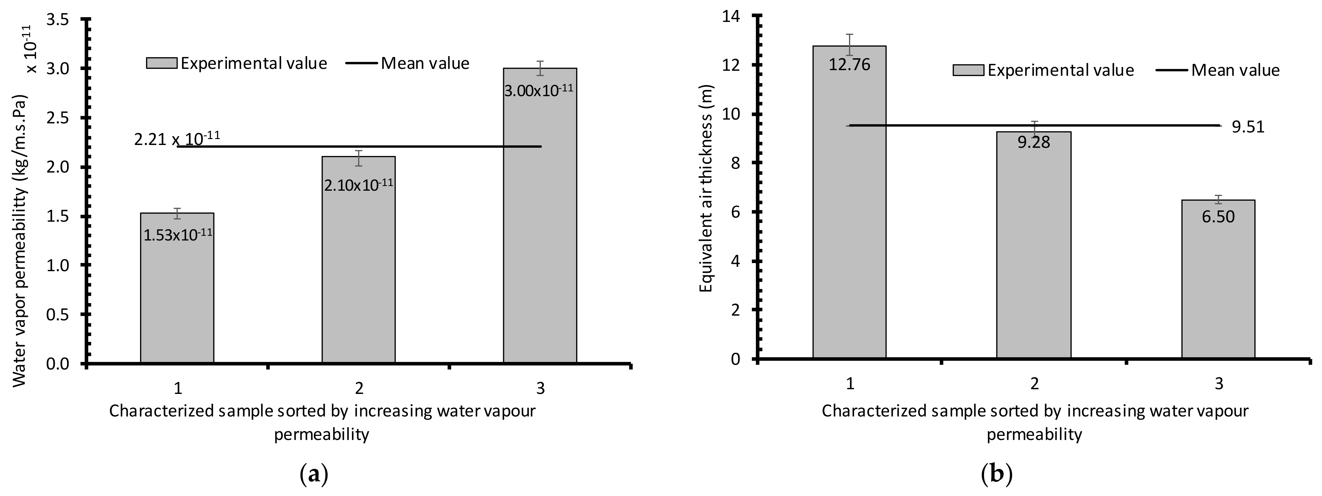
3.2.5. Water Vapor Permeability

The initial water vapor permeability of the three cylindrical samples is represented in Figure 9a. The average, minimum and maximum values are, respectively, 2.21 × 10⁻¹¹ kg/(m.s.Pa), 1.53 × 10⁻¹¹ kg/(m.s.Pa), and 3.00 × 10⁻¹¹ kg/(m.s.Pa). Overall, these results are in agreement with those of the bibliography [38,42]. However, major variations in values depending on the characterized sample were observed, with values varying by up to 100%. This observation is due to the heterogeneity of the material microstructure, as the property reveals the length of the shorter path that is required for water to cross the material thickness. The large variability obtained in terms of water vapor permeability indicates that the material microstructure varies significantly from one sample to another.

Converting these values to an equivalent air thickness yields the graph shown in Figure 9b. An equivalent air thickness value ranging from 6.50 to 12.76, with an average of 9.51, can be seen.

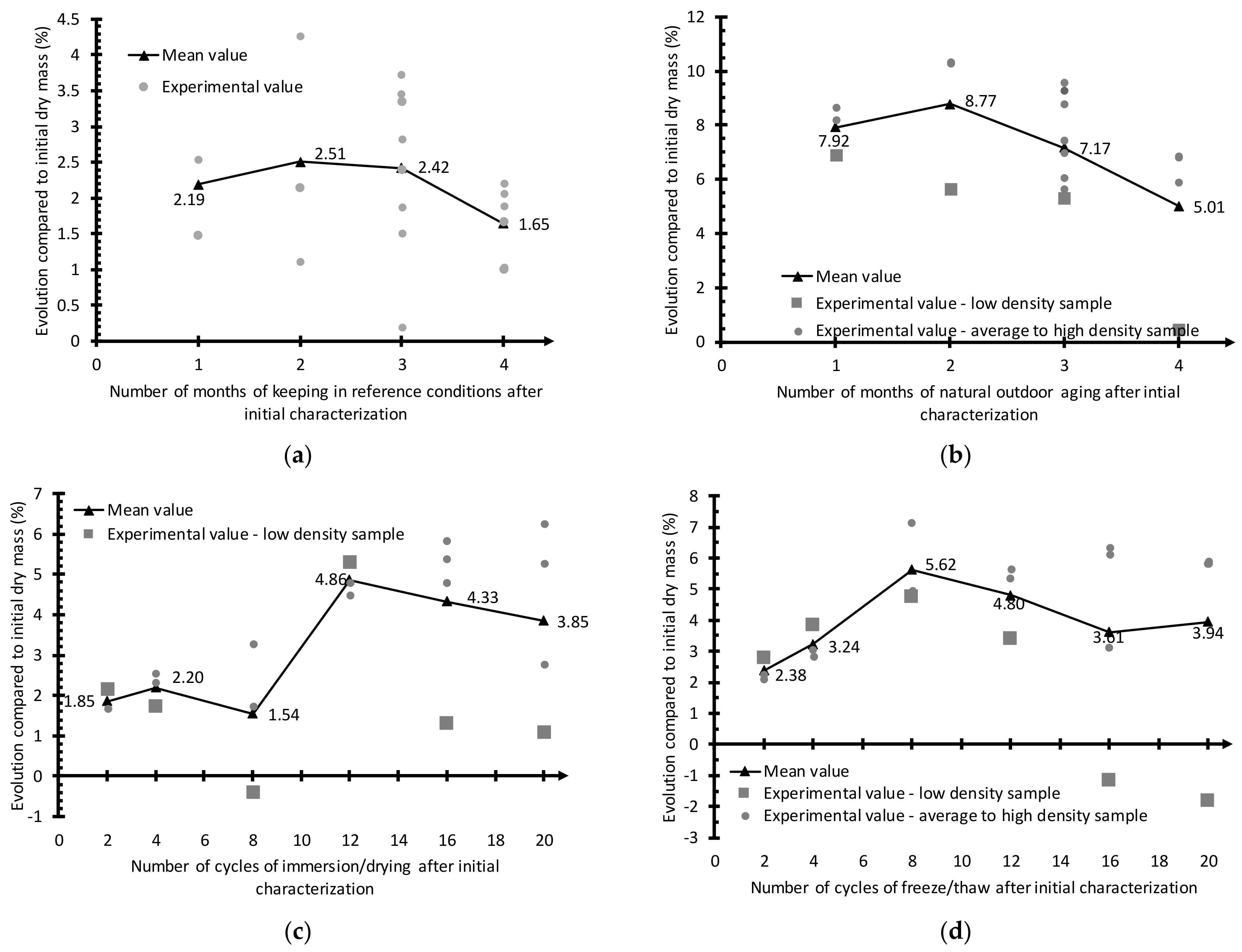
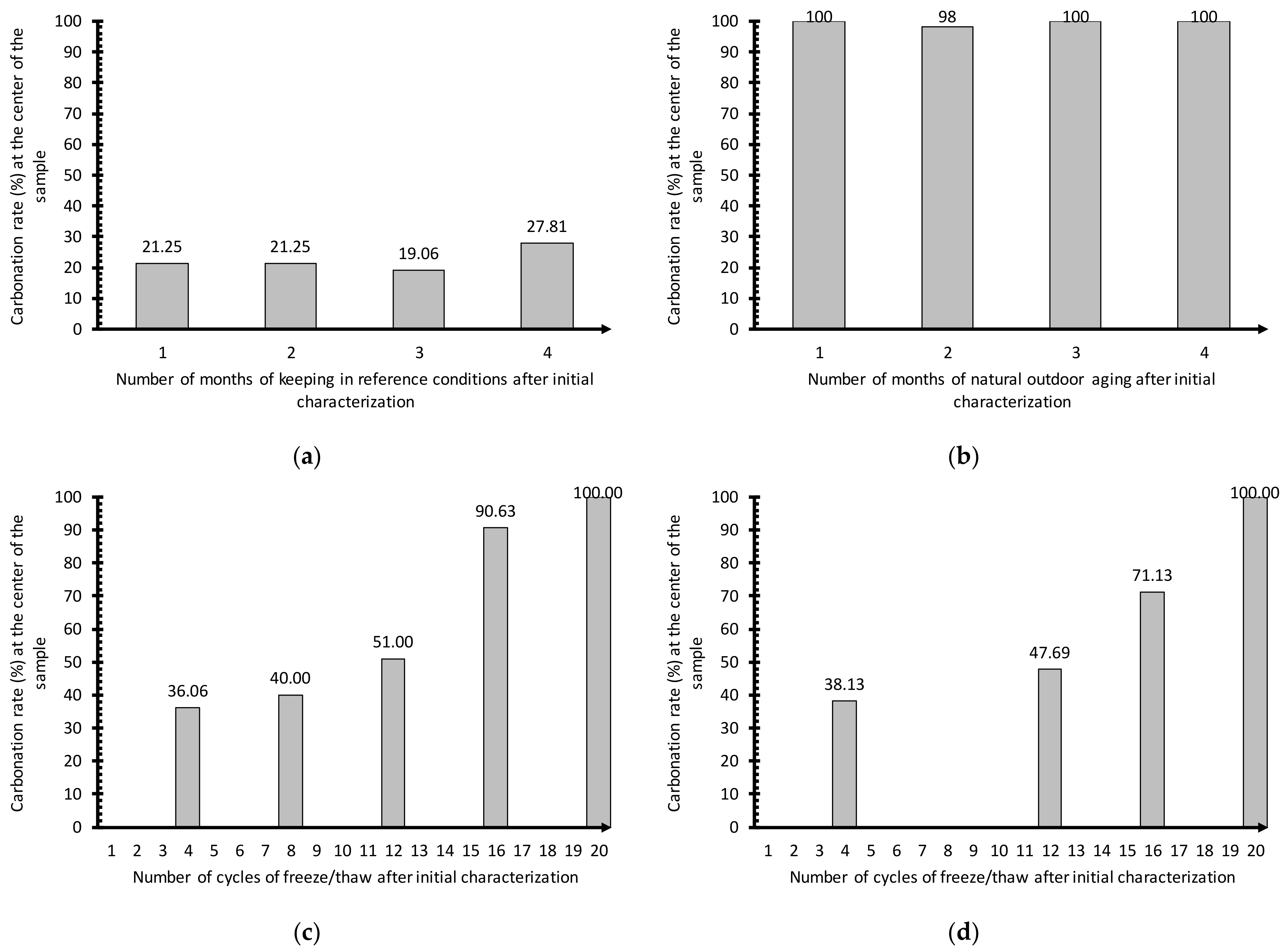
3.3. Mass and Carbonation Rate Evolution

3.3.1. Evolution under Curing Conditions

The dry mass evolution of samples held under curing conditions is shown in Figure 10a. Overall, the dry mass of samples significantly increased in comparison to the initial characterization, without any difference that can be tied to the range of initial sample densities. The increase remains constant over the months, with a mean value around 2%. More specifically, the increase was 2.19% after 1 month, 2.51% after 2 months, 1.87% after 3 months, and 1.65% after 4 months, with differences observed between the average values for different time periods and between samples in a single period, likely due to inter-sample variability and not to the action of various physicochemical phenomena. The observed increase is probably tied to a resumption of the carbonation or hydration that occurred due to contact with the air of the atmosphere in the reference conservation room. This phenomenon is enabled by the presence of CO₂ or H₂O, depending on the reaction mechanism involved, the atmosphere of the conservation room, and the presence of uncarbonated lime remaining in the material after the initial curing phase. Since the increase obtained under the reference conditions after the first month already lies around the maximum, it can be concluded that this phenomenon only occurs between the initial characterization and the first month, which is used as a reference and ceases to occur beyond that time. One possible explanation for this scenario is that carbonation or hydration occurs with re-humidification of the material after its initial complete drying and stops once equilibrium with the curing room has been restored.

This assumption is confirmed by the evolution of the carbonation rates of samples during the holding period, as presented in Figure 11a; the sample carbonation results are shown in Figure 12a. The carbonation rate remains relatively constant over the study time frame, which means that the chemical composition of the sample, as far as uncarbonated lime content is concerned, is not affected by the duration of conservation under such conditions. Considering the stability in dry mass observed over the conservation duration, this conclusion may potentially be extrapolated to the global chemical composition of samples held under such conditions.

3.3.2. Evolution under Natural Outdoor Exposure

The dry mass evolution of samples held under natural outdoor conditions is provided in Figure 10b. On the whole, the average dry mass of samples increased considerably within the first month of aging, specifically by +7.92% compared to the initial dry mass after 1 month of exposure. It then slightly increased between the first and second months, climbing to +8.77% after 2 months. This initial increase was likely due to the phenomenon of hydration and carbonation resumption. After the second month, the dry mass of the samples started decreasing, reaching +7.17% after 3 months and +5.01% after 4 months. The decreases observed during this period have different causes. The first drop was due to a small decrease in the dry mass of all samples between the second and third months of aging, while the second decrease, between the third and the fourth months, was linked to the decline in a single sample whose mass returned to its initial level before aging. This sample features the lowest density. Its initial microstructure was fragile because of its high porosity; moreover, its internal boundaries were probably destroyed by the climate, and the mass loss observed in this sample was due to a loss of material under the action of various mechanical stresses caused by multiple phenomena (rain, wind, handling). In particular, the dry mass of low-density samples, compared to their initial dry mass, rises from +6.90% after 1 month of aging to +5.66% after 2 months, 5.34% after 3 months, and finally +0.46% after 4 months of aging. For all samples, it would seem that the phenomena involving sample mass gain reached their maximum during the first two months of outdoor exposure.

The evolution in the carbonation rates for samples held under natural outdoor conditions is presented in Figure 11b, with the sample carbonation shown in Figure 12b. It can be observed that the carbonation is fully completed within the first month of aging, which means that the chemical composition of the sample is very quickly affected by such conditions, thus corroborating the conclusion drawn in the mass evolution section (i.e., indicating a maximum gain occurring very shortly after the start of aging, followed by a decrease due to a material loss as the result of a damaged structure, which is especially remarkable for the low-density sample (Figure 10b). The fact that the mass gain has not reached its maximum after 1 month of aging but instead reaches this after 2, while carbonation is complete, suggests that hydration is still occurring between the first and second months of aging and, moreover, is responsible for the mass gain observed during this period.

3.3.3. Evolution after Immersion–Drying Cycles

The dry mass evolution in samples undergoing immersion–drying cycles is shown in Figure 10c. Overall, the dry mass increases throughout the immersion–drying cycles. It starts increasing with the very first cycles, while a mean increase of +1.85% is observed after 2 cycles, +2.20% after 4 cycles, and +1.54% after 8 cycles. However, for the samples undergoing between 2 and 8 cycles, these increases are comparable to those observed for samples held under reference conditions. It may be concluded that, during this period, sample dry masses are most likely not heavily affected by any specific phenomenon tied to the application of immersion–drying cycles, but are merely undergoing a typical material evolution. It can subsequently be observed that this property continues to increase overall, probably due to the phenomenon of binder hydration and carbonation resumption. The mean value reaches a maximum at cycle 12 and then begins to decrease: a mean variation of +4.86% is recorded after 12 cycles, +4.33% after 16 cycles, and +3.85% after 20 cycles. As was the case for the dry masses of samples conserved under natural outdoor conditions, these decreases in mean value are solely due to the decrease in the mass of certain samples, while others remain relatively stable.

Those samples whose dry masses are responsible for the mean value decrease after cycle 12 are the low-density samples. Again, this can be explained by the weaker structure of these samples compared to the higher-density sample. These samples have fewer bonds and higher porosity, with these characteristics making their structure highly sensitive to the mechanical stress implied by the swelling and shrinkage phenomena that occur during wetting/drying cycles. Moreover, the high initial porosity enables water to more easily infiltrate the materials, thus resulting in higher swelling from the very beginning of the cycles. During the first few cycles, the resumption of hydration and carbonation phenomena is predominant and the structure is still intact; consequently, the masses of these samples increase. However, after a few cycles, their internal structures become damaged, and a portion of the material is lost due to the mechanical phenomena that occur during each immersion phase, which explains the mass loss during the final few cycles. The dry mass of the low-density samples, compared to their initial dry mass, moves from +5.31% after 12 cycles to +1.33% after 16 cycles and +1.08% after 20 cycles. The higher-density samples do not achieve their maximum dry mass gain after 20 cycles, meaning that their structure must be able to resist this number of cycles and potentially resist even more cycles.

The evolution of carbonation rates for the samples undergoing immersion–drying cycles is depicted in Figure 11c, while the sample carbonation is shown in Figure 12c. It can be observed that the carbonation rate increases throughout the study, which implies that the sample’s chemical composition is affected by such conditions. The increase in carbonation rate is nonlinear and, moreover, this phenomenon is slow during the first 12 cycles, which corresponds to the samples’ maximum mean mass increase; it considerably accelerates with an increase in the number of cycles. This result clearly demonstrates that carbonation occurs during aging; however, since this phenomenon continues after the maximum mass is reached for most samples, it can be concluded that this phenomenon is not responsible for most of the observed mass gain. The majority of mass gained before cycle 12 should thus be tied to the phenomenon of binder hydration resumption, while carbonation has less of an impact on this specific type of aging.

3.3.4. Evolution after Freeze–Thaw Cycles

The dry mass evolution of samples undergoing freeze–thaw cycles is shown in Figure 10d. As with the immersion–drying cycles, two distinct phenomena can be observed here, which serve to explain the overall shape of the mean value curve.

As observed in the application of immersion–drying cycle aging, the phenomena that dominate the first few cycles are the resumption of both binder hydration and carbonation, leading to a local densification of the material microstructure and resulting in a fast and continuous increase in the dry mass of samples during the first eight cycles. This effect corresponds to two immersions and eight freeze/thaw sequences; the mean values observed are +2.38% after 2 cycles, +3.24% after 4 cycles, and +5.62% after 8 cycles. At this aging time, the global mean dry mass increases to reach a maximum. For the samples with a medium-to-high initial density, a period of relative stabilization of the dry mass ensues, most likely reflecting the end of binder hydration, as described above (see the carbonation rate evolution during immersion–drying aging).

Once again, this is not the case for the low-density samples, which display a loss in the dry mass gained, with the dry mass for these samples evolving from +4.94% after 8 cycles to +3.41% after 12 cycles and continuing to decrease as the number of cycles increases: −1.15% after 16 cycles, and −1.80% after 20 cycles. This loss proves to be responsible for the decrease in the global mean dry mass. As was the case for the previous rounds of aging, this loss can be explained by the weaker structure of this sample compared to the higher-density one. Indeed, these samples have fewer bonds and a higher porosity, both characteristics that make their structure highly sensitive to the mechanical stress induced by the volume extension caused by the freezing of liquid water. Moreover, the high initial porosity enables water to more easily infiltrate the materials, thus resulting in easier water saturation from the very beginning of the cycles and higher stress induced by the freezing phase.

The evolution in carbonation rates for the samples undergoing freeze–thaw cycles is provided in Figure 11d, while the samples’ carbonation is shown in Figure 12d. It should be noted that the carbonation rate is increasing throughout the study, implying that the sample’s chemical composition is affected by such conditions; moreover, this characteristic is insufficient to fully understand the mass evolution curve for this aging pattern. Since carbonation is continuous during the study, had the phenomenon been responsible for the mass gain of samples, their mass should have increased continuously, but this was not the case. Again, this outcome proves that the phenomenon mainly responsible for the mass increase of samples is, in fact, binder hydration resumption. Since mass stops increasing after cycle 8 across all samples, it can be concluded that binder hydration is complete at this point in time.

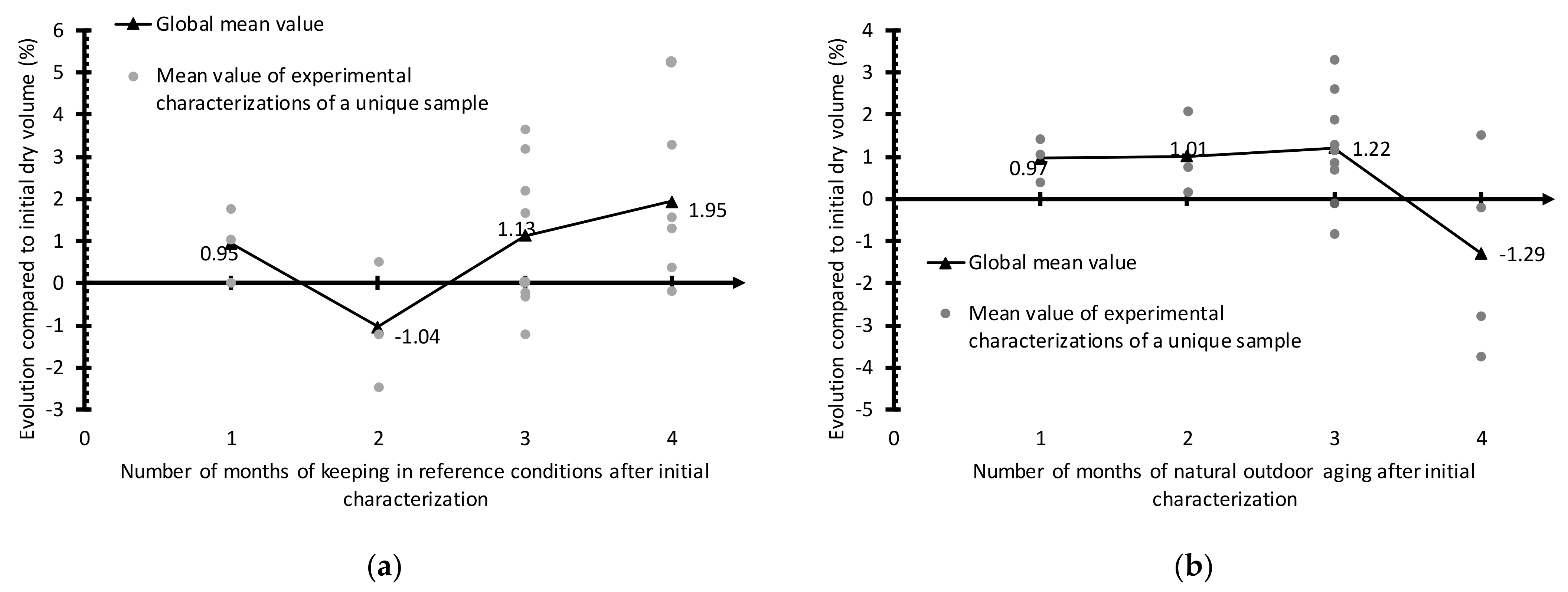
3.4. Volume Evolution

3.4.1. Evolution under Curing Conditions

The dry volume evolution of samples held under curing conditions is presented in Figure 13a; the mean dry volume overall only varied very little from the initial value. The observed variations are more likely due to the choice of different measurement points between the first characterization and the second than to any real modification of the volume during conservation. As such, it can be estimated that the maximum measurement error in dry volume is approximately 5%, which corresponds to the maximum variation recorded during conservation. This potential maximum error is high, and the typical error lies at around 2%: 10 of the 16 values obtained are in this range, which is also a high number. Volume variations in this order of magnitude for aging should thus be analyzed carefully and may be attributed to similar errors rather than actual variations in the dry volume.

3.4.2. Evolution under Natural Outdoor Exposure

The dry volume evolution of samples conserved under natural outdoor conditions is indicated in Figure 13b. The dry volume of the samples slightly evolved during the entire period of natural outdoor exposure: a mean value of +0.97% is observed after 1 month, +1.01% after 2 months, +1.22% after 3 months, and −1.29% after 4 months. It appears that the dry volume tends to increase during this aging; however, this increase is of the same order of magnitude as that observed for the reference material (±2%). Moreover, no individual variation in a single sample’s dry volume lies above the maximum difference noted for the samples held under reference conditions, i.e., ± 5%. It can therefore be considered that the sample volume changed only very slightly, or not at all, during this aging.

3.4.3. Evolution after Immersion–Drying Cycles

The dry volume evolution of samples undergoing immersion–drying cycles is shown in Figure 13c. Relatively few variations were observed in the dry volume of samples throughout the immersion–drying cycles: a mean value of +2.21% after 2 cycles, +0.03% after 4 cycles, +1.38% after 8 cycles, +1.90% after 12 cycles, +2.49% after 16 cycles, and +1.75% after 20 cycles. As was the case for natural outdoor aging, it appears that the dry volume tends to increase over the course of aging, although this increase is of the same order of magnitude as that observed for the reference material, i.e., ± 2%. No individual variation in a single dry volume sample lies above the maximum difference observed for samples held under reference conditions (±5%). It can therefore be considered that the sample volume changed very little, or not at all, during this aging.

3.4.4. Evolution after Freeze–Thaw Cycles

The dry volume evolution of samples undergoing freeze–thaw cycles is depicted in Figure 13d. A marked increase in the sample dry volume can be observed throughout the freeze–thaw cycles: compared to the initial value, the mean dry volume increased by 3.00% after 2 cycles, 1.86% after 4 cycles, 5.69% after 8 cycles, 9.27% after 12 cycles, 8.53% after 16 cycles, and by 8.91% after 20 cycles. The dry volume increase recorded during the first four cycles can be tied to measurement error since, on the whole, it remains less than 5%, which was shown to be the maximum measurement error. For the subsequent cycles, however, the increase undeniably corresponds to a physical variation in this property and not to measurement errors. This dry volume increase is due to the water expansion that occurs during the freezing phases of the cycles. During these phases, water transitions from a liquid state to a solid state, accompanied by an expansion in the global water volume that helps to destroy the boundaries constituting the internal sample structure. Thus, the initial material shape is modified by the destruction of the internal boundaries that previously ensured its stability; its volume irreversibly increases over the cycles as water widens the material pores during freezing.

The greater the number of cycles, the fewer the bonds remaining to ensure the internal cohesion of the material. Theoretically, as the number of cycles increases, the more impactful they become by causing the destruction of a larger proportion of the remaining bonds; the material’s cohesion will be significantly affected, and its volume will increase more and more sharply.

Once again, the samples most sensitive to this phenomenon are those that initially contained the fewest bonds and were the most porous, corresponding to those with the lowest initial density. These are the ones whose volume increased most significantly. The dry volume of low-density samples exposed to freeze–thaw cycles, compared to their initial dry volume, climbed from +3.01% after 8 cycles to +12.70% after 12 cycles, +16.38% after 16 cycles and +19.52% after 20 cycles. Although slower, the increases in the volume of medium-density and high-density sample are clearly observable, and the value of these increases is greater than the maximum estimated measurement error after just eight cycles: 8 of 10 samples tested in that initial density ranged showed a dry volume increase of above 5% for eight or more freeze–thaw cycles.

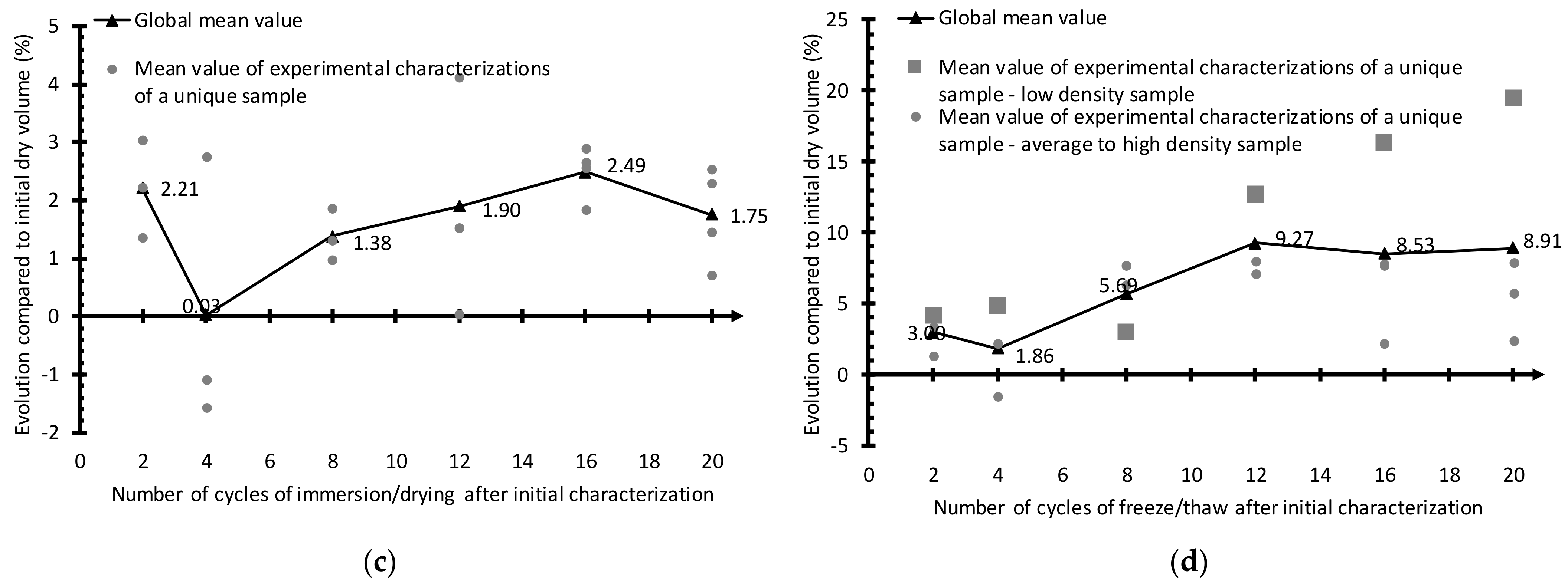
3.5. Density Evolution

3.5.1. Evolution under Curing Conditions

The change in the dry density of samples held under drying conditions is shown in Figure 14a. For this property, which depends entirely on the two preceding ones, as that it results from the division of one by the other, a very random variation can be observed: an evolution vs. the initial density of +1.23% after 1 month, +3.59% after 2 months, −0.36% after 3 months, and −0.26% after 4 months.

This random variation is mainly related to volume measurement errors, which can lead to relatively large variations in the obtained values without any real variation in volume. Consequently, this property will only be discussed for aging types that entail significant sample dry volume variations, thus ensuring that the density truly evolved. The only aging type that meets this requirement is the application of freeze–thaw cycles.

3.5.2. Evolution after Freeze–Thaw Cycles

The dry density evolution of samples undergoing freeze–thaw cycles is provided in Figure 14b. The two distinct phases observed here can explain the overall shape of the curve. Before the global increase in volume, as described above in the section dedicated to this property (occurring after the eighth freeze–thaw cycle), the sample density remains relatively stable. More specifically, the mean dry density, compared to the initial dry density, evolves as follows: −0.60% after 2 cycles, +1.41% after 4 cycles, and −0.29% after 8 cycles. This stability can be explained by the resumption of hydration, which leads to a rapid increase in the dry mass and a similar evolution in volume, either as a reflection of a physical evolution or a translation of the measurement uncertainty regarding this property.

The predominant factor in the density evolution is the significant increase in volume observed across all samples, especially the low-density ones, due to the freezing of water and the ensuing destruction of structural boundaries. This phenomenon, coupled with a halt in the evolution of dry mass linked to total binder hydration, leads to a decrease in the density of all samples. In particular, in low-density samples, the dry density keeps decreasing through the cycles, while the other sample types maintain a relatively stable dry density after cycle 12 due to a halt in their increase in volume tied to the strength of their internal structural bonding. Moreover, the average dry density of samples, compared with the initial dry density, evolves as follows: −7.03% after 12 cycles, −4.32% after 16 cycles, and −4.08% after 20 cycles. Also, the dry density of low-density samples, compared to their initial dry density, extends from −8.24% after 12 cycles to −15.06% after 16 cycles, and ultimately to −17.84% after 20 cycles.

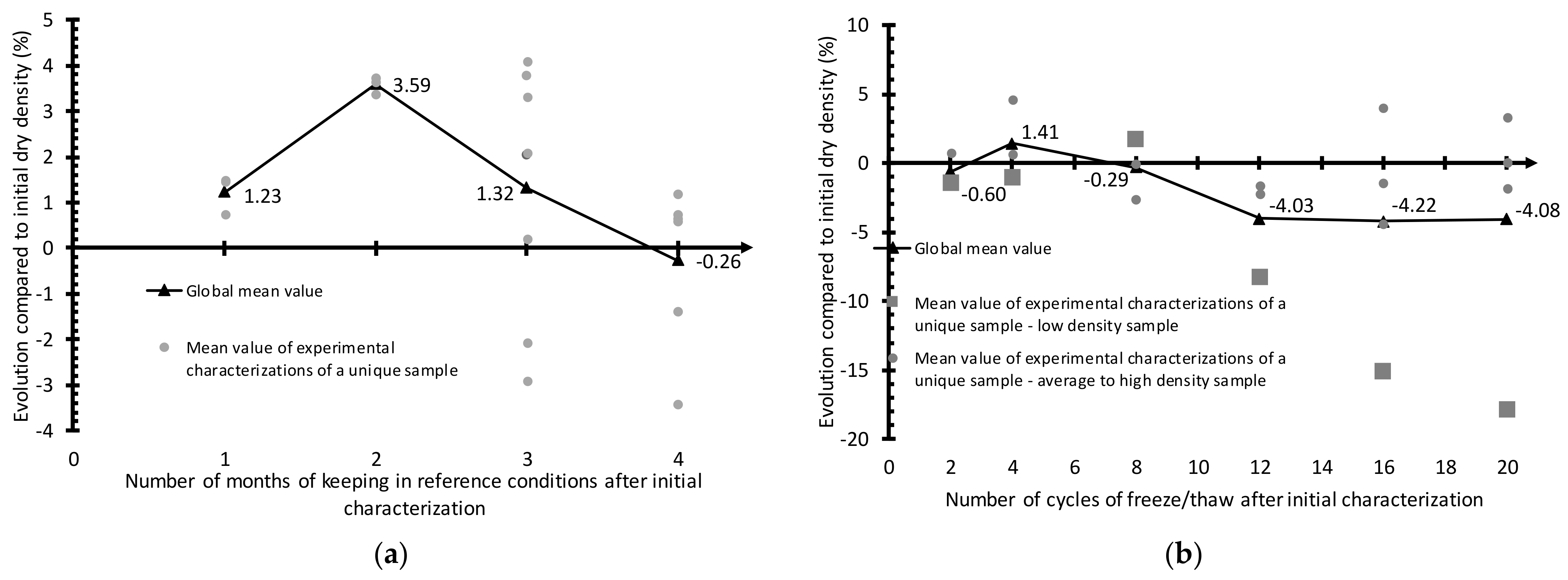
3.6. Thermal Conductivity Evolution

3.6.1. Evolution under Curing Conditions

The dry thermal conductivity evolution of samples held under curing conditions is presented in Figure 15a. It can be observed that the samples maintained under reference conditions after initial characterization display a random dry thermal conductivity evolution throughout conservation, with this evolution being characterized by a low mean variation. More specifically, the average values obtained are −0.85% after 1 month, +2.64% after 2 months, +1.02% after 3 months, and +1.22% after 4 months. The maximum variation observed for a single sample is +6.89%, while the typical thermal conductivity variation range equals ±5% over the entire conservation: 13 of 16 samples in this evolution range. The number of samples whose dry thermal conductivity increased during conservation equals the number of samples whose dry thermal conductivity decreased, i.e., eight in each case. Lastly, for this conservation sequence, no correlation can be drawn between the dry thermal conductivity evolution and the initial density of the characterized samples. The described evolution typically corresponds to a measurement error, most likely due to the choice of different measurement points between the first and second characterizations and not due to any real physical variation in the property. Under these conditions, and over these given periods, it can be concluded that the material maintains its thermal insulation capacities, which is critical since the material was specifically designed as a thermal insulator.

3.6.2. Evolution under Natural Outdoor Exposure

The dry thermal conductivity evolution of samples held under natural outdoor conditions is exhibited in Figure 15b. Overall, this property considerably increased during the first month of exposure to natural outdoor conditions, with a mean evolution of +10.89%, compared to the initial value during this month. The mean values obtained for the subsequent months of exposure remain relatively stable compared to that of the first month, i.e., +10.89% for 1 month, +10.70% for 2 months, +10.50% for 3 months, and +8.99% for 4 months. The dry thermal conductivity evolution is directly linked to the dry mass evolution: as the dry mass increases (see the section dedicated to observations), the dry conductivity increases. This behavior is logical since the mass gain is mainly due to the hydration of the remaining unhydrated lime. Moreover, conduction in hemp concrete occurs within the bonds containing this lime. When the lime is hydrated, it becomes denser and heat can be conducted through the more easily formed bonds, which are responsible, at the sample scale, for increases in both dry mass and dry thermal conductivity.

3.6.3. Evolution after Immersion–Drying Cycles

The dry thermal conductivity evolution of samples undergoing immersion–drying cycles is shown in Figure 15c. On the whole, the thermal conductivity of samples increases with the number of cycles. It increases more quickly over the first few cycles and then stops increasing for a while. The mean values recorded are +6.31% after 2 cycles, +7.43% after 4 cycles, and +7.63% after 8 cycles. This property is then seen to substantially increase compared to the initial values obtained, yet a slow decrease begins beyond this point, with mean values of +21.22% after 12 cycles, +19.48% after 16 cycles, and +15.25% after 20 cycles. The dry thermal conductivity evolution is directly linked to the dry mass evolution: as the dry mass increases, dry conductivity increases and vice versa (Figure 10c). This behavior is similar to that observed for natural outdoor conservation and features the same causes.

As is the case for dry mass, the decrease in the mean value of thermal conductivity evolution over the last few cycles is mainly due to a decrease in the thermal conductivity of certain samples, while others display a thermal conductivity that remains nearly as high as it was after 12 cycles. The type of sample, whose thermal conductivity decreases after 12 immersion–drying cycles, is the same as those whose mass decreased after the same number of cycles, namely low-density samples. The thermal conductivity, compared to the initial value of this type of sample, drops from +21.22% after 12 cycles to +19.48% after 16 cycles and +15.25% after 20 cycles. This finding is logical given that a mass loss without variation in volume leads to a loss of density; moreover, the thermal conductivity of a material increases proportionally with its density.

3.6.4. Evolution after Freeze–Thaw Cycles

The dry thermal conductivity evolution of samples undergoing freeze–thaw cycles is presented in Figure 15d. Over the short-term, i.e., during the first four cycles, the phenomenon of hydration resumption predominates in the evolution of sample thermal conductivity. Binder hydration leads to a densification of material microstructure, causing an increase in sample thermal conductivity for the same reasons as explained in the natural outdoor and immersion–drying cycle aging types. Thermal conductivity evolution rises from a mean value of +3.30% after 2 cycles to +18.43% after 4 cycles.

In the long term, as hydration tends to become complete, the destruction of internal structural bonds caused by the freezing of water predominates in the evolution of mean thermal conductivity. Firstly, for the low-density samples, a significant decrease in thermal conductivity evolution is observed, with a value declining from +12.90% after 4 cycles to +6.59% after 8 cycles, −2.98% after 12 cycles, −5.16% after 16 cycles, and ultimately to −5.64% after 20 cycles, accounting for a total decrease of 18.54% of the initial value between cycles 4 and 20. Again, this drop is due to these samples’ sensitivity to the destruction of internal bonds induced by freeze–thaw repetition, thus causing higher porosity with fewer bonds and enabling thermal energy conduction in the material.

Secondly, the thermal conductivity of the other types of samples remains relatively steady between cycles 8 and 20, i.e., between +10% and +15%, compared to the initial dry thermal conductivity, which confirms that the microstructure of these samples is relatively stable through this aging sequence, since the gain in thermal conductivity induced by binder hydration is indeed preserved.

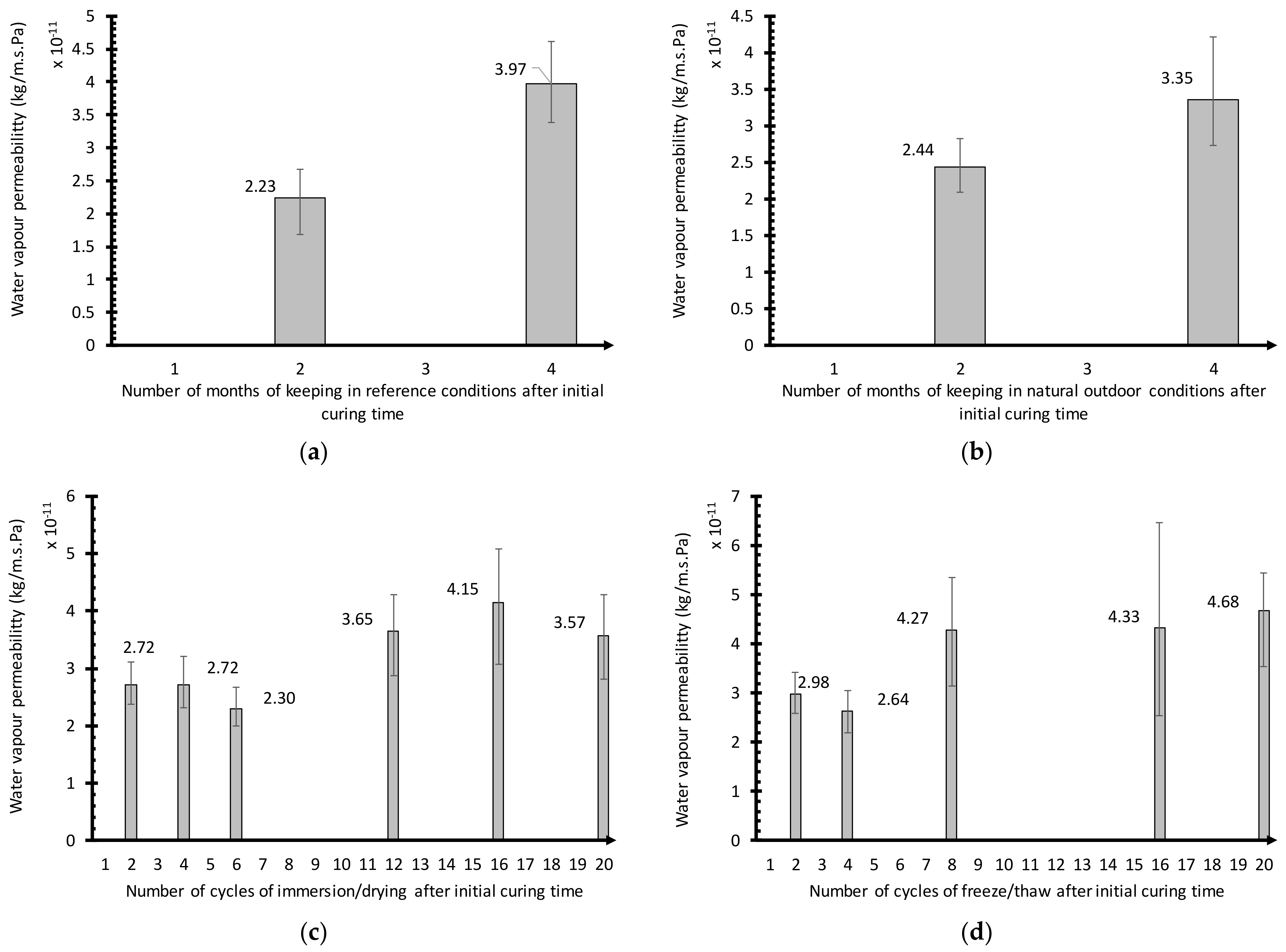
3.7. Water Vapor Permeability Evolution

3.7.1. Evolution under Curing Conditions

The water vapor permeability evolution of samples held under curing conditions is provided in Figure 16a. The mean value remains relatively constant over the first 2 months of curing. Indeed, the mean water vapor permeability obtained after the initial curing time was 2.67 × 10⁻¹¹, while that recorded after 2 months of reference conservation was 2.23 × 10⁻¹¹. However, the mean water vapor permeability increases significantly between the second and third months of conservation under such conditions, extending from 2.23 × 10⁻¹¹ after 2 months to 3.972 × 10⁻¹¹ after 3 months.

These results must be considered carefully, as the variation in water vapor permeability obtained between two samples held during the same period of time under the same conditions can be sizable. For example, during the initial campaign, performed after 1 month of curing, the water vapor permeability of a single sample was 1.81 × 10⁻¹¹, while the same property value for another sample was 3.68 × 10⁻¹¹, more than twice the value obtained for the first sample. The observed variation is likely due to differences in the microstructure of the samples used for characterization, as the material shows a highly porous and heterogeneous internal structure, which allows for different water throughflow paths. This difference is potentially significant between samples, which, in turn, can directly impact the obtained water vapor permeability.

3.7.2. Evolution under Natural Outdoor Exposure

The water vapor permeability evolution of samples held under natural outdoor conditions is provided in Figure 16b. It can be observed that the water vapor permeability after 2 months of conservation under such conditions remains relatively stable compared to the initial campaign: the mean value obtained after initial curing time was 2.67 × 10⁻¹¹, and that obtained after 2 months of natural outdoor aging was 2.44 × 10⁻¹¹. Between 2 and 4 months of conservation under natural outdoor conditions, the mean measured value increased from 2.44 × 10⁻¹¹ after 2 months to 3.35 × 10⁻¹¹ after 4 months. This increase is noteworthy, although less than that observed between 2 and 4 months of reference conservation under curing conditions, for which the mean water vapor permeability of samples rose from 2.23 × 10⁻¹¹ after 2 months to 3.972 × 10⁻¹¹ after 4 months.

3.7.3. Evolution after Immersion–Drying Cycles

The water vapor permeability evolution of samples undergoing immersion–drying cycles is presented in Figure 16c. Two distinct parts of the curve can be clearly seen.

During the first part, composed of samples that underwent between 2 and 6 immersion–drying cycles, the mean water vapor permeability is relatively stable. The mean value after 2 cycles equals 2.72 × 10⁻¹¹, vs. 2.71 × 10⁻¹¹ after 4 cycles and 2.29 × 10⁻¹¹ after 6 cycles. This range of values corresponds to that obtained during the initial characterization campaign, which yielded a mean value of 2.67 × 10⁻¹¹. The closeness of these values signifies that the aging applied at this number of cycles does not considerably affect the property.

During the second part, composed of samples that underwent at least 12 immersion–drying cycles, the water vapor permeability spikes before stabilizing. The mean obtained value climbs from 2.29 × 10⁻¹¹ after 6 cycles to 3.75 × 10⁻¹¹ after 12 cycles; it equals 4.15 × 10⁻¹¹ after 16 cycles and 3.57 × 10⁻¹¹ after 20 cycles. This value range corresponds to that obtained after the initial months for samples held under reference curing conditions, i.e., a mean value 3.972 × 10⁻¹¹ after 4 months of conservation. These close values signify that the aging applied at this number of cycles does not have a greater effect on this property than conservation under standard controlled conditions.

Overall, aging makes the material more susceptible to water vapor; this increase reflects a more porous internal structure, which exists following the destruction of the bonds during swelling and withdrawal actions linked to the immersion–drying cycles.

3.7.4. Evolution after Freeze–Thaw Cycles

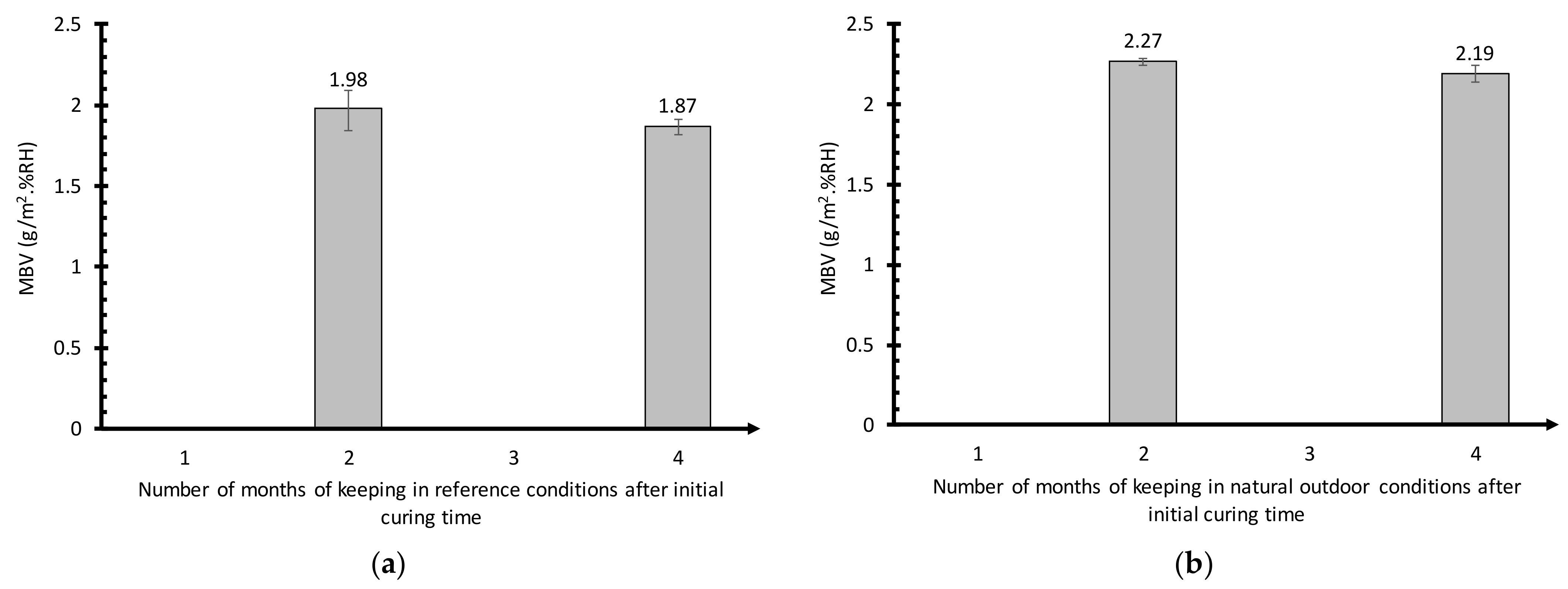
The water vapor permeability evolution of samples undergoing freeze–thaw cycles is shown in Figure 16d. Once again, two parts of the mean value curve can be clearly distinguished.

The mean value obtained after 2 cycles is 2.98 × 10⁻¹¹ and that after 4 cycles is 2.64 × 10⁻¹¹. This value range replicates that found during the initial characterization campaign, with a mean value of 2.67 × 10⁻¹¹. The closeness of these values signifies that the aging applied at this number of cycles does not considerably affect the property.

During the second part, composed of samples that underwent at least eight immersion/drying cycles, water vapor permeability increases abruptly and then becomes relatively stable. The mean value derived moves from 2.64 × 10⁻¹¹ after 4 cycles to 4.27 × 10⁻¹¹ after 12 cycles, 4.33 × 10⁻¹¹ after 16 cycles and 4.68 × 10⁻¹¹ after 20 cycles. This value range corresponds to that found after the initial months for samples held under reference curing conditions, with a mean value of 3.972 × 10⁻¹¹ after 4 months of conservation under curing conditions. This range also corresponds to the second part of the mean value curve of immersion–drying cycle aging, around 4 × 10⁻¹¹. The closeness of these values signifies that the aging applied at this number of cycles has no greater effect on this property than conservation under standard controlled conditions.

3.8. MBV Evolution

3.8.1. Evolution under Curing Conditions

It can be observed that, for conservation under reference conditions, this property evolves very little. The mean MBV (Figure 17a) of the samples studied herein lies just below 2 kg/m².%RH, i.e., 1.98 kg/m².%RH after 2 months and 1.87 kg/m².%RH after 4 months. Within this value range, the mean MBV of the hemp concrete samples no longer lies in the “excellent” category of materials for MBV, which includes all materials over 2 kg/m².%RH yet is positioned within the top range of the second-best category, which corresponds to “good” moisture buffer materials. This is composed of materials featuring a moisture buffer value between 1 kg/m².%RH and 2 kg/m².%RH. This small variation can be explained by the original inter-sample variability observed during the initial characterization campaign, which demonstrated pieces of samples showing an MBV value under 2 kg/m².%RH. The choice of such samples for the subsequent characterization campaign may explain the results. Moreover, this campaign was conducted on a single sample cut into pieces, thereby exacerbating the impact of inter-sample variability. It still appears that the MBV properties are relatively well preserved after 4 months of conservation under such conditions, since the obtained values lie within the initial campaign’s measurement error range.

3.8.2. Evolution under Natural Outdoor Exposure

The mean MBV after natural outdoor exposure seems to increase relative to the initial campaign value. It can be noted that the mean MBV (Figure 17b) of the samples studied herein lies above 2 kg/m².%RH, i.e., 2.27 kg/m².%RH after 2 months and 2.19 kg/m².%RH after 4 months. With this value range, the mean MBV of the hemp concrete samples is positioned in the “excellent” category of materials for MBV, which includes all materials over 2 kg/m².%RH. As the mean MBV increased, it may be concluded that the applied ageing has an impact on this property, as reflected by the increase; however, such a conclusion must be considered carefully. As with the reference conservation, the values lie within the initial campaign measurement error range, albeit at the very top of the range.

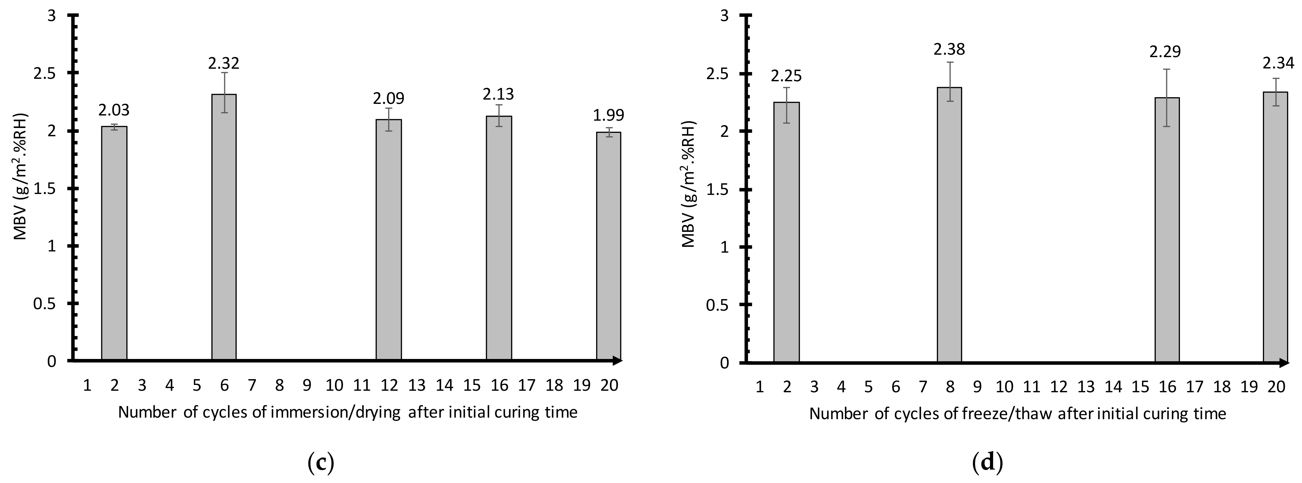
3.8.3. Evolution after Immersion–Drying Cycles

As was the case for the conservation under reference conditions, it should be noted that, for the samples that underwent immersion–drying cycles, the mean MBV (Figure 17c) evolves very little. It can be observed that the mean MBV of the studied samples equals around 2 kg/m².%RH, i.e., 2.03 kg/m².%RH after 2 cycles, 2.32 kg/m².%RH after 6 cycles, 2.09 kg/m².%RH after 12 cycles, 2.13 kg/m².%RH after 16 cycles and 1.99 kg/m².%RH after 20 cycles. With this value range, the mean MBV of these hemp concrete samples lies within the “excellent” category of materials for MBV, which includes all materials over 2 kg/m².%RH. These values are entirely similar to those obtained during the initial campaign; it is thus logical to conclude aging has no impact on this property.

3.8.4. Evolution after Freeze–Thaw Cycles

For this aging type, as in natural outdoor conservation, the mean MBV seems to increase compared to the initial campaign value (Figure 17d). It is apparent that the mean MBV of the studied samples lies above 2 kg/m².%RH, i.e., 2.25 kg/m².%RH after 2 cycles, 2.38 kg/m².%RH after 8 cycles, 2.29 kg/m².%RH after 16 cycles and 2.34 kg/m².%RH after 20 cycles. With this value range, the mean MBV of these hemp concrete samples lies in the “excellent” category of materials for MBV, which includes all materials over 2 kg/m².%RH. As with natural outdoor conservation, since the observed mean MBV is increasing, it may be concluded that this type of aging has an impact on this particular property, reflected by an increase; however, this conclusion must be taken with caution. As in natural outdoor exposure, the values obtained, for the most part, remain within the initial campaign measurement error range.

4. Conclusions

This paper highlighted a physical and hygrothermal characterization of hemp concrete. It was divided into three parts, with the main findings of each part being listed below:

-

In the first part, the spatial variability in thermal conductivity over a hemp beam was assessed. It was found that variability can be observed in the hemp beam’s length and height. One component of variability evolves randomly in space, while the other is likely to be directly tied to the manufacturing method. Indeed, this latter variability type is based on a layer-by-layer characterization; for the lower layer, a standard deviation differential of at least 0.005 W/m.K was found with the other layers.

-

In the second part, a univariate variability characterization campaign was performed. A linear relationship between density and thermal conductivity was obtained, as corroborated by the literature. Moreover, the inaccuracy of the Hot Disk method for thermal capacity characterization was highlighted, and a wide range of water vapor diffusion values could be observed, directly owing to the material microstructure.

-

The last and most important part of this paper was devoted to characterizing the samples during aging campaigns. Reference samples were held in a climate chamber, and three aging protocols were proposed: natural outdoor aging, immersion–drying, and freeze–thaw. The natural outdoor aging lasted 4 months, while cycle-based aging lasted 20 cycles. One key finding is that the reference sample properties were found to be rather constant during the entire conservation period. In contrast, major differences were uncovered depending on the properties and aging type that were considered. Hence, an increasing mass evolution was observed across all aging protocols; this was mainly due to the resumption of binder hydration. Only freeze–thaw loading actually changed the volume and density properties of the studied samples. As for thermal conductivity, a similar curve shape as that of mass (vs. time) could be observed for both aging protocols, which is quite logical given the theoretical link existing between these properties for this type of material. Lastly, the tested hygric properties revealed different behaviors. For all aging protocols, the water vapor permeability value increased, whereas a mostly constant MBV was found. Consequently, aged hemp concretes are able to remain in the top range of “good” or even “excellent” hygric regulators according to the NORDTEST protocol.

References

1. The United Nations Environment Programme. 2022 Global Alliance for Buildings and Construction. Global Status Report for Buildings and Construction: Towards a Zero-Emissions, Efficient and Resilient Buildings and Construction Sector—Executive Summary; The United Nations Environment Programme: Nairobi, Kenya, 2022. [Google Scholar]
2. Climate Change 2022 Impacts, Adaptation and Vulnerability, Summary for Policymakers; International Panel on Climate Change (IPCC): Geneva, Switzerland, 2022.
3. Louis, B.; Roche, C.; Talon, S.; Froment, S.; Saby, L. Réduire L’impact Carbone des Bâtiments, Cerema. 2021. Available online: https://publications.cerema.fr/webdcdc/pti-essentiel/impact-carbone-batiment/datas/pdf/Reduire_impact_batiment.pdf (accessed on 17 April 2023).
4. Beccali, M.; Cellura, M.; Fontana, M.; Longo, S.; Mistretta, M. Energy Retrofit of a Single-Family House: Life Cycle Net Energy Saving and Environmental Benefits. Renew. Sustain. Energy Rev. 2013, 27, 283–293. [Google Scholar] [CrossRef]
5. Rossi, B.; Marique, A.-F.; Glaumann, M.; Reiter, S. Life-Cycle Assessment of Residential Buildings in Three Different European Locations, Basic Tool. Build. Environ. 2012, 51, 395–401. [Google Scholar] [CrossRef]
6. Sartori, I.; Hestnes, A.G. Energy Use in the Life Cycle of Conventional and Low-Energy Buildings: A Review Article. Energy Build. 2007, 39, 249–257. [Google Scholar] [CrossRef]
7. Van Ooteghem, K.; Xu, L. The Life-Cycle Assessment of a Single-Storey Retail Building in Canada. Build. Environ. 2012, 49, 212–226. [Google Scholar] [CrossRef]
8. Karimpour, M.; Belusko, M.; Xing, K.; Bruno, F. Minimising the Life Cycle Energy of Buildings: Review and Analysis. Build. Environ. 2014, 73, 106–114. [Google Scholar] [CrossRef]
9. Ip, K.; Miller, A. Life Cycle Greenhouse Gas Emissions of Hemp–Lime Wall Constructions in the UK. Resour. Conserv. Recycl. 2012, 69, 1–9. [Google Scholar] [CrossRef]
10. Lecompte, T.; Levasseur, A.; Maxime, D. Lime and Hemp Concrete LCA: A Dynamic Approach of GHG Emissions and Capture. Acad. J. Civ. Eng. 2017, 35, 513–521. [Google Scholar] [CrossRef]
11. Pretot, S.; Collet, F.; Garnier, C. Life Cycle Assessment of a Hemp Concrete Wall: Impact of Thickness and Coating. Build. Environ. 2014, 72, 223–231. [Google Scholar] [CrossRef]
12. Evrard, A. Transient Hygrothermal Behavior of Lime-Hemp Materials. Ph.D. Thesis, Ecole Polytechnique de Louvain, Louvain, Belgium, 2008. [Google Scholar]
13. Tran Le, A.D.; Maalouf, C.; Mai, T.H.; Wurtz, E.; Collet, F. Transient Hygrothermal Behaviour of a Hemp Concrete Building Envelope. Energy Build. 2010, 42, 1797–1806. [Google Scholar] [CrossRef]
14. Nguyen, T.T.; Picandet, V.; Carre, P.; Lecompte, T.; Amziane, S.; Baley, C. Effect of compaction on mechanical and thermal properties of hemp concrete. Eur. J. Environ. Civ. Eng. 2010, 14, 545–560. [Google Scholar] [CrossRef]
15. Niyigena, C.; Amziane, S.; Chateauneuf, A. Assessing Variability of Hemp Concrete Properties during Experimental Tests: A Focus to Specimens’ Number. Acad. J. Civ. Eng. 2019, 37, 270–278. [Google Scholar] [CrossRef]
16. Benmahiddine, F.; Bennai, F.; Cherif, R.; Belarbi, R.; Tahakourt, A.; Abahri, K. Experimental Investigation on the Influence of Immersion/Drying Cycles on the Hygrothermal and Mechanical Properties of Hemp Concrete. J. Build. Eng. 2020, 32, 101758. [Google Scholar] [CrossRef]
17. Castel, Y.; Amaziane, S.; Sonebi, M. Durabilité du Béton de Chanvre: Résistance aux Cycles D’immersionhydrique et Séchage; IéreèConférenceEuroMaghrébine des BioComposites, BioComposites: Toulouse, France, 2016. [Google Scholar]
18. Sonebi, M.; Wana, S.; Amziane, S.; Khatib, J. Investigation of the Mechanical Performance and Weathering of Hemp Concrete. Acad. J. Civ. Eng. 2015, 33, 416–421. [Google Scholar] [CrossRef]
19. Maaroufi, M.; Bennai, F.; Belarbi, R.; Abahri, K. Experimental and Numerical Highlighting of Water Vapor Sorption Hysteresis in the Coupled Heat and Moisture Transfers. J. Build. Eng. 2021, 40, 102321. [Google Scholar] [CrossRef]
20. Benmahiddine, F.; Belarbi, R.; Berger, J.; Bennai, F.; Tahakourt, A. Accelerated Aging Effects on the Hygrothermal Behaviour of Hemp Concrete: Experimental and Numerical Investigations. Energies 2021, 14, 7005. [Google Scholar] [CrossRef]
21. Benmahiddine, F.; Belarbi, R. Effect of Immersion/Freezing/Drying Cycles on the Hygrothermal and Mechanical Behaviour of Hemp Concrete. Constr. Technol. Archit. 2022, 1, 555–562. [Google Scholar] [CrossRef]
22. Ismail, B. Contribution au Développement et Optimisation d’un Système Composite Biosourcé-Enduit de Protection pour L’isolation Thermique de Bâtiment. Ph.D. Thesis, Université d’Orléans, Orléans, France, 2020. [Google Scholar]
23. Walker, R.; Pavia, S.; Mitchell, R. Mechanical Properties and Durability of Hemp-Lime Concretes. Constr. Build. Mater. 2014, 61, 340–348. [Google Scholar] [CrossRef]
24. Chabannes, M.; Garcia-Diaz, E.; Clerc, L.; Bénézet, J.C. Studying the Hardening and Mechanical Performances of Rice Husk and Hemp-Based Building Materials Cured under Natural and Accelerated Carbonation. Constr. Build. Mater. 2015, 94, 105–115. [Google Scholar] [CrossRef]
25. Delannoy, G. Durabilité D’isolants à Base de Granulats Végétaux. Ph.D. Thesis, Université Paris-Est, Paris, France, 2018. [Google Scholar]
26. Marceau, S.; Glé, P.; Guéguen-Minerbe, M.; Gourlay, E.; Moscardelli, S.; Nour, I.; Amziane, S. Influence of Accelerated Aging on the Properties of Hemp Concretes. Constr. Build. Mater. 2017, 139, 524–530. [Google Scholar] [CrossRef]
27. Chamoin, J. Optimisation des Propriétés (Physiques, Mécaniques et Hydriques) de Bétons de Chanvre par la Maîtrise de la Formulation. Ph.D. Thesis, INSA Rennes, Rennes, France, 2013. [Google Scholar]
28. Merve Tuncer, H.; Canan Girgin, Z. Hemp Fiber Reinforced Lightweight Concrete (HRLWC) with Coarse Pumice Aggregate and Mitigation of Degradation. Mater. Struct. 2023, 56, 59. [Google Scholar] [CrossRef]
29. Ziane, S.; Khelifa, M.-R.; Mezhoud, S. A Study of the Durability of Concrete Reinforced with Hemp Fibers Exposed to External Sulfatic Attack. Civ. Environ. Eng. Rep. 2020, 30, 158–184. [Google Scholar] [CrossRef]
30. Viel, M.; Collet, F.; Lecieux, Y.; Marc, F.; Colson, V.; Lanos, C.; Hussain, A.; Lawrence, M. Évaluation de La Durabilité de Matériaux de Construction Biosourcés. Acad. J. Civ. Eng. 2019, 36, 60–63. [Google Scholar] [CrossRef]
31. Lawrence, M.; Jiang, Y. Porosity, Pore Size Distribution, Micro-structure. In Bio-Aggregates Based Building Materials: State-of-the-Art Report of the RILEM Technical Committee 236-BBM; Sofiane, A., Collet, F., Eds.; Springer: Dordrecht, The Netherlands, 2017. [Google Scholar] [CrossRef]
32. Technical Sheet of the Tradical PF 70. Available online: https://www.weber-tradical.com/wp-content/uploads/2018/03/fiche-technique-Tradical-PF-70.pdf (accessed on 9 April 2023).
33. Youssef, A.; Picandet, V.; Lecompte, T.; Challamel, N. Comportement du Béton de Chanvre en Compression Simple et Cisaillement; Rencontres Universitaires de Génie Civil: Bayonne, France, 2015. [Google Scholar]
34. Lo, Y.; Lee, H.M. Curing Effects on Carbonation of Concrete Using a Phenolphthalein Indicator and Fourier-Transform Infrared Spectroscopy. Build. Environ. 2002, 37, 507–514. [Google Scholar] [CrossRef]
35. Gustavsson, M.; Karawacki, E.; Gustafsson, S.E. Thermal conductivity, thermal diffusivity, and specific heat of thin samples from transient measurements with hot disk sensors. Rev. Sci. Instrum. 1994, 65, 3856–3859. [Google Scholar] [CrossRef]
36. Rode, C.; Peuhkuri, R.H.; Mortensen, L.H.; Hansen, K.K.; Time, B.; Gustavsen, A.; Ojanen, T.; Ahonen, J.; Svennberg, K.; Arfvidsson, J.; et al. (Eds.) Moisture Buffering of Building Materials; Technical University of Denmark, Department of Civil Engineering: Kongens Lyngby, Denmark, 2005. [Google Scholar]
37. Collet-Foucault, F. Caractérisation Hydrique et Thermique de Matériaux de Génie Civil à Faibles Impacts Environnementaux. Ph.D. Thesis, Insa Rennes, Rennes, France, 2004. [Google Scholar]
38. Glouannec, P.; Collet, F.; Lanos, C.; Mounanga, P.; Pierre, T.; Poullain, P.; Pretot, S.; Chamoin, J.; Zaknoune, A. Propriétés physiques de bétons de chanvre. Matériaux Tech. 2011, 99, 657–665. [Google Scholar] [CrossRef]
39. NF EN ISO 12572; Hygrothermal Performance of Building Materials and Products—Determination of Water Vapour Transmission Properties—Cup Method. AFNOR: Saint-Denis, France, 2016.
40. Viel, M.; Collet, F.; Lanos, C. Chemical and Multi-Physical Characterization of Agro-Resources’ by-Product as a Possible Raw Building Material. Ind. Crops Prod. 2018, 120, 214–237. [Google Scholar] [CrossRef]
41. Gourlay, E.; Glé, P.; Marceau, S.; Foy, C.; Moscardelli, S. Effect of Water Content on the Acoustical and Thermal Properties of Hemp Concretes. Constr. Build. Mater. 2017, 139, 513–523. [Google Scholar] [CrossRef]
42. Collet, F.; Chamoin, J.; Pretot, S.; Lanos, C. Comparison of the Hygric Behaviour of Three Hemp Concretes. Energy Build. 2013, 62, 294–303. [Google Scholar] [CrossRef]
43. Fourmentin, M. Impact de la Répartition et des Transferts d’eau sur les Propriétés des Matériaux de Construction à Base de Chaux Formulées. Ph.D. Thesis, Université de Paris Est, Paris, France, 2015. [Google Scholar]
Figure 1. Zones characterized for the thermal conductivity on the beam face (top view): (a) diagram of the characterized zones (top view); (b) photograph taken during characterization.
Buildings 13 02414 g001
Figure 2. Meteorological conditions during the natural outdoor aging of samples: (a) daily extreme temperatures; (b) daily precipitation amount.
Buildings 13 02414 g002
Figure 3. Mass and spatial dimensional measurements: (a) mass; (b) spatial dimension.
Buildings 13 02414 g003
Figure 4. Hot Disk set-up for thermal property characterization: (a) before characterization; (b) during characterization.
Buildings 13 02414 g004
Figure 5. Hygric property characterization: (a) sample for the MBV test; (b) set-up for the water vapor permeability test.
Buildings 13 02414 g005
Figure 6. Spatial variability characterization of thermal conductivity on the beam face.
Buildings 13 02414 g006
Figure 7. Variability of the thermal properties of samples after initial curing: (a) thermal conductivity; (b) heat capacity.
Buildings 13 02414 g007
Figure 8. Variability in sample MBV after the initial curing: (a) MBV variability; (b) MBV classification.
Buildings 13 02414 g008
Figure 9. Variability of water vapor permeability and equivalent thickness of water vapor permeability in the samples after initial curing: (a) water vapor permeability; (b) equivalent air thickness for water vapor permeability.
Buildings 13 02414 g009
Figure 10. Dry mass evolution of samples (in %) compared to the value obtained after initial characterization: (a) held as a reference; (b) natural outdoor retention; (c) immersion–drying; (d) freeze–thaw.
Buildings 13 02414 g010
Figure 11. Evolution in sample carbonation rate (%) through aging: (a) reference conservation; (b) natural outdoor conservation; (c) immersion–drying; (d) freeze–thaw.
Buildings 13 02414 g011
Figure 12. Evolution in sample carbonation through aging: (a) reference conservation; (b) natural outdoor conservation; (c) immersion–drying; (d) freeze–thaw.
Buildings 13 02414 g012
Figure 13. Dry volume evolution of samples (%) compared to the values obtained after initial characterization: (a) reference conservation; (b) natural outdoor conservation; (c) immersion–drying; (d) freeze–thaw.
Buildings 13 02414 g013aBuildings 13 02414 g013b
Figure 14. Dry density evolution of samples (%) compared to the value obtained after initial characterization: (a) reference conservation; (b) freeze–thaw cycles.
Buildings 13 02414 g014
Figure 15. Dry thermal conductivity evolution of samples (%) compared to the value obtained after initial characterization: (a) reference conservation; (b) natural outdoor conservation; (c) immersion–drying; (d) freeze–thaw.
Buildings 13 02414 g015
Figure 16. Water vapor permeability evolution of samples (%) compared to the value obtained after initial characterization: (a) reference conservation; (b) natural outdoor conservation; (c) immersion–drying; (d) freeze–thaw.
Buildings 13 02414 g016
Figure 17. MBV evolution of samples (%) compared to the value obtained after initial characterization: (a) reference conservation; (b) natural outdoor conservation; (c) immersion–drying; (d) freeze–thaw.
Buildings 13 02414 g017aBuildings 13 02414 g017b