Structural Damage Identification Based on Convolutional Neural Networks and Improved Hunter–Prey Optimization Algorithm

Abstract

Accurate damage identification is of great significance to maintain timely and prevent structural failure. To accurately and quickly identify the structural damage, a novel two-stage approach based on convolutional neural networks (CNN) and an improved hunter–prey optimization algorithm (IHPO) is proposed. In the first stage, the cross-correlation-based damage localization index (CCBLI) is formulated using acceleration and is input into the CNN to locate structural damage. In the second stage, the IHPO algorithm is applied to optimize the objective function, and then the damage severity is quantified. A numerical model of the American Society of Civil Engineers (ASCE) benchmark frame structure and a test structure of a three-storey frame are adopted to verify the effectiveness of the proposed method. The results demonstrate that the proposed approach is effective in locating and quantifying structural damage precisely regardless of noise perturbations. In addition, the reliability of the proposed approach is evaluated using a comparison between it and approaches based on CNN or the IHPO algorithm alone. The comparison results indicate that in single and multiple damage events, the proposed two-stage damage identification approach outperforms the other two approaches on the accuracy, and the average consumption time is 20% less than the method using the IHPO algorithm alone. Therefore, this paper provides a guideline for the study of high-accuracy and quick damage identification using both data-based and model-based hybrid methods.

1. Introduction

Structural health monitoring (SHM), including long-term and real-time monitoring, can timely detect structural damage, which is of great significance to avoid sudden failures and ensure the reliability of structures. Over the past decades, it has been widely explored and applied in civil engineering [1,2]. Furthermore, structural damage identification (SDI), as a key issue in SHM, has received extensive attention. When damage occurs, the material and geometric characteristics of the structures will change, affecting their strength, stiffness, and stability. Conventional damage identification methods are local methods, which cannot easily detect the damage inside structures and are not efficient for complex structures. Therefore, as global SHM techniques, vibration-based damage identification methods have been extensively used for SDI [3,4].

The vibration-based damage identification methods can be categorized into data-based and model-based approaches [5,6]. For the former, the commonly used methods are machine learning [7], deep learning [8], wavelet transform [9], and time series analysis [10], etc. These methods do not require finite element models (FEMs), which can avoid modeling errors. Nevertheless, the large amounts of data will cause difficulties in the data processing. Moreover, damage severity cannot be accurately quantified in most cases. For the latter, the main approaches include optimization algorithms-based [11] and Bayesian inference-based [12] model updating, etc. Although these model-based approaches can accurately locate the damage and quantify its severity, establishing accurate FEMs is extremely difficult, and modeling errors are inevitable.

Convolutional neural networks (CNN), as one of the representative data-based methods, can solve complex pattern classification and regression problems in practical engineering [13]. They have the characteristics of local connection, weight sharing, and down-sampling, which can greatly reduce network parameters and model complexity, as well as prevent over-fitting [14]. At present, they have been extensively applied to vibration-based SDI. Lin et al. [15] used a CNN to extract features from acceleration data of a simply supported beam, and accurately identify damage location using both a noise-free and a noisy data set. Abdeljaber et al. [16] proposed a CNN-based method of the damage localization using acceleration signals and verified its effectiveness by monitoring the main steel frame of the Qatar University grandstand simulator. Subsequently, an enhanced CNN-based method, which learns optimal features of signals to maximize the classification accuracy by the CNN, was proposed and precisely estimated the health condition of the American Society of Civil Engineers (ASCE) benchmark structure [17]. Azimi and Pekcan [18] utilized a CNN to extract the features of acceleration response, and then compressed the response data of a discrete histogram to effectively locate damage for frame structures. To summarize, CNN has an excellent performance in feature extraction and great potential in dealing with massive data in SDI [19]. Although the CNN-based method can robustly detect the occurrence and location of structural damage owing to the outstanding classification ability of CNNs, the structural damage severity can hardly be accurately quantified.

The optimization algorithms-based model updating method is the most representative model-based method. It transforms the damage detection problem into a mathematical optimization problem, and then to solve the problem by some optimization algorithms [20,21]. Based on this theory, numerous optimization algorithms are employed to identify damage, which can usually locate and quantify damage accurately. Dinh-Cong et al. [22] applied the Jaya algorithm to locate and quantify the damage for a two-dimensional frame, a planar truss, and a four-storey structure. Tran-Ngoc et al. [23] used the cuckoo search (CS) algorithm to identify the damage of a steel beam. Gomes et al. [24] adopted the sunflower optimization (SFO) algorithm to identify damage of the composite laminated plates. In addition, a series of creative ideas were developed to improve or enhance the basic algorithms, which can get a better optimization result. Wei et al. [25] introduced a disturbance in the evolution process to propose an improved particle swarm optimization (IPSO), and identified the damage of a beam, a truss, and a plate. Huang et al. [26] imported the Euclidean distance into the position updating formula to present the enhanced moth–flame optimization (EMFO) for SDI. Three numerical examples and two laboratory examples were applied to verify the proposed method. Ding et al. 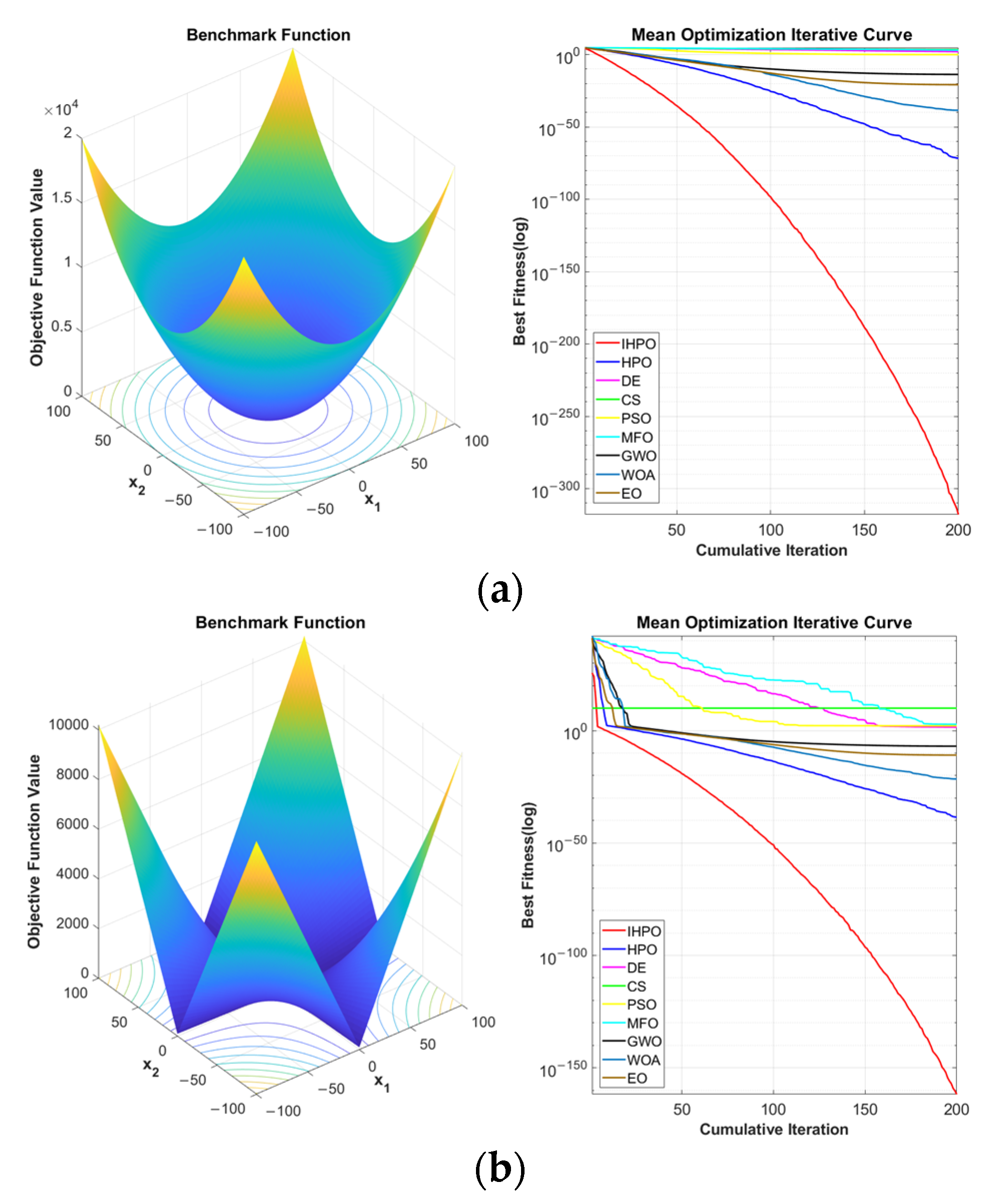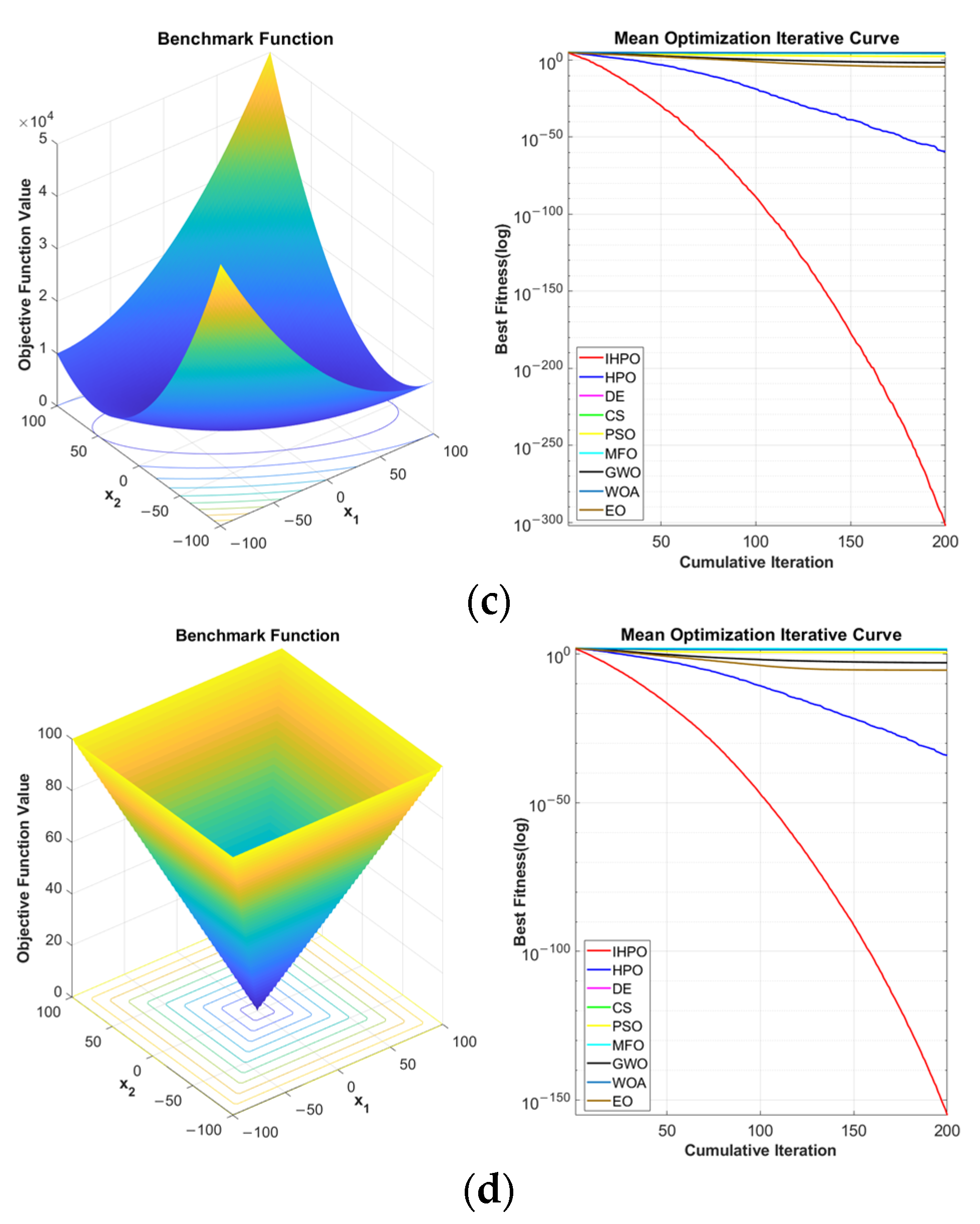[27] introduced a new search mode and the Gaussian search mode to the exploration and exploitation stages of the artificial bee colony algorithm, respectively. Then, a truss, a cantilevered plate, and a cracked beam are employed to verify the efficiency of the proposed modified artificial bee colony (MABC) algorithm. Although those optimization algorithms can detect the location and severity of the damage, the computational costs are extremely high. As the search space increases, the complexity increases sharply, especially when those optimization algorithms are applied to large-scale structures with numerous degrees of freedom, the iterative analysis will be complex and time-consuming.

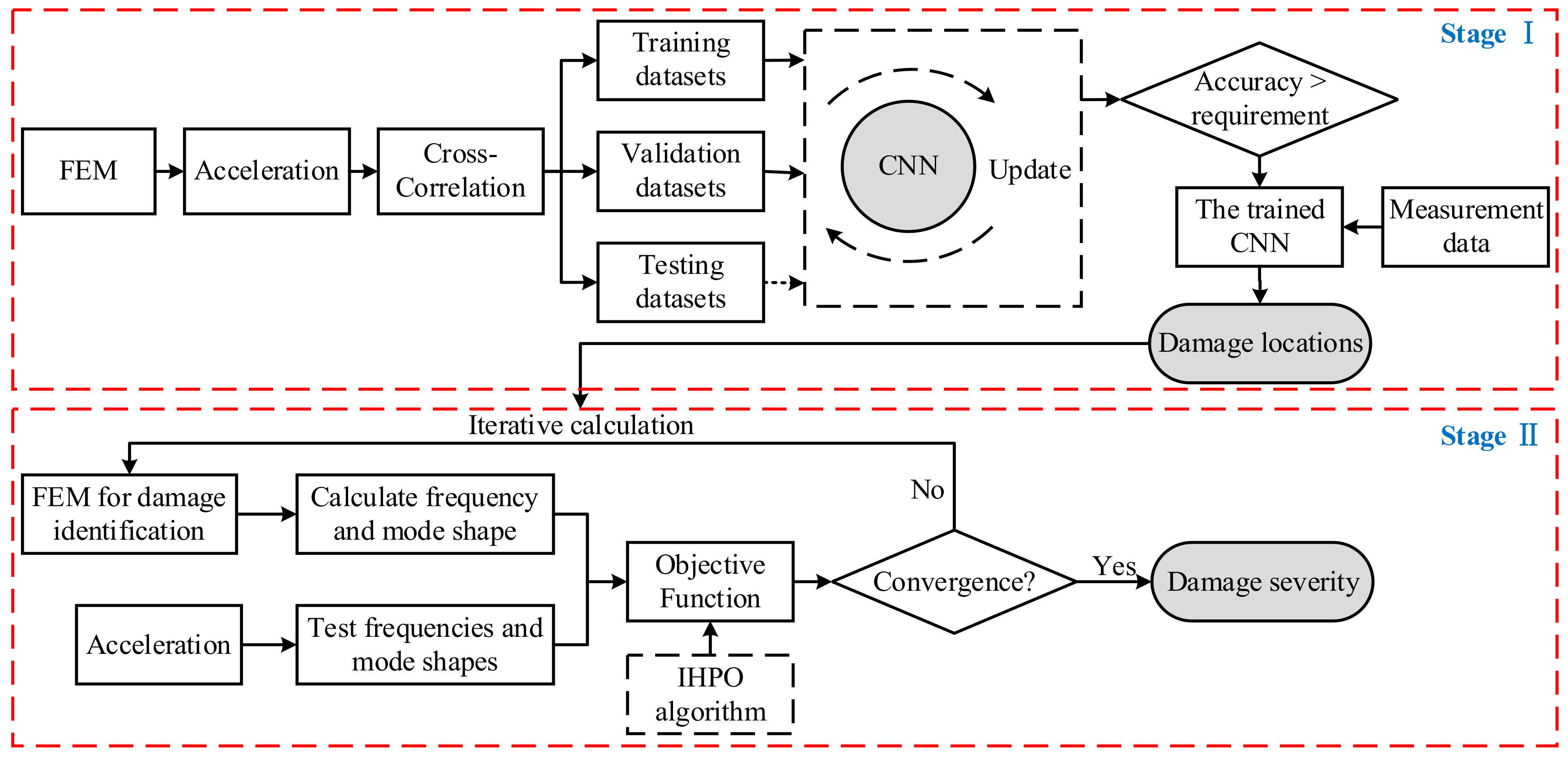
Therefore, in order to locate damage and quantify its severity accurately, as well as save computational costs effectively, it is promising to combine data-based methods and model-based methods. In addition, the hunter–prey optimization (HPO) algorithm is an effective intelligent optimization algorithm, which has the advantages of a fast convergence speed and a strong optimization ability and has great potential for structural damage identification. Based on the above-mentioned consideration, in this paper, a new two-stage damage identification approach based on CNN and an improved hunter–prey optimization (IHPO) algorithm has been first proposed. In the first stage, the cross-correlation-based damage localization index (CCBLI) is extracted from the acceleration responses, and then the CCBLI is input into CNN to locate structural damage. In the second stage, the IHPO algorithm is applied to optimize the objective function, and then to quantify the damage severity. A numerical example of the ASCE benchmark frame and a test structure of a three-storey frame with different damage cases are employed to investigate its accuracy and efficiency.

The remainder of this paper is organized as follows. In Section 2, firstly, the basic theories of cross-correlation and a CNN, which is combined with the CCBLI to locate structural damage, are presented. Secondly, the HPO algorithm and objective function are described in detail. At the same time, in order to improve the global optimization ability of the HPO algorithm, the tent chaos mapping, Cauchy distribution, and linear combination are adopted to modify it, and the IHPO algorithm is proposed. Then, the IHPO algorithm is employed to quantify the damage severity. In Section 3, a numerical example of the ASCE benchmark frame is applied to verify the feasibility of the proposed method. In Section 4, a test structure of a three-storey frame is employed to validate the applicability of the proposed approach. In Section 5, some conclusions of this paper are summarized.

2. Structural Damage Identification Based on CNN and IHPO Algorithm

2.1. Structural Damage Localization (SDL)

2.1.1. Cross-Correlation-Based Damage Localization Index (CCBLI)

The differential equation of undamped free vibration can be shown as follows:

$$M\ddot{x}+Kx=0$$

(1)

where $M$ and $K$ represent the mass and stiffness matrix of structures, respectively; $x$ and $\ddot{x}$ are the structural displacement and acceleration, respectively.

Cross-correlation is a measure of the similarity between two functions, that is, the correlation degree between continuous random signals $f_i(t)$ and $f_j(t)$ at any two different moments $t$ and $t+\tau$, which can be defined as follows:

$$R_{ij}(\tau )=\underset{T\to \infty }{\lim }\frac{1}{T}{\displaystyle {\int }_0^T{f}_i}(t)f_j(t+\tau )dt i,j\in 1,2,3\dots ,n$$

(2)

where $T$ denotes the measurement time of signal; $\tau$ is the time lag; $n$ means the number of sensors; $f_i(t)$ and $f_j(t)$ represent the acceleration at the i-th and j-th locations, respectively [28,29].

Similarly, for discrete functions, the cross-correlation can be calculated between i-th and j-th locations as follows:

$$R_{ij}(m)=\left\{\begin{array}{c}\frac{1}{N-m}{\displaystyle \sum _{n=0}^{N-m-1}{f}_i(x+m)f_j(x),m\ge 0}\\ R_{ij}(-m),m<0\end{array}\right.$$

(3)

where $N$ denotes the number of the acceleration data, $N>m$; and $\Delta t$ is sampling period, $\tau =m\times \Delta t$.

It can be seen that the $R_{ij}$ measures the similarity between the two acceleration responses, and $R_{ij}\in [0,1]$. When the two acceleration responses series are similar to each other, $R_{ij}$ is close to 1. If the structure is damaged, the $R_{ij}^D$ of the damaged structure is different from $R_{ij}^U$ of the undamaged structure. Therefore, the structural damage can be detected by the cross-correlation of acceleration. The damage localization index (CCBLI) can be defined as follows:

$$CCBL{I}_{ij}=R_{ij}^D$$

(4)

2.1.2. Convolutional Neural Networks (CNN)

Convolutional neural networks (CNN) are mainly composed of the input layer, the convolution layer, the pooling layer, the fully connected layer, and the output layer. Compared with the traditional neural network, it has the characteristics of local connection, weight sharing, and down-sampling. It can effectively reduce the network parameters, prevent over-fitting, and improve the efficiency of extracting local features. In recent years, it has been widely used in structural damage identification (SDI).

(1)

Convolutional Layer

The convolution layer is the core of the CNN, and the local feature extraction is realized by connecting the input of each neuron to the local sensing region of the previous layer. The convolution operation can be categorized into convolution and activation, and the calculation process can be shown as follows:

$$T=f_k({\displaystyle \sum _{x,y,z=1}^r{C}_{x,y,z}}{w}_{x,y,z}{}^s+b^s)$$

(5)

where $C$ and $T$ denote the input and output of the convolution layer, respectively; $r$ and $s$ stand for the serial number of convolution kernels and the number of channels, respectively; $w$ and $b$ represent the weights and biases of the convolution kernel; $f_k$ means the activation function of the k-th layers; and $x$, $y$, and $z$ are dimensions of input data.

In the activation operation, a nonlinear function such as Sigmoid, Tanh, ReLU, and Leaky ReLU is adopted to map the input after linear transformation, to enhance the nonlinear expression ability of the network. Among them, the ReLU eliminates the gradient vanishing effect of the Sigmoid function, and the gradient calculation speed is very fast, so it has been widely used. Therefore, the ReLU is applied to the convolution layer in this paper.

(2)

Pooling Layer

The pooling layer is the feature mapping layer, which reduces the output dimension of the convolution layer to realize the down-sampling of local information and effectively prevent over-fitting. The max pooling, average pooling, and overlapping pooling are the common pooling methods. In this paper, the max pooling is adopted to express local features, and multiple convolutions and pooling layers are used to realize feature extraction.

(3)

Fully connected Layer

In the fully connected layer, each neuron is fully connected to all neurons in the front layer, and the predicted value is calculated by weighted summation of inter-layer weight coefficients. For regression processes, the nonlinear activation functions such as ReLU, Tanh and Sigmoid are not applicable to the last fully connected layer. Because they map the output in the range of [0, ∞), (−1, 1), and (0, 1), respectively. Therefore, to improve the expression ability of the model, the ReLU and the linear activation function are adopted to the fully connected layer and output layer, respectively.

2.1.3. The Proposed CNN for SDL

A 2D-CNN framework programed in MATLAB is established for SDL, and its overall architecture is shown in Figure 1. The CCBLI is input into the CNN, and the multiple convolution and pooling operations are utilized to realize feature extraction. Then, they are expanded and input to the fully connected layer, and mapped to the structural damage through the regression layer.

2.2. Structural Damage Quantification (SDQ)

2.2.1. The Original Hunter–Prey Optimization Algorithm

Hunter–prey optimization (HPO) is a new intelligent optimization algorithm proposed by Naruei et al. [30] in 2022. It has the advantages of fast convergence and a strong optimization ability by simulating the animal hunting process. The original HPO algorithm randomly initializes the population position in the solution space, and the population initialization formula can be shown as follows:

$$x_i=rand(1,d)\times (ub-lb)+lb$$

(6)

where $x_i$ means the position of the i-th hunter or prey, $i=1,2,\dots ,N$, $N$ represents the population size; $lb$ and $ub$ are the lower and upper bounds of the search space, respectively; $rand(1,d)$ is the random numbers of [0, 1], $d=1,2,\dots ,D$, and $D$ denotes the dimension of the search space. The hunter location update formula can be expressed as follows:

$$x_{i,j}(t+1)=x_{i,j}(t)+0.5[(2CZ{P}_{pos(j)}-x_{i,j}(t)+2(1-C)Z{\mu }_{(j)}-x_{i,j}(t))]$$

(7)

where $x(t)$ and $x(t+1)$ mean the current and the next iteration location of hunters; $P_{pos}$ stands for the location of the prey; $\mu =\frac{1}{n}{\displaystyle \sum _{i=1}^n{x}_i}$ represents the average of all locations; $Z$ is the adaptive parameter calculated by Equation (9):

$$P=r_1<CIDX=(P==0)$$

(8)

$$Z=r_2\otimes IDX+r_3\otimes (~IDX)$$

(9)

where $r_1$ and $r_3$ are random vectors of [0, 1]; $P$ is a random vector with a value of 0 or 1; $r_2$ is a random number within [0, 1]; $IDX$ is the index value of the vector $r_1$ satisfying the conditions $(P==0)$; and $C$ represents the balance parameter between exploration and exploitation, and its value decreases from 1 to 0.02 in the iterative process. The calculation can be shown as follows:

$$C=1-it(\frac{0.98}{I{t}_{\max }})$$

(10)

where $it$ and $I{t}_{\max }$ represent the current iteration number and the maximum iteration number, respectively. According to Equation (11), the Euclidean distance from the average position of each searched individual can be presented as follows:

$$D_{euc(i)}={({\displaystyle \sum _{j=1}^d{(x_{i,j}-{\mu }_{i,j})}^2})}^{\frac{1}{2}}$$

(11)

Search agents with the largest distance from the average position $\mu$ are regarded as prey $P_{pos}$:

$$P_{pos}=x_i|i is index of Max(end)sort(D_{euc})$$

(12)

If the maximum distance between the search agent and the average position $\mu$ is considered in each iteration, the convergence of the algorithm is poor. In the actual hunting scene, when the prey is captured, the hunter will move to the new prey location next time. The decreasing mechanism is conducted to simulate this scenario, as shown in Equation (13).

$$kbest=round(C\times n)$$

(13)

where $n$ is the number of search agents. At the beginning of the algorithm, $kbest=N$. During the algorithm iteration, the hunter selects the search agent farthest from the average position as the prey and attacks it, and the $kbest$ gradually decreases. At the end of the algorithm, the $kbest$ is equal to the first search agent (the shortest distance from the average position). Therefore, the prey position calculation Equation (12) can be changed to Equation (14):

$$P_{pos}=x_i|i is sorted D_{euc}(kbest)$$

(14)

When the prey is attacked, it will try to escape to the global optimal position, so that it has better survival opportunities, and the hunter will choose another prey. Thus, the prey position update formula can be established as follows:

$$x_{i,j}(t+1)=T_{pos(j)}+CZ\cos (2\pi r_4)\times (T_{pos(j)}-x_{i,j}(t))$$

(15)

where $x(t)$ and $x(t+1)$ mean the current position and the next iteration position of the prey, respectively; $T_{pos}$ is the global optimal position; $r_4$ is a random number within [−1, 1]; and the function $\cos (\cdot )$ and its input parameters make the next prey position at different radii and angles of the global optimal position.

Combining Equations (7) and (15), the updated formulation of hunter or prey position can be selected as follows:

$$x_{i,j}(t+1)=\left\{\begin{array}{c}{x}_{i,j}(t)+0.5[(2CZ{P}_{pos(j)}-x_{i,j}(t))+(2(1-C)Z{\mu }_{(j)}-x_{i,j}(t))], r_5<\beta (a)\\ T_{pos(j)}+CZ\cos (2\pi r_4)\times (T_{pos(j)}-x_{i,j}(t)), r_5\ge \beta (b)\end{array}\right.$$

(16)

where $r_5$ is the random number within [0, 1]; and $\beta =0.1$ means the adjusting parameter. If $r_5<\beta$, the search agent is regarded as a hunter, the location update formula is (16a); and if $r_5\ge \beta$ the search agent is regarded as the prey, the location update formula is (16b).

2.2.2. The Improved Hunter–prey Optimization (IHPO) Algorithm

(1)

Tent Chaos Mapping and Cauchy Distribution

A high-quality initial population is helpful to improve the optimization performance of the algorithm. However, random initialization is adopted by the HPO algorithm, which is difficult to guarantee the initial population quality. The chaotic mapping has the characteristics of randomness, ergodicity, and order, which can ensure population diversity [31]. Therefore, in this paper, the sequence generated by the tent chaos is applied to initialize the population, so as to enhance the population diversity and improve the convergence speed in the early stage. The expression of the tent mapping can be shown as follows:

$$y_{i+1}^{}=\left\{\begin{array}{c}\eta y_i^{}, 0\le y_i^{}\le 0.5 \\ \eta (1-y_i^{}), 0.5\le y_i^{}\le 1 \end{array}\right.$$

(17)

where $i$ is the corresponding particle number, $i=1, 2, \dots , N$; $\eta \in (0,2]$ stands for the chaotic parameter, which is proportional to the chaos. In this paper, $\eta =2$.

In addition, the random variables subject to Cauchy distribution are introduced in Equation (17) to solve the problem of small period and unstable period points and ensure the three properties of the tent mapping sequence. Thus, the initial value based on the tent mapping and Cauchy distribution can be calculated as follows:

$$y_{i+1}^{}=\left\{\begin{array}{c}\mu y_i^{}+cauchy(0,1)\times \frac{1}{N}, 0\le y_i^{}\le 0.5 \\ \mu (1-y_i^{})+cauchy(0,1)\times \frac{1}{N}, 0.5\le y_i^{}\le 1 \end{array}\right.$$

(18)

The initial population is obtained by introducing Equation (18) into Equation (6), which can be expressed as follows:

$$x_i=y_i\times (ub-lb)+lb$$

(19)

(2)

Linear Combination

In addition, in the original HPO algorithm, the hunter only updates the current position according to the average position and prey position, and the algorithm is prone to fall into the local optimum. To increase the hunter’s search space and improve the global search ability of the algorithm, the global optimal position $T_{pos(j)}$ is introduced into the position updating formula. Meanwhile, the prey position and the average position are linearly combined with the global optimal position $\frac{(P_{pos(j)}-T_{pos(j)})}{2}$ and $\frac{({\mu }_{(j)}-T_{pos(j)})}{2}$, respectively, to replace the $P_{pos}$ and ${\mu }_{(j)}$ in Equation (7).

Furthermore, in the original HPO algorithm, the prey only updates the current position through the global optimal position, and the search range of the algorithm is limited. To increase the search range of the prey and improve the exploitation ability of the algorithm, the linear combination between the local optimal position and the global optimal position $\frac{(gbes{t}_{(j)}-T_{pos(j)})}{2}$ is introduced into Equation (15) to replace the $T_{pos(j)}$. Searching the global optimal in the early stage becomes more likely. Therefore, the new location update formula can be summarized as follows:

$$x_{i,j}(t+1)=\left\{\begin{array}{c}{x}_{i,j}(t)+0.5[(2CZ\frac{(P_{pos(j)}-T_{pos(j)})}{2}-x_{i,j}(t))+(2(1-C)Z\frac{({\mu }_{(j)}-T_{pos(j)})}{2}-x_{i,j}(t))], r_5<\beta (a)\\ T_{pos(j)}+CZ\cos (2\pi r_4)\times \left(\frac{(gbes{t}_{(j)}-T_{pos(j)})}{2}-x_{i,j}(t)\right), r_5\ge \beta (b)\end{array}\right.$$

(20)

(3)

The flowchart of IHPO algorithm

After introducing those improvements into the original HPO algorithm, the flowchart of IHPO algorithm can be illustrated in Figure 2.

2.2.3. Optimization Performance Evaluation of IHPO Algorithm

In this section, several test functions are adopted to evaluate the optimization performance of the IHPO algorithm. Meanwhile, the IHPO has been compared with other algorithms, such as the differential evolution (DE) algorithm [32], cuckoo search (CS) [23], particle swarm optimization (PSO) [25], moth–flame optimization (MFO) [26], the grey wolf optimizer (GWO) [33], the whale optimization algorithm (WOA) [34], and the equilibrium optimizer (EO) [35]. The population size and iteration number of each algorithm are 100 and 200, respectively. Other specific parameters are listed as follows: (1) DE: cross probability 0.015; (2) CS: discovery probability 0.25; and (3) PSO: learning rate $c_1=c_2=2$; maximum and minimum of inertia weight are 0.9 and 0.4, respectively. Each algorithm is repeated 10 times until reaching the max iteration. The average statistical results and iterative curves of the aforementioned algorithms are illustrated in

Table 1. The statistical results of four test functions.

Function Formula	Algorithm	Best	Worst	Mean	Std
$\begin{array}{l}{f}_1(x)={\displaystyle \sum _{i=1}^{10}{x}_i^2}\\ x_i\in \left[-100,100\right]\end{array}$	IHPO	0	1.31 × 10−317	1.32 × 10−318	0
	HPO	2.76 × 10−78	2.20 × 10−71	2.40 × 10−72	6.92 × 10−72
	DE	7.03 × 10	1.65 × 102	1.22 × 102	2.54 × 10
	CS	1.32 × 103	3.26 × 103	2.23 × 103	5.32 × 102
	PSO	3.96 × 10−1	1.85	9.76 × 10−1	5.41 × 10−1
	MFO	4.34 × 102	1.82 × 103	1.00 × 103	4.75 × 102
	GWO	8.71 × 10−16	4.07 × 10−14	2.07 × 10−14	1.32 × 10−14
	WOA	1.62 × 10−43	2.86 × 10−38	3.23 × 10−39	8.96 × 10−39
	EO	−1.28 × 10−11	1.02 × 10−11	4.97 × 10−13	6.31 × 10−12
$\begin{array}{l}{f}_2(x)={\displaystyle \sum _{i=1}^{10}\left|x_i\right|}+{\displaystyle \prod _{i=1}^{10}\left|x_i\right|}\\ x_i\in \left[-10,10\right]\end{array}$	IHPO	4.02 × 10−166	1.54 × 10−161	1.68 × 10−162	4.97 × 10−162
	HPO	4.45 × 10−41	1.98 × 10−38	2.93 × 10−39	6.01 × 10−39
	DE	2.98 × 10	4.29 × 10	3.57 × 10	3.52
	CS	1.00 × 1010	1.00 × 1010	1.00 × 1010	0
	PSO	2.16 × 10	2.46 × 102	1.30 × 102	7.26 × 10
	MFO	4.83 × 102	9.47 × 102	6.62 × 102	1.28 × 102
	GWO	6.08 × 10−8	2.05 × 10−7	1.20 × 10−7	5.95 × 10−8
	WOA	5.73 × 10−24	2.10 × 10−21	3.07 × 10−22	6.39 × 10−22
	EO	−7.39 × 10−13	1.04 × 10−12	7.67 × 10−14	5.90 × 10−13
$\begin{array}{l}{f}_3(x)={{\displaystyle \sum _{i=1}^{10}\left({\displaystyle \sum _{j-1}^i{x}_j}\right)}}^2\\ x_i\in [-100,100]\end{array}$	IHPO	1.0 × 10−310	5.33 × 10−302	5.44 × 10−303	0
	HPO	3.59 × 10−72	5.00 × 10−59	5.69 × 10−60	1.57 × 10−59
	DE	2.76 × 104	3.98 × 104	3.30 × 104	3.92 × 103
	CS	1.15 × 104	1.87 × 104	1.49 × 104	2.14 × 103
	PSO	6.73 × 10	7.48 × 102	2.45 × 102	2.20 × 102
	MFO	1.21 × 104	3.34 × 104	2.26 × 104	7.50 × 103
	GWO	5.33 × 10−4	6.02 × 10−2	2.00 × 10−2	2.00 × 10−2
	WOA	2.63 × 104	4.89 × 104	4.07 × 104	7.37 × 103
	EO	−2.15 × 10−3	2.13 × 10−3	1.17 × 10−4	1.20 × 10−3
$\begin{array}{l}{f}_4(x)=\underset{i}{\max \left\{\left|x_i\right|,1\le i\le 10\right\}}\\ x_i\in [-100,100]\end{array}$	IHPO	2.60 × 10−158	2.98 × 10−155	8.46 × 10−156	1.13 × 10−155
	HPO	1.02 × 10−36	4.90 × 10−34	8.45 × 10−35	1.53 × 10−34
	DE	4.81 × 10	5.81 × 10	5.33 × 10	3.46
	CS	3.57 × 10	4.23 × 10	3.94 × 10	2.04
	PSO	2.08	5.05	3.16	9.59 × 10−1
	MFO	4.49 × 10	6.76 × 10	5.53 × 10	7.24
	GWO	4.85 × 10−4	2.28 × 10−3	1.18 × 10−3	6.06 × 10−4
	WOA	1.59 × 10−2	7.88 × 10	2.49 × 10	2.47 × 10
	EO	−8.36 × 10−6	1.41 × 10−6	−3.11 × 10−6	2.75 × 10−6

and Figure 3.

It can be seen from Table 1 that the convergence result of the IHPO algorithm is smaller than that of the other algorithms for each test function. As can be seen from Figure 3, the convergence speed of the IHPO algorithm is significantly faster than the other algorithms. In summary, the IHPO algorithm outperforms in the global optimization ability, convergence efficiency, and convergence accuracy, having greater potential for SDQ.

2.2.4. The Objective Function of SDQ

The characteristic equation of a structure can be shown as follows:

$$\left(K-{\omega }_i^{2}M\right){\varphi }_i=0 i=1,2,\dots ,n$$

(21)

where ${\omega }_i$ and ${\varphi }_i$ stand for the first i-th natural frequencies and mode shapes, respectively; and $n$ is the total degree of freedom (DOF).

Cosine similarity measures correlation by the cosine value of the angle between two vectors [36]. So, the cosine similarity of the measured and calculated mode shapes can be shown as follows:

$$\cos ({\phi }_i^t,{\phi }_i^c)=\frac{{({\phi }_i^t)}^T{\phi }_i^c}{\left|{\phi }_i^t\right|\left|{\phi }_i^c\right|}$$

(22)

where ${\phi }_i^t$ and ${\phi }_i^c$ are the first i-th measured and calculated mode shapes, respectively; and $\cos ({\phi }_i^t,{\phi }_i^c)\in [-1,1]$. Then, the square of cosine similarity can be calculated as follows:

$${\cos }^2({\phi }_i^t,{\phi }_i^c)={\left(\frac{{({\phi }_i^t)}^T{\phi }_i^c}{\left|{\phi }_i^t\right|\left|{\phi }_i^c\right|}\right)}^2=\frac{{({({\phi }_i^t)}^T{\phi }_i^c)}^2}{({({\phi }_i^t)}^T{\phi }_i^t)({({\phi }_i^c)}^T{\phi }_i^c)}=MAC({\phi }_i^t,{\phi }_i^c)$$

(23)

It can be seen from Equation (23) that the ${\cos }^2({\phi }_i^t,{\phi }_i^c)$ is equal to the modal assurance criteria (MAC). Therefore, the high-power of the cosine similarity can be defined as the damage index:

$$CSBI({\phi }_i^t,{\phi }_i^c)={\left(\frac{{({\phi }_i^t)}^T{\phi }_i^c}{\left|{\phi }_i^t\right|\left|{\phi }_i^c\right|}\right)}^R=MA{C}^{\frac{R}{2}}({\phi }_i^t,{\phi }_i^c)$$

(24)

The Equation (24) shows that the larger $R$, the more sensitive $CSBI$ to damage than $MAC$. Moreover, the square of the frequency residuals has a better sensitivity to local damage. Therefore, the objective function is built based on the $CSBI$ and the square of the frequency residuals, which can be determined as follows:

$$F=c_1{{\displaystyle \sum _{i=1}^n\left(\frac{{\omega }_i^t-{\omega }_i^c}{{\omega }_i^t}\right)}}^2+c_2{\displaystyle \sum _{i=1}^n\frac{{\left(1-\sqrt{CSB{I}_i}\right)}^2}{CSB{I}_i}}$$

(25)

where ${\omega }_i^t$ and ${\omega }_i^c$ are the i-th measured and calculated frequencies, respectively; the $c_1$ and $c_2$ mean the weighted coefficient of frequencies and mode shapes, respectively, and $c_1=1$, $c_2=0.1$ is taken in this paper [37]; and $n=4$ is the modal order; the power in $CSBI$ is $R=4$.

2.3. Damage Identification Based on CNN and IHPO Algorithm

In this subsection, combining the data-based method (CNN) and model-based method (IHPO algorithm), a novel two-stage damage identification method is proposed, which can accurately and quickly identify structural damage. The main steps of the proposed damage identification method are listed as follows:

(1)

The CCBLI is calculated according to the acceleration responses;

(2)

The CNN is adopted to construct the mapping relationship between the CCBLI and the corresponding damage location;

(3)

The measured data of a practical engineering structure is fed to the trained CNN for locating structural damage approximately;

(4)

The IHPO algorithm is used to optimize the objective function, to accurately estimate the damage severity.

The flowchart of damage identification is shown in Figure 4.

3. Numerical Example

A damage identification benchmark structure, as shown in Figure 5, was proposed by the American Society of Civil Engineers (ASCE). This is a 4-storey 2-span × 2-span steel frame model. The plane size and the height of each layer are 2.5 m × 2.5 m and 0.9 m, respectively. Each floor contains 9 column members, 12 beam members, and 8 diagonal bracing members. The section of beam, column, and diagonal bracing are S75 × 11, B100 × 9, and L25 × 25 × 3, respectively. Hot rolled 300 W grade steel (nominal yield strength 300 Mpa) is used for the members. The other related information can be referred to Refs. [38,39,40]. The numerical model and the labels of columns based on MATLAB can be shown in Figure 5. The measured DOFs of acceleration, as shown in Figure 5 by red arrows, are located at No. 2, 4, 6, and 8 columns.

3.1. Damage Localization

3.1.1. Data Generation for Training

In this subsection, the 16 elements (the red ones 2, 4, 6, 8, 31, 33, 32, 37, 60, 62, 64, 66, 89, 91, 93, 95) numbered in Figure 5 are taken as the research objects and named as 1, 2, …, 16 in turn. The structural damage is introduced by the reduction of elements stiffness, and the maximum damaged element number is three. Therefore, there are $C_{16}^1=16$, $C_{16}^2=120$, and $C_{16}^3=560$ damage locations for single-site, double-site, and three-site damage case, respectively. Each damage location is calculated 3000, 400, and 350 times for single-site, double-site, and three-site damage case, respectively. The range of stiffness reduction is random and the uniform distribution within [0, 0.8]. Thus, there are 48,000, 48,000, and 196,000 datasets for single-site damage case, double-site damage case, and three-site damage case, respectively.

The Gaussian noise is applied at the middle of each floor in the y-direction to excite the system, and the state space method is used to calculate acceleration. The sampling frequency and sampling time are 1000 Hz and 40 s, respectively. Consequently, the CCBLI can be calculated by the measured acceleration data to detect damage. Meanwhile, to verify the feasibility and robustness of the proposed method, the measurement noise can be simulated as follows:

$$y_i^{\prime }=y_i(1+\eta {\zeta }_i)$$

(26)

where $y_i$ and $y_i^{\prime }$ represent the i-th original and polluted acceleration, respectively; $\eta$ means the degree of noise, 1%, 3%, and 5% are considered, respectively; and ${\zeta }_i$ is a random number in the range of [−1, 1].

The input data of CNN are formed by CCBLI with a size of 16 × 16, and the output is a vector of structural stiffness reduction with a size of 16 × 1. In order to reduce the computational cost of the network, the datasets of three damage cases are mixed to train the CNN. The CCBLI is fed into the CNN for feature learning, and then the learned features are mapped to a vector of structural stiffness reduction, to locate damage.

3.1.2. Performance Evaluation of the CNN Model

The datasets are randomly divided into three parts: 80% for training, 10% for validation, and 10% for testing. All hyper-parameters are selected based on the validation loss. The initial learning rate is 10⁻⁴, decaying 0.5 factors per 20 epochs. The mini-batch size of the neural network is 50, and it performs 200 epochs with the Adam optimizer. The training loss curves are shown in Figure 6. It can be observed that the convergency performance of the training loss of clean datasets consistently outperforms the noisy datasets. The performance degrades gradually with the noise level increase, which conforms to reality.

Moreover, the loss value of validation datasets, as well as the mean square error (MSE) and regression value (R, 0 ≤ R ≤ 1) of the test datasets are utilized to quantitatively evaluate the performance of the trained model. To summarize, the smaller loss and MSE, whereas the higher R, and the higher accuracy of the trained model. The performance evaluation results of the trained model are presented in

Table 2. Performance evaluation results.

Noise Level (%)	Validation Loss	Test MSE	Test R
-	0.877	0.044	0.943
1	0.906	0.055	0.941
3	1.061	0.078	0.891
5	1.285	0.091	0.830

From Table 2, it can be seen that when clean datasets are used, the performance of the trained model is the best, and the final validation loss is 0.877; the test MSE and test R values are 0.04 and 0.94, respectively. The performance degrades slightly as the noise level increases. When the noise level of 5% is considered, the corresponding evaluation results are 1.285, 0.091, and 0.830, respectively. In summary, the trained CNN model based on the CCBLI has the potential for providing an accurate SDL.

3.1.3. Damage Localization Results

Furthermore, three damage cases, as shown in

Table 3. Damage cases of the ASCE benchmark frame.

Noise Level (%)	Damage Case	Damage Element	Damage Severity (%)
-, 3, 5 and 10	Case 1	#1	20
	Case 2	#4, #9	10, 60
	Case 3	#5, #11 and #14	30, 20 and 70

, are utilized to demonstrate the SDL performance of the trained CNN. The damage identification results and the corresponding errors are illustrated in Figure 7.

It can be seen that it is inaccurate to detect damage using the CNN. First of all, with the increase in damaged elements and noise level, the number of false alarms will increase. Secondly, in all damage cases, the damage quantification results are worse with the maximum identification error of 30%. Consequently, a novel two-stage damage identification method is proposed in this paper, that is, in the first stage, the CCBLI is input into the CNN to locate damage; in the second stage, the IHPO algorithm is used to estimate the damage severity. Therefore, the damage localization results of the ASCE benchmark frame can be obtained from Figure 7, as shown in

Table 4. Damage localization results of the ASCE benchmark frame.

Noise Level (%)	Damage Case	True Damage Severity#Element	Suspected Damage Element
-	Case 1	20%#1	#1
	Case 2	10%#4 and 60%#9	#4 and #9
	Case 3	30%#5, 20%#11 and 70%#14	#5, #11 and #14
1	Case 1	20%#1	#1
	Case 2	10%#4 and 60%#9	#4 and #9
	Case 3	30%#5, 20%#11 and 70%#14	#5, #11 and #14
3	Case 1	20%#1	#1
	Case 2	10%#4 and 60%#9	#3, #4 and #6
	Case 3	30%#5, 20%#11 and 70%#14	#4, #5, #11, #12 and #16
5	Case 1	20%#1	#1
	Case 2	10%#4 and 60%#9	#3, #4, #5 and #9
	Case 3	30%#5, 20%#11 and 70%#14	#4, #5, #62, #64, #66 and #91

. Here, the element whose value (identification damage severity) exceeds the threshold (i.e., 5%), is selected as the suspected damage element.

It can be seen that when there is no noise, the damage in the three damage cases can be accurately located. The localization accuracy decreases with the increased amount of noise. In the most complex situation, namely, the three damaged elements and the 5% measurement noise are considered, and the number of damage variables has been reduced to 6. In summary, under the influence of noise, this method can also obtain reliable damage localization results. Therefore, the CCBLI as the input of the CNN has great effectiveness and robustness for single and multiple damage localization.

3.2. Damage Quantification

After locating the damage by the CNN in the first stage, the number of damage variables has been significantly reduced. Then, the first four natural frequencies and mode shapes are employed to construct the objective function, as shown in Equation (25). The damage severity of the suspected elements is put into the IHPO algorithm for optimization to quantify the damage. The population size and the iterative number are 200 and 100, respectively. This process is run 10 times. Figure 8 presents the average iterative curves obtained by the IHPO algorithm for double-element damage case. The average damage identification results and the corresponding errors are illustrated in Figure 9.

It can be observed that even considering the influence of noise, the convergence speed of the IHPO algorithm is very fast and has an excellent optimization effect. The actual damage severity can be detected successfully under all damage scenarios, there is no misjudgment phenomenon, and all the errors are less than 12%. These results demonstrate that the effectiveness and robustness of the IHPO algorithm in damage estimation. In addition, the feasibility of the proposed method has been verified again.

3.3. Comparative Study

Furthermore, to further verify the effectiveness of the proposed method, the proposed two-stage damage identification method (Method 1, data-based and model-based hybrid method) is compared with the method using the CNN (Method 2, data-based method) and the IHPO algorithm (Method 3, model-based method) alone. For this process, the key parameters are similar to the Section 3.1 and Section 3.2. Among them, the damage identification results of Method 2 can refer to Section 3.1. The comparative results of damage identification about Method 1 and Method 3 are shown in

Table 5. The comparative results of damage identification.

Noise Level (%)	Damage Case	Ture Damage	Method 1		Method 3
			Identified Damage	Time	Identified Damage	Time
-	Case 1	20%#1	19.95%#1	91.73	15.16%#1 and 5.37%#2	118.84
	Case 2	10%#4 and 60%#9	10.22%#4 and 60.19%#9	93.36	10.57%#4, 13.62%#9, 19.17%#12, 20.85%#13, and 9.35%#15	118.95
	Case 3	30%#5, 20%#11, and 70%#14	30%#5, 20%#11, and 70%#14	93.47	5.98%#5, 8.49%#8, 5.14%#9, 6.20%#10, 20%#11, 21.15%#14, and 18.20%#15	119.03
1	Case 1	20%#1	19.73%#1	94.83	13.96%#1 and 6.67%#2	119.63
	Case 2	10%#4 and 60%#9	9.60%#4 and 61.02%#9	96.08	6.38%#4, 9.13%#9, 13.42%#12, 21.0%#13, and 20.62%#16	119.66
	Case 3	30%#5, 20%#11, and 70%#14	30.01%#5, 19.98%#11, and 70%#14	96.10	5.40%#4, 7.91%#5, 5.01%#9, 6.19%#10, 5.31%#11, 5.26%#13, 16.42%#14, and 19.57%#15	120.37
3	Case 1	20%#1	19.62%#1	96.13	18.72%#2	119.78
	Case 2	10%#4 and 60%#9	10.98%#4 and 58.27%#9	97.84	10.52%#4, 5.90%#9, 12.45%#12, 38.77%#13, and 9.89%#16	120.30
	Case 3	30%#5, 20%#11, and 70%#14	30.48%#5, 18.94%#11, and 68.91%#14	97.75	8.53%#4, 20.75%#9, 18.05%#12, 12.32%#13, and 11.68%#16	120.36
5	Case 1	20%#1	19.58%#1	96.92	18.41%#2	120.27
	Case 2	10%#4 and 60%#9	11.16%#4 and 57.81%#9	97.63	8.06%#4, 15.31%#9, 19.17%#12, 6.60%#13, and 15.21%#16	120.47
	Case 3	30%#5, 20%#11, and 70%#14	30.76%#5, 18.81%#11, and 68.67%#14	98.08	8.56%#8, 5.61%#9, 7.35%#10, 6.29%#11, 5.23%#12, 6.13%#13, 12.57%#14, 16.27%#15, and 5.82%#16	121.42

.

Firstly, according to Section 3.1 (Figure 7) and Section 3.2 (Figure 9), it can be seen that in all cases, “Method 1” can obtain more accurate identification results without any false alarm than “Method 2”. Secondly, from the comparison results about Method 1 and Method 3, it can be observed that compared with “Method 3”, “Method 1” can not only accurately identify damage location and severity with no misjudgment phenomenon, but can also effectively reduce the calculation time. The average consumption time of “Method 1” is 20% less than that of “Method 3”. Because “Method 3” needs to optimize more variables than “Method 1”. Therefore, the data-based and model-based hybrid method can provide more accuracy for damage identification. In conclusion, the proposed two-stage damage identification method makes full use of the ability of the CNN to automatically extract features from massive data and the global optimization ability of the IHPO algorithm, which can reduce the search dimension of the algorithm, improve the efficiency and accuracy of damage identification, and then save the computational costs.

4. Experiment Validation

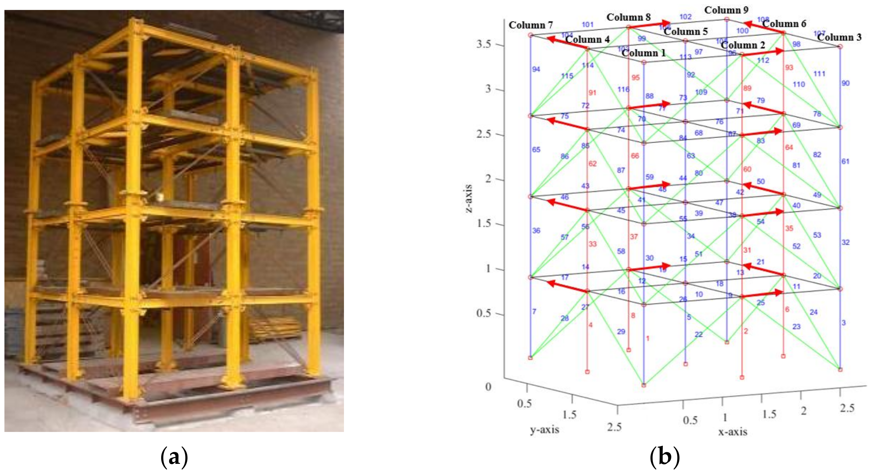
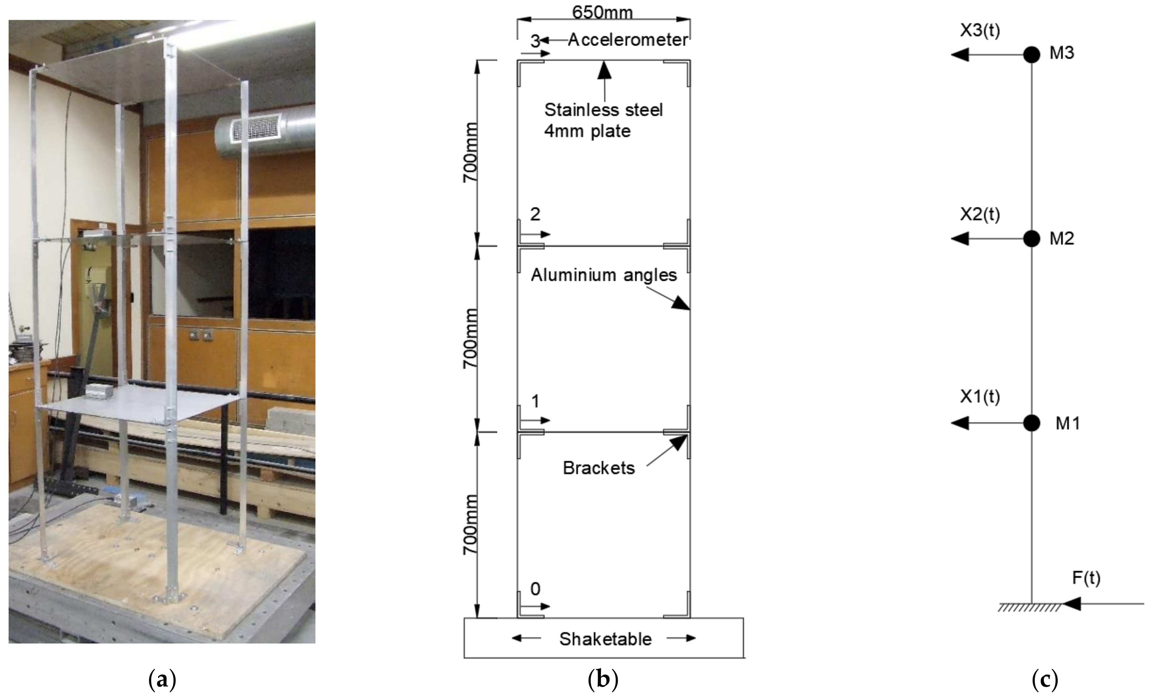
In this section, a three-storey frame structure [41], as shown in Figure 10, is adopted to further validate the effectiveness of the proposed approach. The structure consists of aluminum angle columns and stainless-steel floor plates, which are connected by bolted aluminum brackets. The lateral stiffness of each floor can be changed independently without permanently damaging the structure, which is achieved by easily replacing the columns with brackets. The thickness and size of the stainless-steel plates are 4.0 mm and 650 mm × 650 mm, respectively. The size and thickness of the equal angle columns are 30 mm × 30 mm and 4.5 mm. The column height of each floor is 0.7 m, and its ends are fixed on aluminum brackets with two bolts. The width and thickness of the bracket are 30 mm and 4.5 mm, respectively, and each bracket is fixed on the plate with two 6.0 mm bolts. The structure is mounted on 20 mm plywood and fixed on the vibration table with 10 mm bolts. Damage is introduced by replacing the original 4.5 mm thick column of a specific floor with a thinner 3.0 mm aluminum angle. The structural states are summarized in

Table 6. The structural states and labels.

Label	State	Damage Information
State 0	Undamaged	Baseline condition
State 1	Damaged	7% in 1st storey stiffness reduction
State 2	Damaged	10% in 2nd storey stiffness reduction
State 3	Damaged	7% and 10% in 1st and 2nd storey stiffness reduction, respectively

.

The structure is equipped with four 2.5 V/g uniaxial accelerometers, one for measuring table acceleration and the other for each floor, as shown in Figure 10. The acceleration in the direction of ground motion was measured at the sampling rate of 400 Hz. MATLAB was used to filter the data. The original signal was decreased from 400 Hz to 100 Hz. The detail of the sensors’ layout, test equipment, and test process can be referred to the Ref. [41].

4.1. The Updated Finite Element Model

In this paper, the test structure is simulated as three lumped masses by MATLAB, including beams connecting each lumped mass, as shown in Figure 10. The Young’s modulus and the density of aluminum are 71.7 GPa and 2700 kg/m³, respectively. Then, the IHPO algorithm is utilized for model updating based on the natural frequencies and mode shapes under the intact state. The updating results about frequencies and MACs of the experimental and numerical models are presented in

Table 7. The frequencies and MACs of experimental and numerical model.

Order	Experimental Frequency (Hz)	Frequency before Update (Hz)	Error (%)	MAC	Updated Frequency (Hz)	Error (%)	MAC
1	1.928	2.026	5.09	0.996	1.929	0.04	0.993
2	5.520	5.868	6.31	0.927	5.520	0.01	0.993
3	8.550	9.261	8.31	0.930	8.545	0.05	0.991

.

It can be seen that the errors between the updated frequencies and the measured ones are greatly reduced. The max error is only 0.05%, and the MACs are all greater than 0.99, which indicates that the updated FEM and experimental model have a good correlation. Therefore, the datasets generated from the updated FEM can be used for training the proposed CNN network, and the measured data collected from the laboratory tests are applied to identify damage.

4.2. Damage Localization

4.2.1. Data Generation for Training

Similarly, damage is introduced by reducing the elements stiffness. The maximum number of damaged elements is two. So, there are three damage locations for single-site and double-site damage cases. Each damage location is calculated 2000 times. The range of stiffness reduction is random and has uniform distribution within [0, 0.15], and 6000 datasets are collected for each damage case. Based on the updated FEM, the x-direction impact force is applied at the vibration table, as shown in Figure 10, to obtain the acceleration responses. Meanwhile, the sampling frequency and time are the same as the experimental. Then, the CCBLI can be obtained.

Accordingly, input the CCBLI with 3 × 3 to the CNN for feature learning and output the stiffness reduction vector with 3 × 1. In addition, the data split ratio, network architecture, and hyperparameters applied to train the network are the same as in Section 3.1.

4.2.2. Damage Localization Results

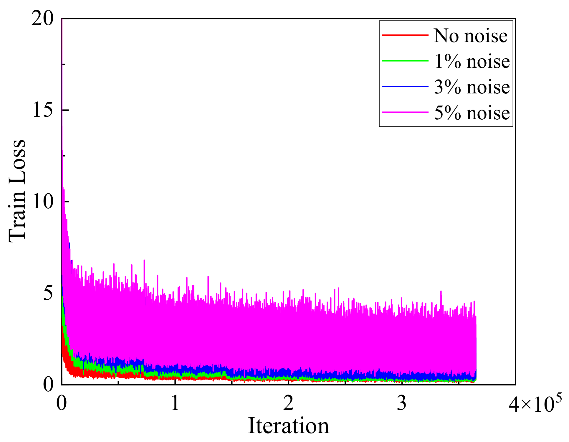
Figure 11 shows the training loss curve. It can be observed that the curve has a good convergence performance, and the ultimate validation loss is 0.685. Additionally, the trained model shows good performance with the MSE (0.046) and R value (0.947). These results indicate that the trained model has great potential for accurate SDL.

Furthermore, three damage cases in the laboratory test, i.e., State 1, 2, and 3, as shown in

Table 8. Damage localization results of three-storey frame.

Label	True Damage Severity#Element	Suspected Damage Element
State 1	7%#1	#1
State 2	10%#2	#2
State 3	7%#1 and 10%#2	#1 and #2

, are used to test the proposed approach. The corresponding CCBLI is input to the trained CNN to locate the damage. The results are shown in Table 8. It is shown that the proposed approach can accurately locate the single-site and multiple-site damage.

4.3. Damage Quantification

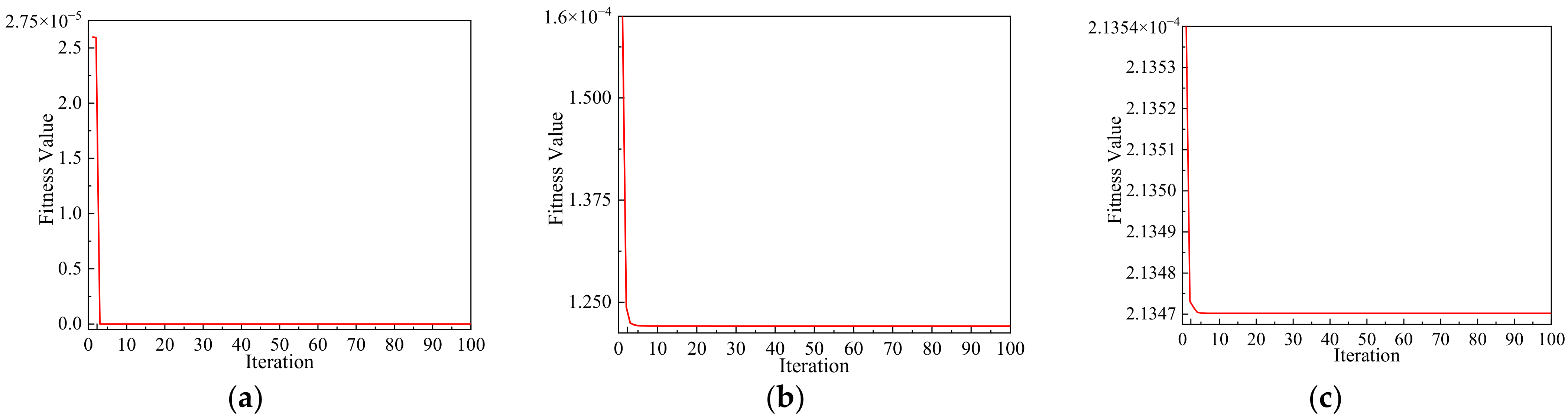
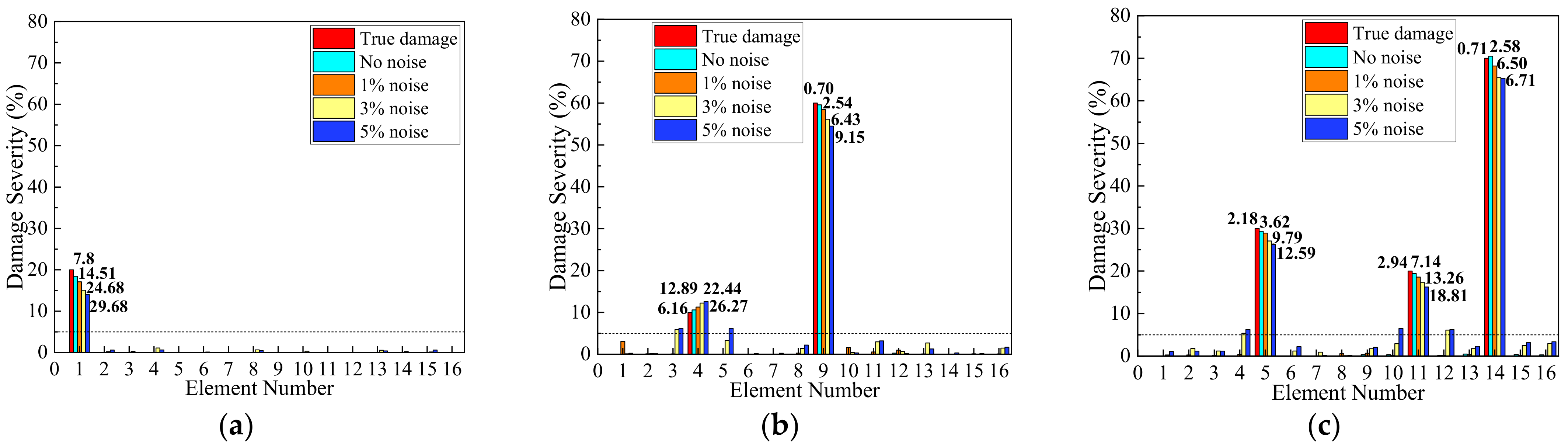
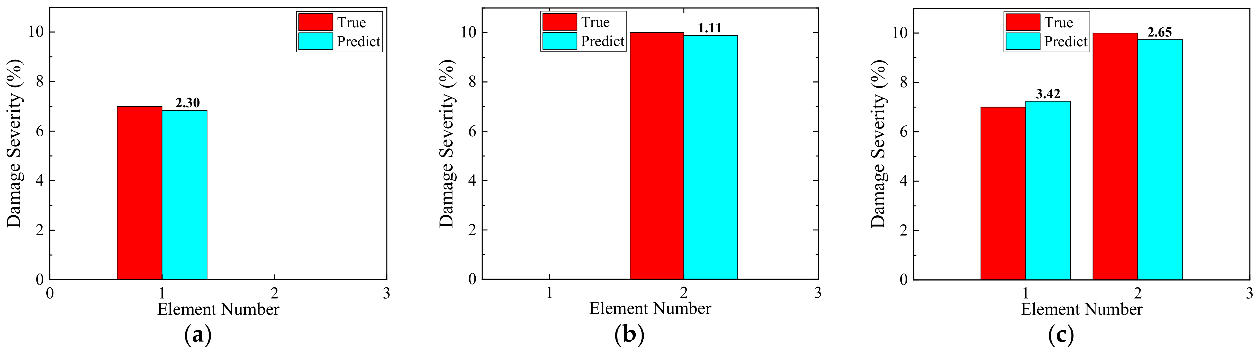
Next, based on the damage localization results obtained from the first stage, there are only 1, 1, and 2 variables for State 1, 2 and 3, respectively. Then, the first four modes are employed to solve the optimization problem in the second stage. For this progress, the parameters are the same as in Section 3.2. The iterative curves are presented in Figure 12. The average damage identification results and the corresponding errors are illustrated in Figure 13.

It can be observed that the IHPO algorithm performs with a fast convergence speed and a high convergence accuracy. The actual damage quantification can be detected successfully in all damage cases, and the identification errors are less than 4%. In summary, the experimental verification of the three damage cases illustrates that the proposed method can be applied to the practical application of SDI with sufficient accuracy.

5. Conclusions

This paper proposes a new two-stage approach based on convolutional neural networks (CNN) and an improved hunter–prey optimization (IHPO) algorithm, to improve the efficiency and accuracy of damage identification. In the first stage, the cross-correlation-based damage localization index (CCBLI) is input into the CNN to locate the potential damage effectively. In the second stage, the IHPO algorithm is adopted to accurately determine the damage severity. To investigate its accuracy and efficiency, a numerical example of the American Society of Civil Engineers (ASCE) benchmark frame and a test structure of a three-storey frame are employed with different damage cases. The results demonstrate that it has superior performance in identifying structural damage with noise corruption. There are several conclusions can be drawn as follows:

(1)

Compared with other common optimization algorithms, the IHPO algorithm has the advantages of a good global optimization capacity, a fast convergence speed, and a high convergence precision. It has great potential for structural damage quantification.

(2)

A numerical example of the ASCE benchmark frame structure considering measurement noise has been investigated, and the structural damage identification performance of the proposed method has been evaluated by making a comparison with the method using the CNN or the IHPO algorithm alone. The results show that in single-site and multiple-site damage identification, the proposed method outperforms the other two approaches on the accuracy and robustness. Moreover, the average consumption time is 20% less than the method using the IHPO algorithm alone. Therefore, this proposed two-stage damage identification approach can reduce the search dimension of the algorithm, improve the efficiency of damage identification, and save computation costs.

(3)

A test model of the three-storey frame structure is adopted to further investigate the feasibility of the proposed method. The results demonstrate that the proposed method has a good performance in detecting single-site and multiple-site damage and can be applied to the practical application of structural damage identification with sufficient accuracy.

(4)

Compared with the data-based and model-based methods, this study illustrates that the combination of a data-based method (CNN) and a model-based method (IHPO algorithm) can quickly identify damage accurately, which has great potential for practical structures. However, the numerical model and experimental example used in this paper are idealized without considering the influence of wind load, humidity variation, and environmental temperature fluctuation, et al. Therefore, these factors will be considered in future work to further test the effectiveness of the proposed method.

References

1. Gatti, M. Structural health monitoring of an operational bridge: A case study. Eng. Struct. 2019, 195, 200–209. [Google Scholar] [CrossRef]
2. Vazquez, B.; Esteban, G.; Gaxiola-Camacho Ramon, J.; Bennett, R.; Guzman-Acevedo, M.; Gaxiola-Camacho, I.E. Structural evaluation of dynamic and semi-static displacements of the Juarez Bridge using GPS technology. Measurement 2017, 110, 146–153. [Google Scholar] [CrossRef]
3. Huang, Y.; Shao, C.; Wu, B.; Beck, J.L.; Li, H. State-of-the-art review on Bayesian inference in structural system identification and damage assessment. Adv. Struct. Eng. 2019, 22, 1329–1351. [Google Scholar] [CrossRef]
4. Hou, R.; Xia, Y. Review on the new development of vibration-based damage identification for civil engineering structures: 2010-2019. J. Sound. Vib. 2021, 491, 115741. [Google Scholar] [CrossRef]
5. Huang, M.; Lei, Y.; Li, X.; Gu, J. Damage Identification of Bridge Structures Considering Temperature Variations-Based SVM and MFO. J. Aerospace Eng. 2021, 34, 04020113. [Google Scholar] [CrossRef]
6. Vagnoli, M.; Remenyte-Prescott, R.; Andrews, J. Railway bridge structural health monitoring and fault detection: State-of-the-art methods and future challenges. Struct. Health Monit. 2018, 17, 971–1007. [Google Scholar] [CrossRef]
7. Flah, M.; Nunez, I.; Ben Chaabene, W.; Nehdi, M. Machine learning algorithms in civil structural health monitoring: A systematic review. Arch. Comput. Method Eng. 2021, 28, 2621–2643. [Google Scholar] [CrossRef]
8. Rafiei, M.H.; Adeli, H. A novel unsupervised deep learning model for global and local health condition assessment of structures. Eng. Struct. 2018, 156, 598–607. [Google Scholar] [CrossRef]
9. Yang, Y.; Nagarajaiah, S. Blind identification of damage in time-varying systems using independent component analysis with wavelet transform. Mech. Syst. Signal Process. 2014, 47, 3–20. [Google Scholar] [CrossRef]
10. Gul, M.; Catbas, F. Structural health monitoring and damage assessment using a novel time series analysis methodology with sensor clustering. J. Sound Vib. 2011, 330, 1196–1210. [Google Scholar] [CrossRef]
11. Chen, Z.; Yu, L. A novel pso-based algorithm for structural damage detection using bayesian multi-sample objective function. Struct. Eng. Mech. 2017, 63, 825–835. [Google Scholar] [CrossRef]
12. Rogers, T.; Worden, K.; Fuentes, R.; Dervilis, N.; Tygesen, U.; Cross, E. A bayesian non-parametric clustering approach for semi-supervised structural health monitoring. Mech. Syst. Signal Process. 2018, 119, 100–119. [Google Scholar] [CrossRef]
13. Zheng, J.; Teng, X.; Liu, J.; Qiao, X. Convolutional Neural Networks for Water Content Classification and Prediction With Ground Penetrating Radar. IEEE Access 2019, 7, 185385–185392. [Google Scholar] [CrossRef]
14. LeCun, Y.; Bengio, Y.; Hinton, G. Deep learning. Nature 2015, 521, 436–444. [Google Scholar] [CrossRef] [PubMed]
15. Lin, Y.-z.; Nie, Z.-h.; Ma, H.-w. Structural Damage Detection with Automatic Feature-Extraction through Deep Learning: Structural damage detection with automatic feature-extraction through deep learning. Comput. Aided Civ. Inf. 2017, 32, 1025–1046. [Google Scholar] [CrossRef]
16. Abdeljaber, O.; Avci, O.; Kiranyaz, S.; Gabbouj, M.; Inman, D.J. Real-time vibration-based structural damage detection using one-dimensional convolutional neural networks. J. Sound. Vib. 2017, 388, 154–170. [Google Scholar] [CrossRef]
17. Abdeljaber, O.; Avci, O.; Kiranyaz, M.S.; Boashash, B.; Sodano, H.; Inman, D.J. 1-D CNNs for structural damage detection: Verification on a structural health monitoring benchmark data. Neurocomputing 2018, 275, 1308–1317. [Google Scholar] [CrossRef]
18. Azimi, M.; Pekcan, G. Structural health monitoring using extremely compressed data through deep learning. Comput. Aided Civ. Inf. 2020, 35, 597–614. [Google Scholar] [CrossRef]
19. Zhao, R.; Yan, R.; Chen, Z.; Mao, K.; Wang, P.; Gao, R.X. Deep learning and its applications to machine health monitoring. Mech. Syst. Signal Process. 2019, 115, 213–237. [Google Scholar] [CrossRef]
20. Dinh-Cong, D.; Vo-Duy, T.; Ho-Huu, V.; Dang-Trung, H.; Nguyen-Thoi, T. An efficient multi-stage optimization approach for damage detection in plate structures. Adv. Eng. Softw. 2017, 112, 76–87. [Google Scholar] [CrossRef]
21. Huang, M.; Lei, Y.; Cheng, S. Damage identification of bridge structure considering temperature variations based on particle swarm optimization-cuckoo search algorithm. Adv. Struct. Eng. 2019, 22, 3262–3276. [Google Scholar] [CrossRef]
22. Du, D.; Vinh, H.; Trung, V.; Hong Quyen, N.; Trung, N. Efficiency of Jaya algorithm for solving the optimization-based structural damage identification problem based on a hybrid objective function. Eng. Optimiz. 2018, 50, 1233–1251. [Google Scholar] [CrossRef]
23. Tran-Ngoc, H.; Khatir, S.; Roeck, G.D.; Bui-Tien, T.; Abdel Wahab, M. Damage assessment in beam-like structures using cuckoo search algorithm and experimentally measured data. In Proceedings of the 13th International Conference on Damage Assessment of Structures, Porto, Portugal, 9–10 July 2019; Springer: Singapore, 2020. [Google Scholar] [CrossRef]
24. Gomes, G.F.; Da Cunha, S.S.; Ancelotti, A.C. A sunflower optimization (SFO) algorithm applied to damage identification on laminated composite plates. Eng. Comput. Ger. 2019, 35, 619–626. [Google Scholar] [CrossRef]
25. Wei, Z.; Liu, J.; Lu, Z. Structural damage detection using improved particle swarm optimization. Inverse. Probl. Sci. Eng. 2018, 26, 792–810. [Google Scholar] [CrossRef]
26. Huang, M.; Li, X.; Lei, Y.; Gu, J. Structural damage identification based on modal frequency strain energy assurance criterion and flexibility using enhanced Moth-Flame optimization. Structures 2020, 28, 1119–1136. [Google Scholar] [CrossRef]
27. Ding, Z.; Fu, K.; Deng, W.; Li, J.; Zhongrong, L. A modified Artificial Bee Colony algorithm for structural damage identification under varying temperature based on a novel objective function. Appl. Math. Model. 2020, 88, 122–141. [Google Scholar] [CrossRef]
28. Dang, X. Statistic Strategy of Damage Detection for Composite Structure Using the Correlation Function Amplitude Vector. Procedia. Eng. 2015, 99, 1395–1406. [Google Scholar] [CrossRef]
29. Diwakar, C.M.; Patil, N.; Sunny, M.R. Structural Damage Detection Using Vibration Response Through Cross-Correlation Analysis: Experimental Study. AIAA J. 2018, 56, 2455–2465. [Google Scholar] [CrossRef]
30. Naruei, I.; Keynia, F.; Sabbagh Molahosseini, A. Hunter-prey optimization: Algorithm and applications. Soft. Comput. 2022, 26, 1279–1314. [Google Scholar] [CrossRef]
31. Demidova, L.A.; Gorchakov, A.V. A Study of Chaotic Maps Producing Symmetric Distributions in the Fish School Search Optimization Algorithm with Exponential Step Decay. Symmetry 2020, 12, 784. [Google Scholar] [CrossRef]
32. Reed, H.M.; Nichols, J.M.; Earls, C.J. A modified differential evolution algorithm for damage identification in submerged shell structures. Mech. Syst. Signal Process. 2013, 39, 396–408. [Google Scholar] [CrossRef]
33. Zare Hosseinzadeh, A.; Ghodrati Amiri, G.; Jafarian Abyaneh, M.; Seyed Razzaghi, S.A.; Ghadimi Hamzehkolaei, A. Baseline updating method for structural damage identification using modal residual force and grey wolf optimization. Eng. Optimiz. 2020, 52, 549–566. [Google Scholar] [CrossRef]
34. Mirjalili, S.; Lewis, A. The Whale Optimization Algorithm. Adv. Eng. Softw. 2016, 95, 51–67. [Google Scholar] [CrossRef]
35. Aval, S.B.B.; Mohebian, P. Joint Damage Identification in Frame Structures by Integrating a New Damage Index with Equilibrium Optimizer Algorithm. Int. J. Struct. Stab. Dyn. 2022, 22, 2250056. [Google Scholar] [CrossRef]
36. Ye, J. Cosine similarity measures for intuitionistic fuzzy sets and their applications. Math. Comp. Model. Dyn. 2011, 53, 91–97. [Google Scholar] [CrossRef]
37. Huang, M.-S.; Gül, M.; Zhu, H.-P. Vibration-Based Structural Damage Identification under Varying Temperature Effects. J. Aerospace Eng. 2018, 31, 04018014. Available online: https://xueshu.baidu.com/usercenter/paper/show?paperid=1f987dd604c5f94ac689965a2ebb3f47&site=xueshu_se (accessed on 17 July 2022). [CrossRef]
38. Johnson, E.A.; Lam, H.F.; Katafygiotis, L.S.; Beck, J.L. Phase I IASC-ASCE Structural Health Monitoring Benchmark Problem Using Simulated Data. J. Eng. Mech. 2004, 130, 3–15. [Google Scholar] [CrossRef]
39. Bernal, D.; Dyke, S.J.; Lam, H.F.; Beck, J.L. Phase II of the ASCE benchmark study on SHM. In Proceedings of the 15th ASCE Engineering Mechanics Conference, Columbia University, New York, NY, USA, 2–5 June 2002; Available online: http://authors.library.caltech.edu/34238/1/Report_bldg_shm_ana2.pdf (accessed on 17 July 2022).
40. Lam, H.F. PHASE Ile of the Iasc-Asce Benchmark Study on Structural Health Monitoring. In Proceedings of the A Conference & Exposition on Structural Dynamics, Kissimmee, FL, USA, 3–6 February 2003; Available online: https://repository.hkust.edu.hk/ir/Record/1783.1-28551 (accessed on 17 July 2022).
41. Omenzetter, P.; De Lautour, O.R. Detection of Seismic Damage in Buildings Using Structural Responses; Report number: UNI/535; Earthquake Commission Research Foundation: The Pines Beach, New Zealand, 2008. [CrossRef]
Figure 1. The proposed CNN for SDL (n: the number of acceleration sensors; n_ele: the number of elements).
Buildings 12 01324 g001
Figure 2. The flowchart of IHPO algorithm.
Buildings 12 01324 g002
Figure 3. The figures and iteration curves of four test functions. (a) f 1 ( x ) ; (b) f 2 ( x ) ; (c) f 3 ( x ) ; and (d) f 4 ( x ) .
Buildings 12 01324 g003aBuildings 12 01324 g003b
Figure 4. The flowchart of damage identification.
Buildings 12 01324 g004
Figure 5. ASCE benchmark frame (unit: m). (a) test structure; (b) numerical model.
Buildings 12 01324 g005
Figure 6. The training curves of ASCE benchmark frame.
Buildings 12 01324 g006
Figure 7. Damage identification results and corresponding errors using CNN. (a) Case 1; (b) Case 2; and (c) Case 3.
Buildings 12 01324 g007
Figure 8. The iterative curves for the ASCE benchmark frame.
Buildings 12 01324 g008
Figure 9. Damage identification results and corresponding errors for the ASCE benchmark frame. (a) Case 1; (b) Case 2; and (c) Case 3.
Buildings 12 01324 g009
Figure 10. Three-storey frame [41]. (a) test model; (b) diagram of accelerometer locations and external dimensions; (c) its simplified three DOF system.
Buildings 12 01324 g010
Figure 11. The training curves of three-storey frame.
Buildings 12 01324 g011
Figure 12. The iterative curves for the three-storey frame. (a) State 1; (b) State 2; and (c) State 3.
Buildings 12 01324 g012
Figure 13. Damage identification results and corresponding errors for the three-storey frame. (a) State 1; (b) State 2; and (c) State 3.
Buildings 12 01324 g013