1. Introduction
Over the past few years structural identification (SI) has become an intrinsic part of current civil engineering practice. This is due to the fact that accurate information coming from SI increases the level of knowledge of the structural behavior. SI usually is pursued processing vibrational measurements aiming to identify the main modal parameters: frequencies, shapes, and damping ratios. These parameters could be used to update a linear and elastic finite element model in order to make more reliable the numerical forecast model. Experimental Modal Analysis (EMA) [
1] and Operational Model Analysis (OMA) [
2] constitute two different methodologies to carry out SI. The former is an input–output technique that requires the knowledge of the input (usually an artificial load to excite the structure) and output (structural response) while the second is based only on the output measure.
In recent years, OMA techniques have had wider use because they do not need cumbersome instrumentation installed and, above all, the recording of measurements induced by ambient vibrations is sufficient (wind, traffic load, crowd). Among the various algorithms and procedures developed for performing SI by output-only data, Enhanced Frequency Domain Decomposition and Stochastic Subspace Identification are the most known and applied [
3,
4].
During the years, experimental dynamic and static analysis has increasingly been incorporated in civil engineering applications [
5]. Moreover, among all different typologies of non-destructive or minor-destructive tests [
6,
7], experimental dynamic tests are widely used. Consolidation of testing techniques, sensor and acquisition systems improvements, development of efficient algorithms, and procedures for identification, large storage, and data transmission capacities have made such types of tests easier and more implementable. The information extrapolated by the corresponding measurements aim to better understand the structural behavior, especially in the case of complex structures [
8].
Bridges, as other civil engineering structures, are constantly exposed to various dynamic loads such as traffic or human-induced loads, time varying wind loads, and earthquakes. To date, an increasingly conscious design of complex and slender bridge structures is not always sufficient to avoid unexpected and unpredictable vibrational phenomena, also highlighted during the opening day of the London Millennium footbridge [
9]. Such factors have raised interests in the dynamic tests of bridges, developing new tools for data processing, analysis, and especially for damage detection and modeling [
10,
11,
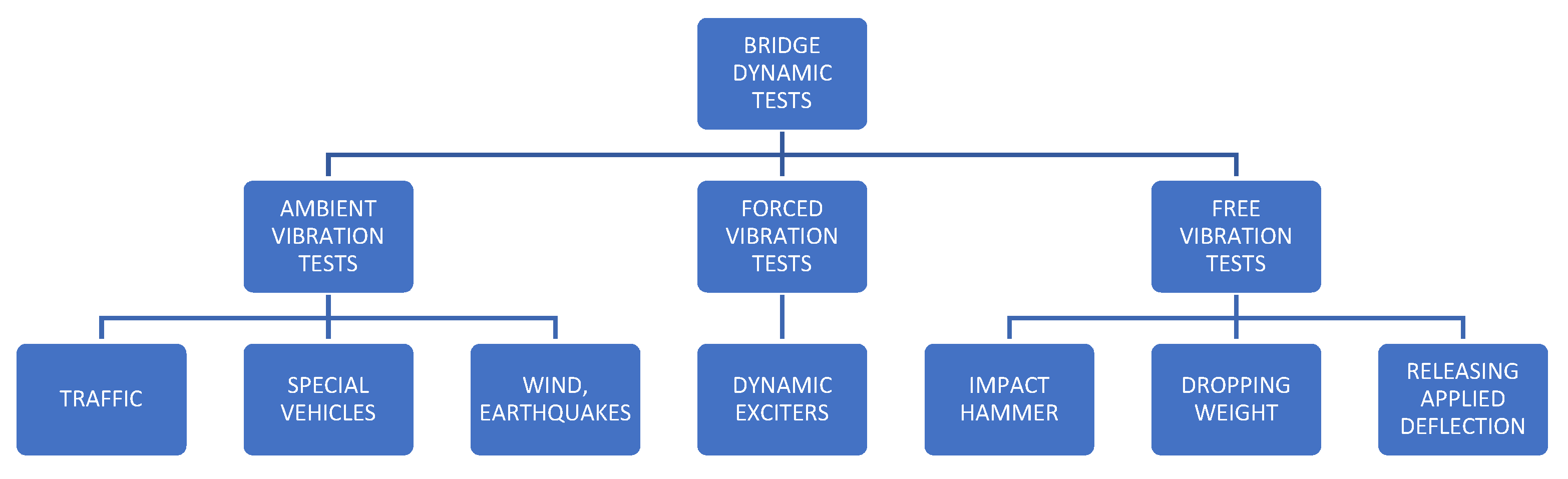
12]. Many testing methods and algorithms in bridge engineering have been borrowed from mechanical engineering where dynamic phenomena and experimental modal analysis were investigated earlier. However, direct use of all these methods for bridge structures encounters many problems related to the more complex nature of bridge materials (concrete, steel, brick, composite material) and structural typologies (beam-like, suspended, stay-cable). The selection of an appropriate testing method can be based on different considerations: (1) structural type and size, (2) available technologies (for example, wired or wireless), (3) strategic importance of the infrastructure, and (4) costs and effective applicability. The last is often more decisive but, nevertheless, it could be overcome by recursive/multiple tests performed in different zones of the bridge. Indeed, such types of tests allow to know the actual dynamic behavior especially in the cases of infrastructures having a prevalent longitudinal development.
Figure 1 shows a simple scheme of the most popular dynamic tests on bridges where, as mentioned before, the ambient vibration ones are surely the most applied.
In the beginning, the experimental identification of relevant dynamic properties of bridges was carried out on the basis of conventional modal testing procedures previously developed in the fields of mechanical and aeronautical engineering. Such tests involved the estimation of a set of Frequency Response Functions (FRFs) relating the applied force and corresponding response at several pairs of points along the structure. These required the use of an articulated instrumentation chain needed for structural excitation, data acquisition, and signal processing. Although forced vibration tests may lead to very accurate modal estimates, they present a strong drawback when dealing with large structures. Indeed, the difficulty in exciting the most significant modes of vibration in a low range of frequencies with sufficient energy is often very demanding in terms of both costs and specialized technical personnel. For example, in the case of small and medium-size structures, the excitation can be induced by an impulse hammer that, thanks to its capacity of providing a wide-band input, is able to excite different modes of vibration. For this reason, the main drawbacks of these types of tests concern the lack of energy to supply the whole experimental layout. Therefore, ambient vibration tests gradually became the most applied, especially for evaluating serviceability conditions or the level of structural rehabilitation [
13,
14,
15,
16,
17].
The results obtained from the application of different output-only modal identification techniques applied to ambient response data collected during two dynamic tests of a cable-stayed bridge and the subsequent finite element model updating are presented in [
18]. The first test, performed by using a traditional data acquisition system with servo-accelerometers, was aimed at investigating the vertical dynamic characteristics of the bridge. In the second test, an innovative radar vibrometer was used for non-contact measurement of deflection time series of the forestays aiming at identification of local natural frequencies of the stay cables. In the numerical analysis, vibration modes were evaluated using a 3D finite element model of the bridge and the information obtained from the field tests, combined with a classic system identification technique, provided a linear elastic model, accurately fitting the modal parameters of the bridge in its actual condition. Another structural typology has been analyzed in [
19]. In this case, the SI has been strongly affected by the mechanical properties of the bearing devices supporting the deck superstructures. Subsequently, the identified features have been compared with those predicted by a preliminary finite element model. This latter has been taken into account as a base line model for monitoring and condition assessment programs related to this infrastructure.
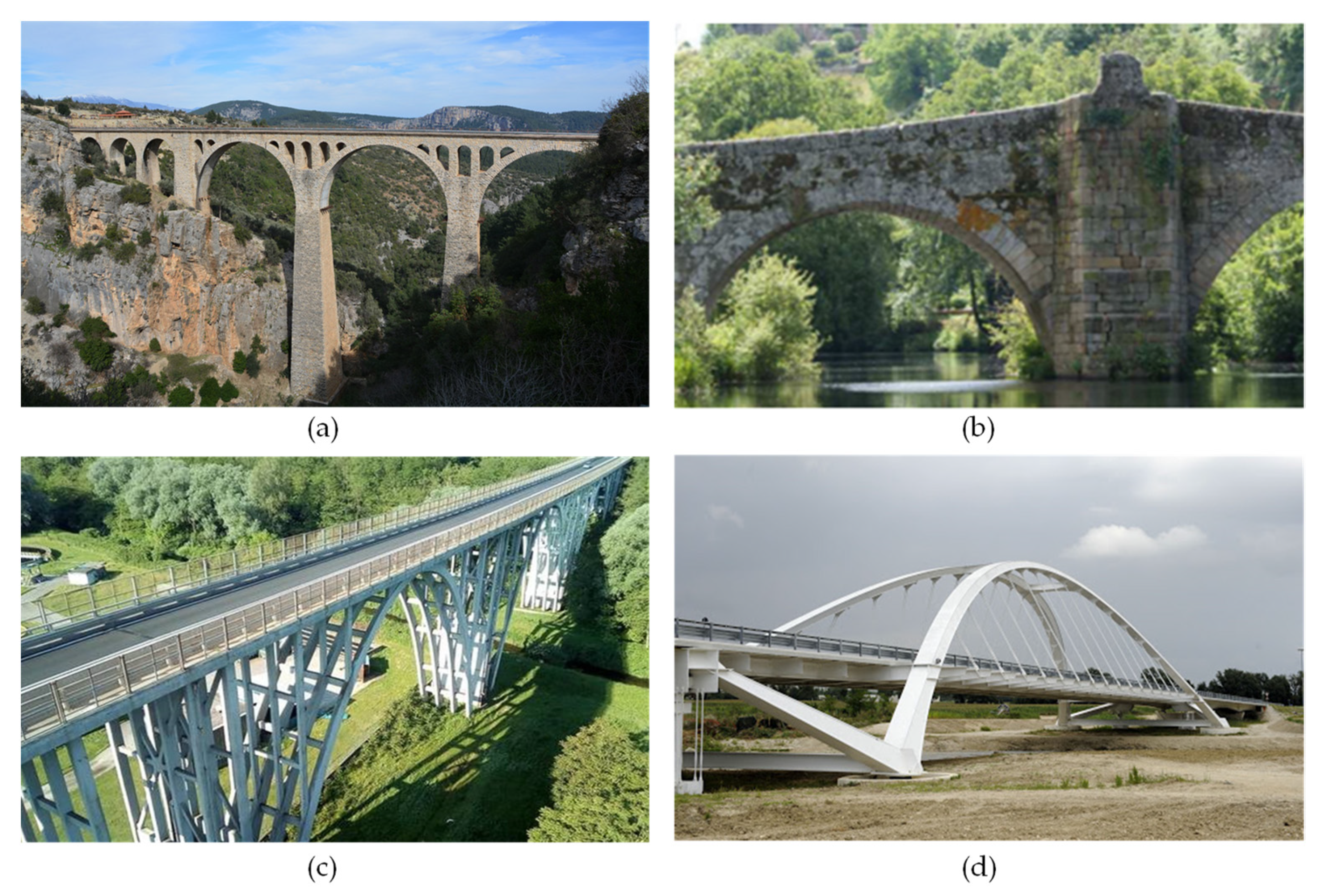
Historically, arch bridges have been mostly known as masonry structures (
Figure 2a,b [
20,
21]) but worldwide examples have been also realized using different materials (
Figure 2c,d [
22,
23]).
In [
20], a model calibration has been pursued based on the information coming from both dynamic and static tests. Afterwards, refined models, representative of the experimental behavior, have been used for structural assessment especially in the verification of the capabilities to withstand train loads. The results of ambient vibration tests applied on reinforced concrete arch bridges have been illustrated in [
22]. In this work, notwithstanding the asymmetry configuration of the viaduct, vertical and lateral modes have been successfully identified processing output-only measurements by two classical procedures such as Peak Picking and Enhanced Frequency Domain Decomposition. An excellent agreement has been found between the two sets. Further, manual model updating has been pursued varying the Young’s moduli of the main concrete components. Recently, ambient vibration tests have been carried out also on modern concrete arch bridges built using both reinforced concrete and steel. An example can be found in [
23], where dynamic tests have been performed with different loading conditions. Even in this case, suitable numerical models have been developed to interpret and represent experimental evidence. In [
24], the results of a huge experimental campaign (845 dynamic load tests) carried out on 11 masonry arch bridges to characterize the vertical and lateral response by different parameters such as train formation and speed, span length, rise/span ratio, and first natural frequencies have been highlighted.
Here, in the illustrated examples the modal identification is based on the processing of a few numbers of experimental tests. A minimum statistical in-depth analysis is carried out only processing the same measurements through different identification procedures. Moreover, as mentioned, a complete investigation of large infrastructures becomes difficult using both wired and wireless equipment. Indeed, in the first case there are problems related to the deployment of electric/communication cables while in the second one it is possible to encounter issues of synchronization. For these reasons, in this work a way to overcome such obstacles will be shown through multiple experimental tests realized in different portions of the infrastructure. The first part will be dedicated to the results of experimental research related to the dynamic behavior of a reinforced concrete multi-span arch bridge. In the second one, critical aspects in the SI and manual model updating of such complex structure will be pointed out. Moreover, the results provided by statistical processing of the information coming from recursive or multiple experimental dynamic tests will be illustrated. The information acquired in the fast experimental campaign furnishes relevant suggestions for the design of a permanent structural health monitoring installation based on vibration measurements.
2. Dynamic Tests on the Case Study
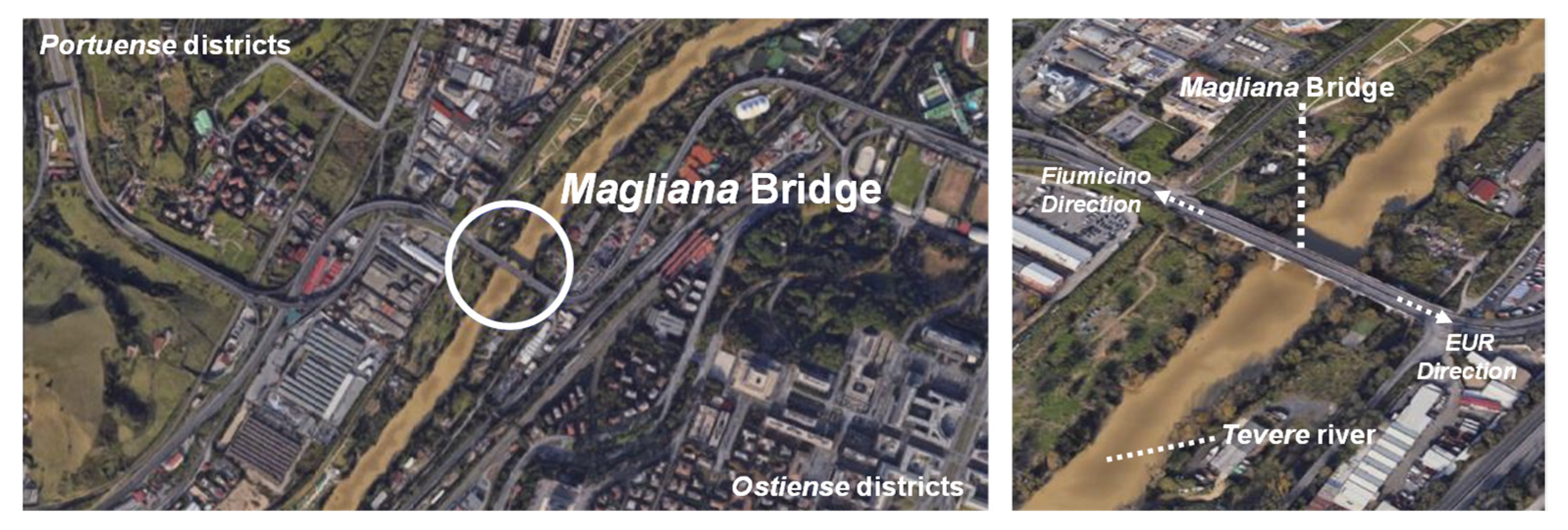
Since the dawn of time, the city of Rome has been crossed by the “
Tevere” river. Thanks to its presence, a wide number of bridges were constructed to cross the same river. In this context, one of these bridges is the subject matter of this research and it is called “
Ponte della Magliana”. An overview and zoomed-in view from above of its location are reported in
Figure 3.
The bridge connects the “Portuense” and “Ostiense” districts of Rome, respectively, located in northwest and southeast directions with respect to the river. It was designed in 1930 and built to be the entrance to the western side of the new “EUR” district. Its complete realization was only after the second world war. It is currently part of a larger highway that, in the west direction, continues towards the “Portuensi” hills and the highway to “Fiumicino” airport while on the east it leads towards the “EUR”, “Tre Fontane”, and “Laurentina” districts.
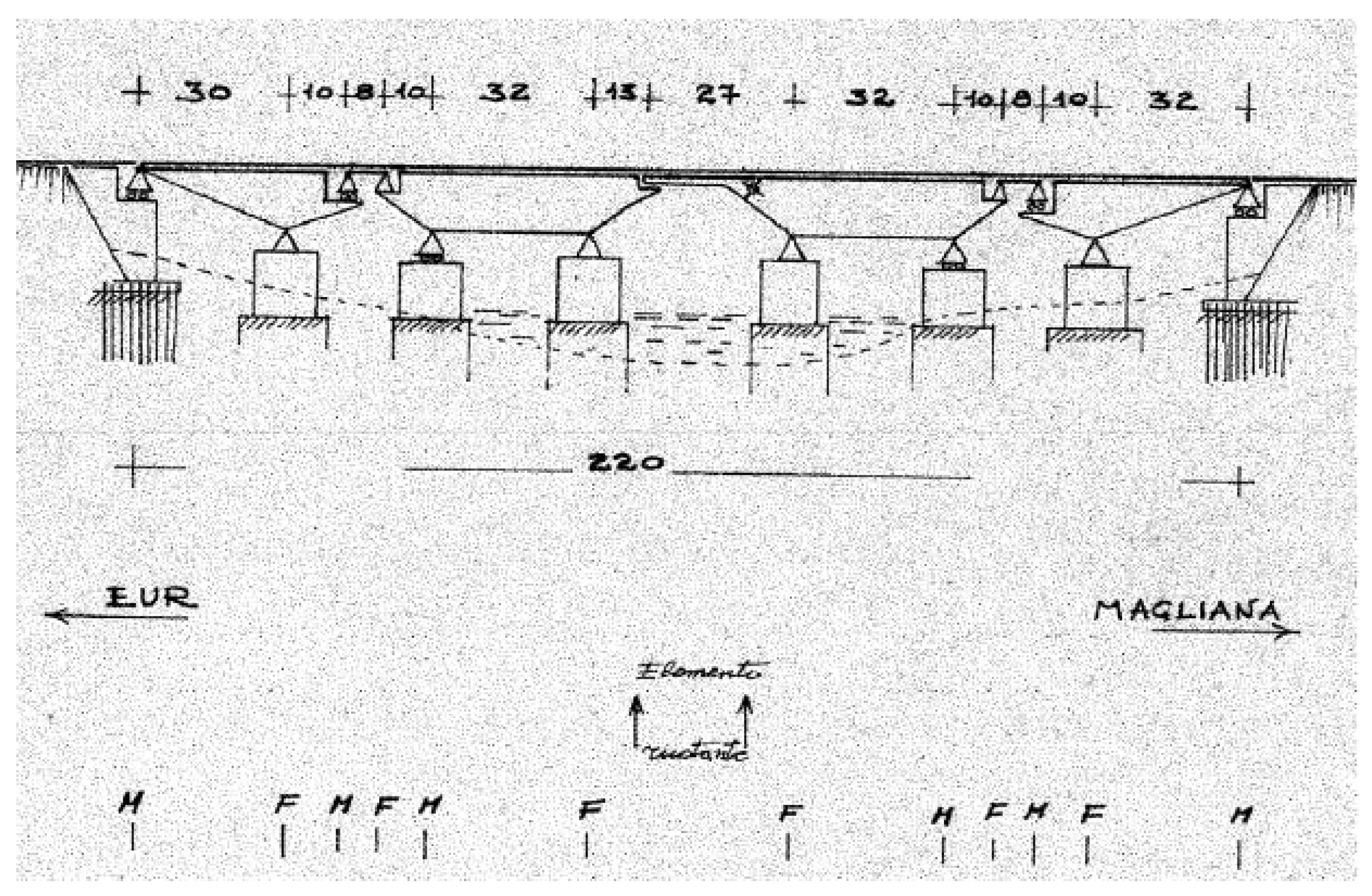
The structure is a reinforced concrete arch bridge, with a length of about 225 m. It develops linearly through 7 spans and rests on 2 abutments and 5 piers, 2 of which are in the riverbed and 4 outside the riverbed. The length of each span is about 30 m except for the central and moveable span that presents a length of about 40 m. The static scheme is a supported beam, as shown by the original drawings preserved by the municipal technical office [
25] and illustrated in
Figure 4. Such configuration aimed to minimize the internal stresses due to possible failures related to the supports of the isostatic system.
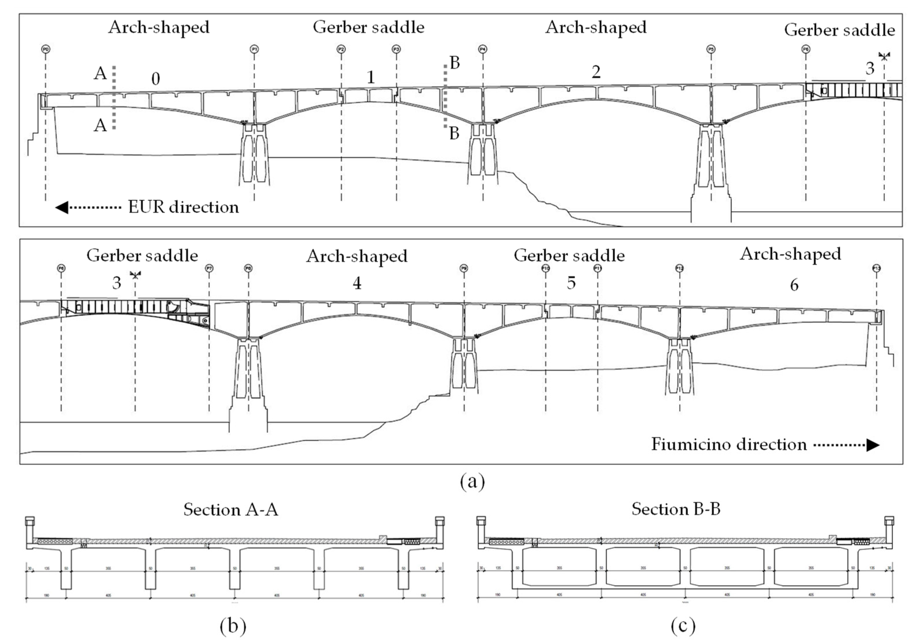
This static scheme divides the bridge into four isostatic substructures that are capable of absorbing possible structural failures (e.g., subsidence) without generating states of internal compulsion. Such scheme allows the structure to remain in the elastic field following small altimetric and planimetric variations of piers and abutments and so, for this reason, is particularly suitable for river crossings. The fundamental structural element that allows such configuration is the Gerber saddle that represents a peculiarity of this bridge. As visible in
Figure 5a, the overall composition shows four arch-shaped spans linked together by three Gerber saddles. The concrete decks have a multi-box section, separated by five septa with a thickness of 0.50 m. Since each span presents a longitudinal curvature, the height of such transversal section is variable along the span length with a maximum and minimum value corresponding to the supports and central line, respectively. On the extrados of the section, there is a concrete slab, with an average thickness of 0.20 m, while in the intrados there is a slab showing a variable thickness only in particular zones of the bridge.
The steel deck (that was previously moveable) has a static layout of a supported beam. The main beams are made up of pairs of double T beams variable in height and thickness. Between such two beams, double T sections are positioned transversely. The extrados slab, in reinforced concrete and connected by pegs to the steel beams, is 0.20 m thick and rests on UPN200 steel profiles. In
Figure 5b,c, two examples of transversal sections are reported with an open profile and multi-connected, respectively.
2.1. Experimental Layouts
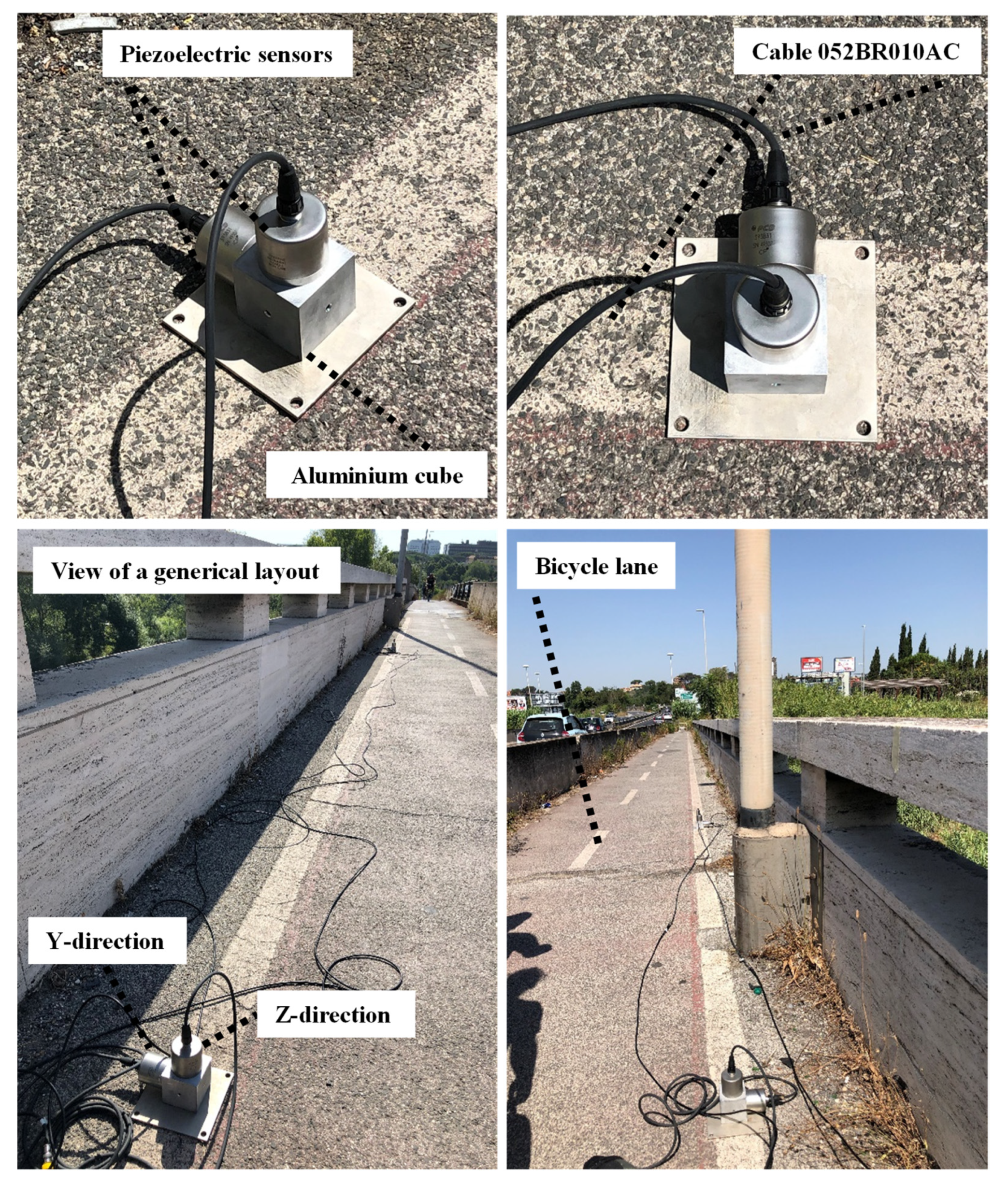
The dynamic tests were carried out in a one-day experimental campaign through which accelerometric measurements were recorded. The tests were implemented during a very sunny day (30 July 2020) and the traffic conditions were very intense. Ambient vibration tests were conducted on the five central spans of the bridge using a 12-channel data acquisition system, LMS SCADAS XS, with n.6 piezoelectric uniaxial accelerometers, PCB model 393B31, and a Smart Scope.
LMS SCADAS XS constitutes the main part of the data acquisition system and, thanks to its manageability, it is very suitable to optimize the implementation of the dynamic tests. It is very useful for carrying out both real and reduced-scale tests. The main characteristics to be underlined are the following:
The board has a very small dimension (as a tablet pc) and, moreover, it has a built-in battery.
It can have three different modes of operation: Wi-Fi (connected to Smart Scope), stand-alone, and front-end.
It can support 12 analog channels.
The Smart Scope is a tablet on which the user can set up, control, and manage the measurement template and carry out online data processing. The most relevant parameters to be set up are sensor name, point ID and point direction, typology of the physical quantity to be recorded and its unit of measure, sensitivity, and acquisition sample rate. The piezoelectric accelerometers, employed in the dynamic tests, are PCB 393B31 realized with ICP technology that requires only an inexpensive, constant-current signal conditioner to operate. Their main features are illustrated in the following
Table 1.
The link between the sensors and acquisition system is completed by a complementary instrumentation. This latter is composed of different typologies of coaxial cables used for both transmissions of the measured data and power supply. In particular, two cables (coaxial cable RG 178/179 and custom cable 052BR010AC), from a side, have to be linked to the board LMS SCADAS and to the piezoelectric sensor, respectively, while the third cable (coaxial cable RG58) must be linked in the other free end of the two previous cables (it only has an extension function).
Moreover, in order to realize a reliable link between the sensor and structure, a customized aluminum cube with a central thread for screw insertion was realized, in each face, needed for the connection of the accelerometric sensor. Furthermore, in one of the six cube faces, four magnetic elements were introduced for a rapid and easy connection in steel or iron structure points. In the photos reported in
Figure 6, the presence of a bicycle lane is visible, located in both external lines of the bridge, that allowed an easy implementation and execution of the dynamic tests.
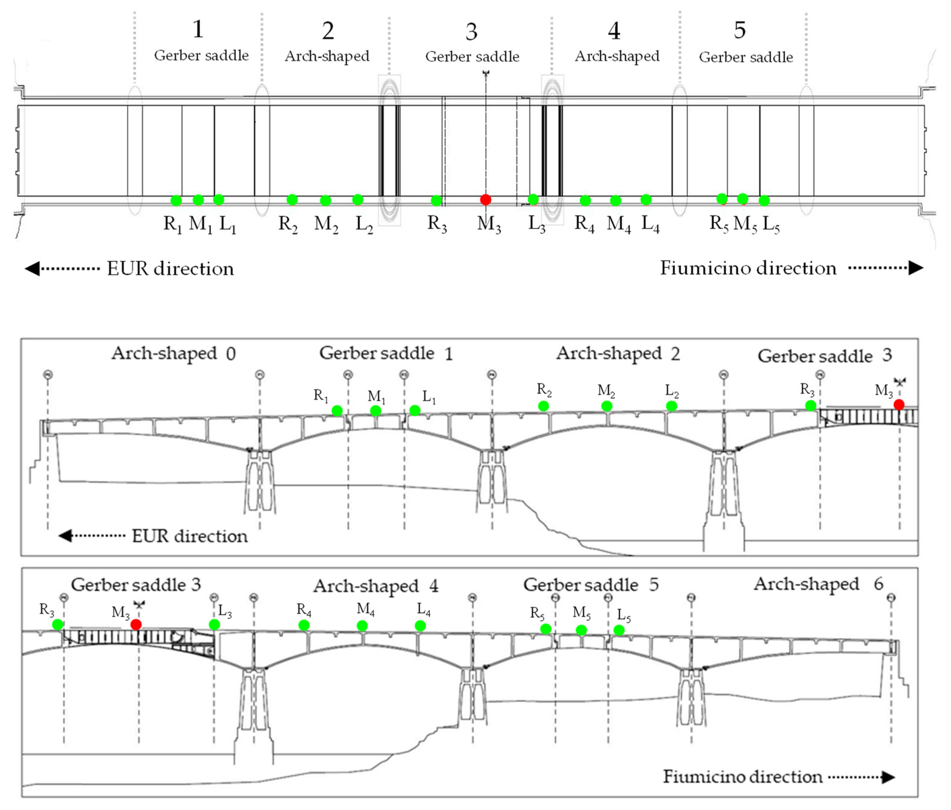
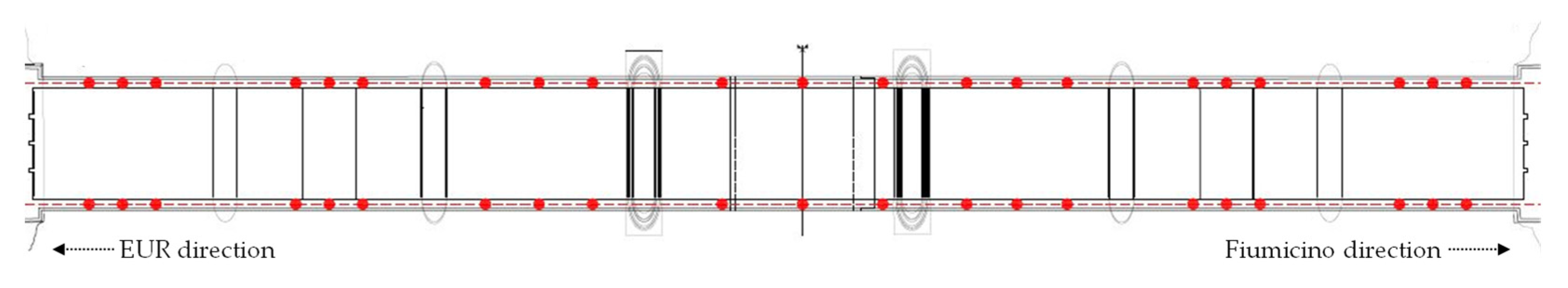
The five spans, the object of the dynamic tests, are indicated in
Figure 7 where, moreover, a well-defined code was assigned at each sensor position for an unequivocal identification. In each position (highlighted by green circles in
Figure 7), two piezoelectric uniaxial accelerometers were installed in a biaxial configuration in order to identify the dynamic behavior of the following directions:
Three sensor positions were designed for each span. One position is always located in the middle of the span length and so, in the case of the Gerber saddle span, it is in the middle of the corresponding saddle. The other two positions were selected on the right and left with respect to the middle with the aim to also identify anti-symmetric modes. Moreover, in each position, two PCB accelerometers were installed: in the Z- and Y-directions, respectively. For each position, the following identification parameters were assigned:
Position on the span: R: right; M: midpoint; L: left.
Number of the span: 1, 2, 3, 4, and 5.
Direction of the measurement: Z, Y.
The whole time of acquisition was not the same for each span. In particular, 1800 s was adopted for the span n° 3 while 1200 s for the other spans. The sample frequency for data acquisition was 200 Hz for all tests. Spans n° 1 and n° 5 are characterized by the presence of two Gerber saddles (one for each span) realized by a simply supported deck that divides the corresponding span into three elements. In order to study the different structural response of the three elements, one accelerometer was set on the midpoint deck and the other two were positioned externally to the saddle. Spans n° 2 and n° 4, differently from spans n° 1 and n° 5, did not have Gerber saddles but an arched profile. In this case, one accelerometer was set on the midpoint and the other two were located at a certain distance from the midpoint one. A particular configuration can be observed in the case of span n° 3. Indeed, it shows a central steel saddle Gerber. Originally, this latter was a removable steel element span but, over time, it was modified and fixed. Moreover, this element presents on one end (side EUR direction, left in the
Figure 7) a simple constraint (like a roller), while in the other one it is rigidly connected to two cantilever steel beams. Additionally, in this case, one position was set on the midpoint and the other two at a certain distance from such midpoint. Regarding the two sensors located in the midpoint, unfortunately, for technical and safety reasons, it was impossible to realize a reliable connection to the structure; therefore, their recorded accelerations were not considered in the subsequent processing (this position is highlighted with a red circle in
Figure 7).
2.2. Modal Identification: General Background
One of the more traditional approaches applied to estimate the modal parameters of a structure is the Peak Picking (PP) method [
26]. Such method could lead to reliable results if, as basic assumptions, the modes to be identified have low damping and are well-separated from each other. In fact, when a lightly damped structure is subjected to a random excitation, the output auto-spectral densities at any response point will reach a maximum at frequencies related to the modal signatures of the structures. Since narrow-band peaks in the frequency response function of lightly damped mechanical systems occur at the frequencies corresponding to normal system modes (resonance frequencies), peaks in the auto-spectral densities and cross-spectral densities can be generally assumed to represent the normal modes of the structure.
An evolution of the PP method is the Frequency Domani Decomposition (FDD). This technique involves the following main steps:
Estimate of the spectral matrix.
Singular Value Decomposition (SVD) [
27] of the spectral matrix at each frequency.
Inspection of the curves representing the singular values to identify the resonant frequencies and estimate the corresponding modal shape using the information contained in the singular vectors of the SVD.
FDD is a rather simple procedure and represents a significant improvement in the PP since:
SVD is an effective method to analyze, in depth, the spectral matrix characteristics and the evaluation of the mode shapes is automatic and significantly easier than in the PP.
The FDD technique is able to detect closely spaced modes. In such instances, more than a singular value will reach a maximum in the neighborhoods of a given frequency and every singular vector, corresponding to a non-zero singular value, is a mode shape estimate.
Damping ratios can be identified through a refinement of the FDD technique, called Enhanced Frequency Domain Decomposition (EFDD).
The EFDD technique is based on the fact that the first singular value in the neighborhoods of a resonant peak is the auto-spectral density of a modal coordinate. Hence, taking back the partially identified auto-spectral density of the modal coordinate in the time domain, by inverse fast Fourier transform, a free decay time domain function is obtained. This latter represents the autocorrelation function of the modal coordinate. The natural frequencies and the related damping ratios are thus simply found using the peak of the auto-spectral densities and logarithmic decrements, respectively.
2.3. Modal Identification: Case Study
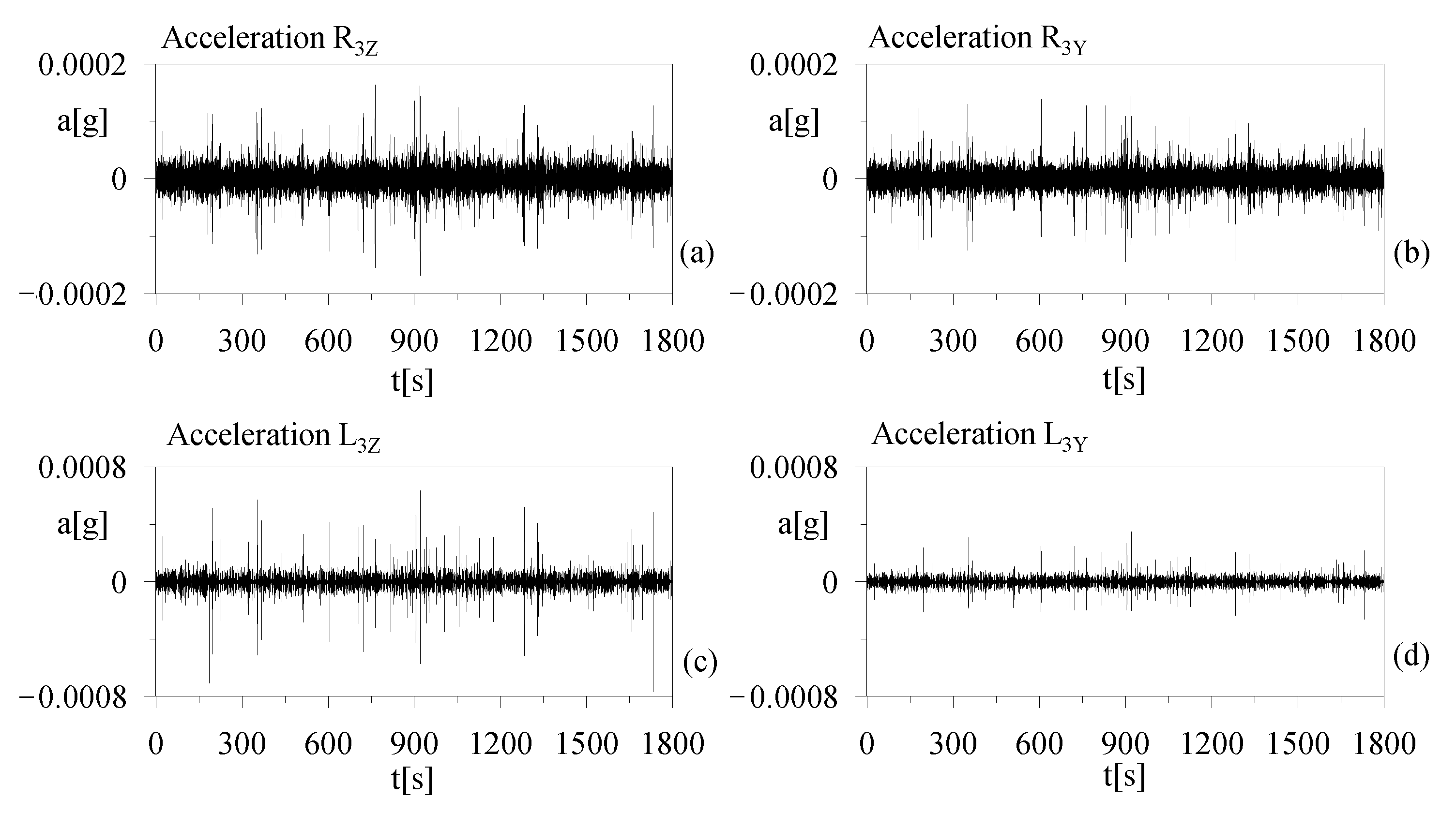
The identification of modal parameters was developed using two different output-only procedures: the Peak Picking (PP) and the Enhanced Frequency Domain Decomposition (EFDD). The EFDD procedure is a refinement of the Frequency Domain Decomposition technique. Both the PP and FDD/EFDD methods are based on the evaluation of the spectral matrix (i.e., the matrix of cross-spectral densities) in the frequency domain. In
Figure 8, some examples of the acquired acceleration during the tests are reported. In particular, they were recorded by the experimental layout installed in span 3.
It can be observed that the accelerations related to the sensors of the right position (
Figure 8a,b) show a lower amplitude with respect to the left ones (
Figure 8c,d). Additionally, the corresponding standard deviations (σ) show low values: σ
R3Z = 1.1286 × 10
−5 g, σ
R3Y = 9.7175 × 10
−6 g, σ
L3Z = 1.8621 × 10
−5 g, and σ
L3Y = 9.6748 × 10
−6 g. They are lower in the right position and in general the transversal direction (Y) is harder to excite. Moreover, a wide presence of spikes due to the passage of trucks of large dimension are clearly visible.
For the case studied, the modal identification was performed through a procedure implemented in Matlab software found in the literature [
28]. First of all, the accelerometric signals were subjected to a lowpass filter with a frequency range between 0 and 20 Hz. The Power Spectral Densities (PSDs) were obtained with the periodogram function while mode shapes with the Automated Frequency Domain Decomposition (AFDD) function [
28]. In
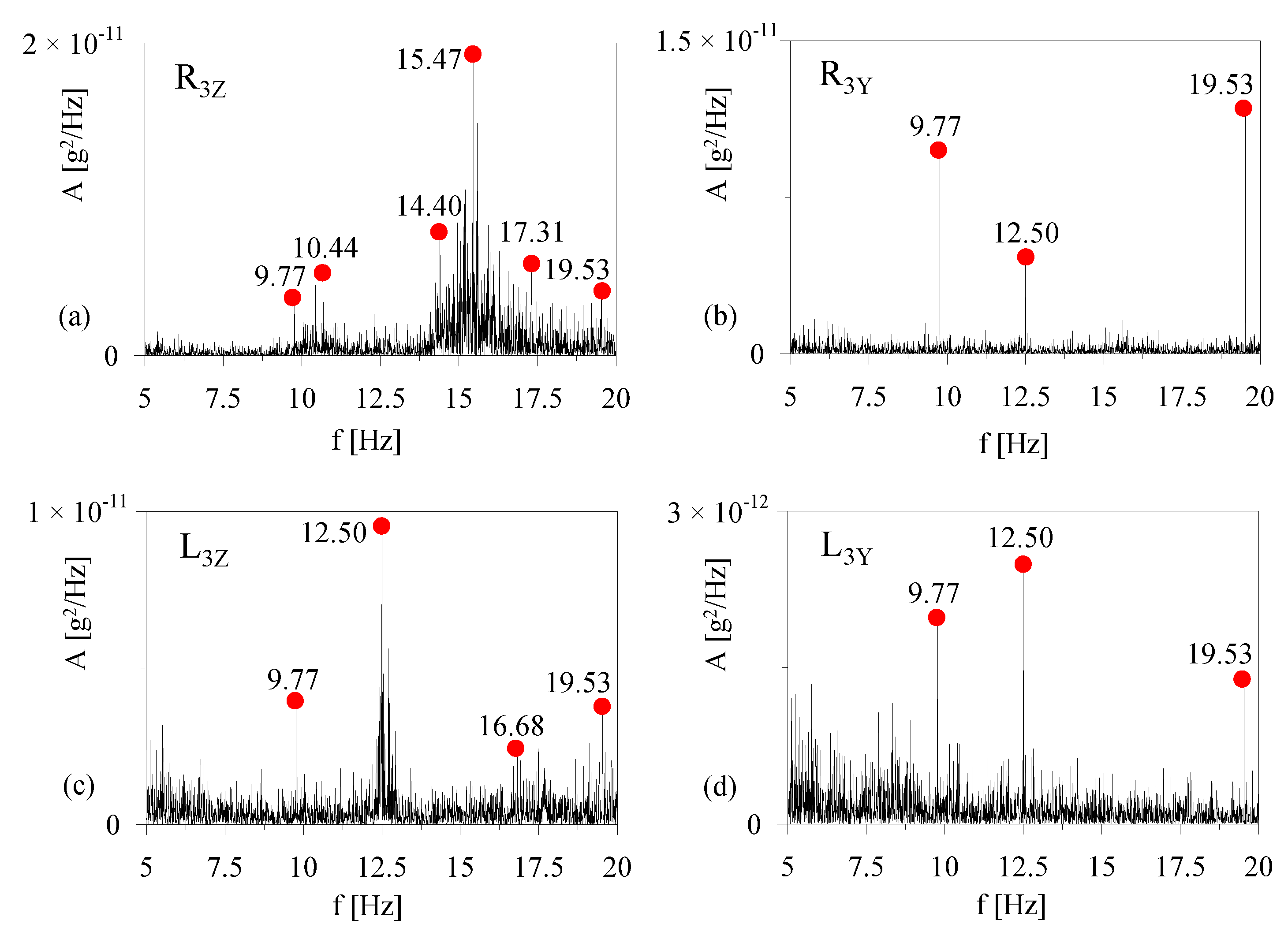
Figure 9 the PSDs in Y and Z directions calculated by processing the measurements obtained during the test on the span n° 3 are shown. Looking at the results provided by such PSDs, it is possible to observe that in the Z-direction, well-defined peak values corresponding to the structural modes are difficult to recognize (
Figure 9a,c). Instead, in the Y-direction peak values are clear and easily identifiable (
Figure 9b,d). By comparing the results found in the PSDs calculated for both directions, the frequencies reasonably associated to the structural modes were identified. They are reported in the following
Table 2.
Due to the fact that in the Z-direction it is hard to define peak values (this is also a consequence of the very small amplitude measured), a probabilistic approach was implemented on all values (in all five tests) obtained in both directions for a more robust identification. The probabilistic approach was organized based on the following three phases:
Identification of the presumable frequencies coming from the measurements obtained in the five dynamic tests carried out (in total 28 accelerations recorded, 14 in each direction Y and Z).
Identification of the frequencies with the highest number of appearances.
Graphical representation with a bar histogram for a better visualization.
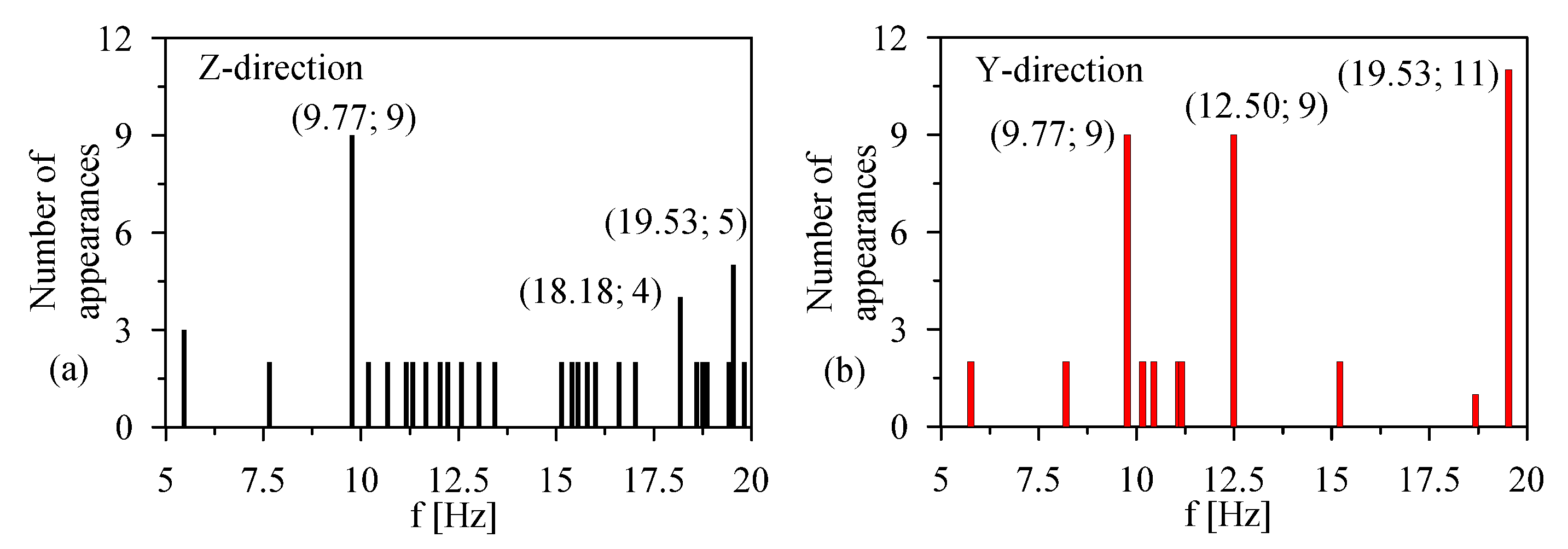
The results of the probabilistic approach are illustrated in
Figure 10. In such graphs, the frequencies most detected by analyzing the accelerations recorded in both Z- (
Figure 10a) and Y- (
Figure 10b) directions in all dynamic tests are reported. Substantially, the two frequencies mostly found in both directions are 9.77 and 19.53 Hz. Two other frequencies, 18.18 Hz only in the Z-direction and 12.50 Hz only in the Y-direction, appear more frequently than others. The latter one could be more reliable since it has been found more times with respect to the first one. The final set of the identified frequencies is shown in
Table 3.
Regarding the experimental layout, due to the presence of intensive traffic it was not possible to implement a configuration in the center longitudinal line of the roadway. Of course, if such measurements were recorded they would have helped in the correct identification of the coupled modes.
With the aim to deepen the statistical analysis, in
Table 4 and
Table 5 the number of appearances of the first three identified frequencies with varying numbers of the experimental tests are reported. In particular, in
Table 4 the trend for the modes in the Z-direction is illustrated while in
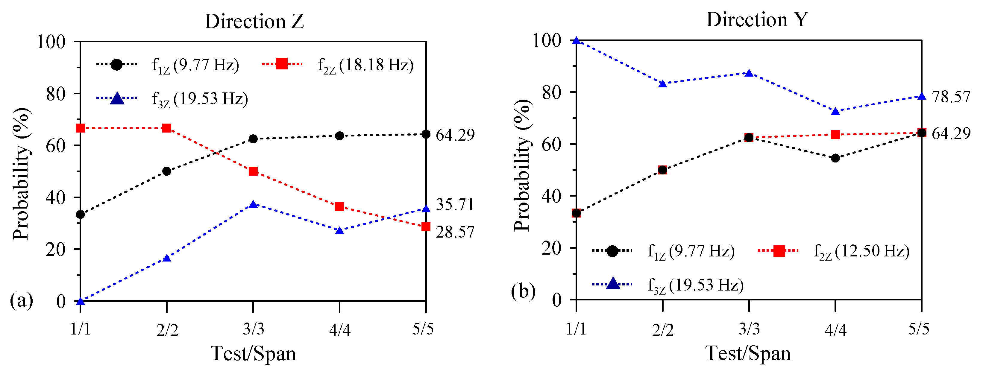
Table 5 for those in the Y-direction. It is evident that such frequencies are not always identifiable for different motivation: (1) they could be referred to local modes, (2) in correspondence with a zero-modal coordinate, or (3) due to a very low amplitude (that means a very low signal/noise ratio). For these reasons, in
Figure 11 the dependence of the probability of appearance with varying numbers the tests is shown. Some observations are the following:
The modes corresponding to the frequencies 9.77 Hz (in both directions) and 12.50 Hz appear in almost all PSDs showing the same final probability of 64.29%. They could be associated to global modes.
A little doubt could be raised by the mode at 19.53 Hz. Indeed, such frequency is not always visible in the Z-direction (35.71%) but, regardless, it is commonly found in the Y-direction (78.57%).
The mode at 18.18 Hz is the most difficult to understand. Substantially, it is visible only in the Z-direction for the first two spans (28.57%). Some other suggestions could be provided by looking at the modes of the numerical model.
To complete the identification process, even if in an approximative way, the damping ratios in correspondence with the experimental modes are reported in the following
Table 6.
3. Finite Element Modeling
The bridge was modeled through a numerical finite element model implemented in MIDAS Civil software. The whole model is composed of 548 nodes and 1129 elements (740 beams and 389 plates). The deck of the spans 1, 2, 4, and 5 is made of concrete, for which a class C20/25 was adopted (specific weight of 25 KN/m
3) with Young’s modulus assumed equal to 29.96 GPa. Instead, span n° 3 has a steel deck and so a steel class of S275 (specific weight of 76.98 KN/m
3) with Young’s modulus of 210 GPa was assumed. All constitutive models selected were elastic and linear. The initial parameters were selected based on the information found in the original design documents. The density of the mesh is variable along the structure. For plate elements, on average, there is an element at each 14 m
2 but near the supports and over the steel central deck a refinement of 6.5 m
2 and 3.5 m
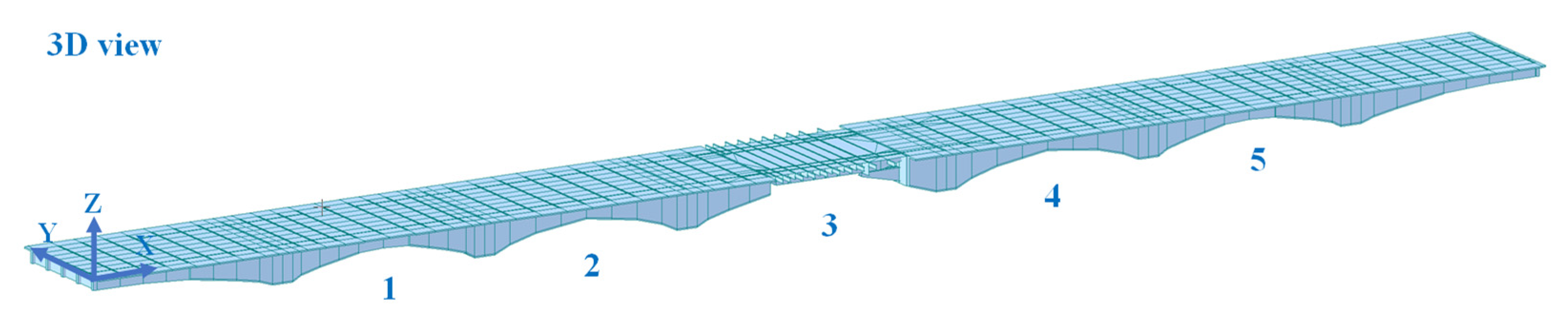
2, respectively, was carried out. In
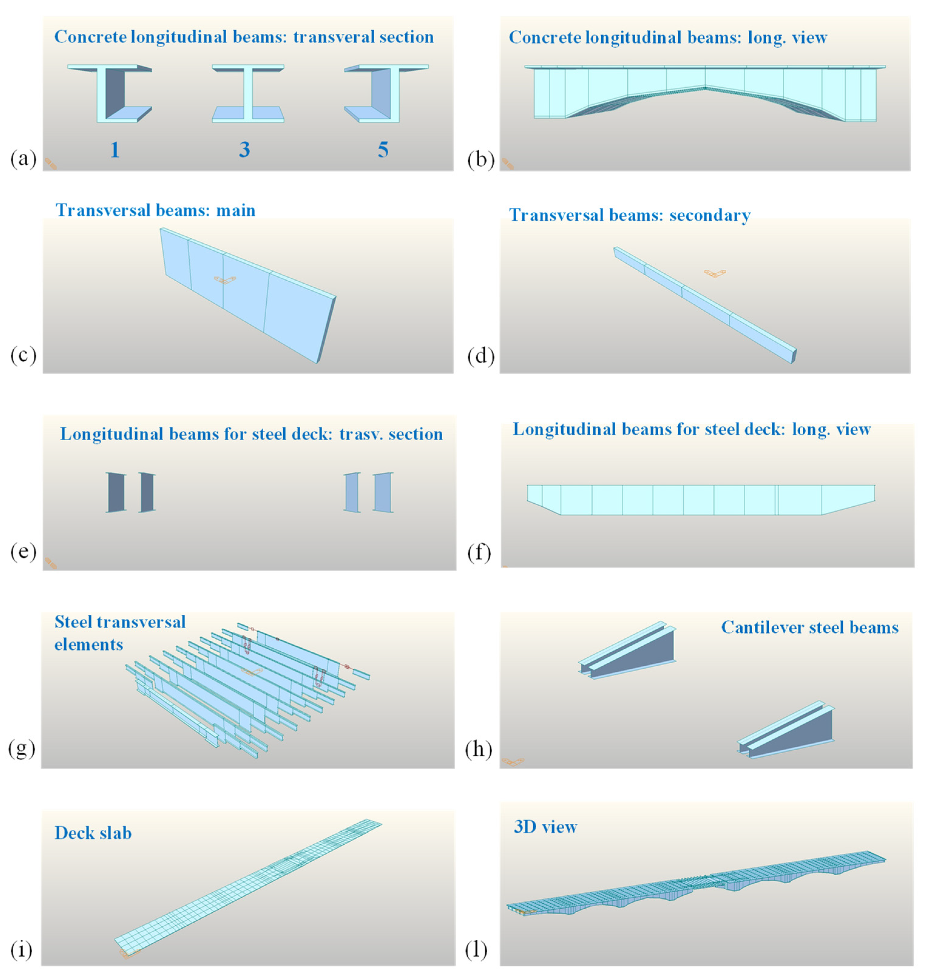
Figure 12 the 3D view of the implemented model is illustrated.
The principal elements of the model are the following:
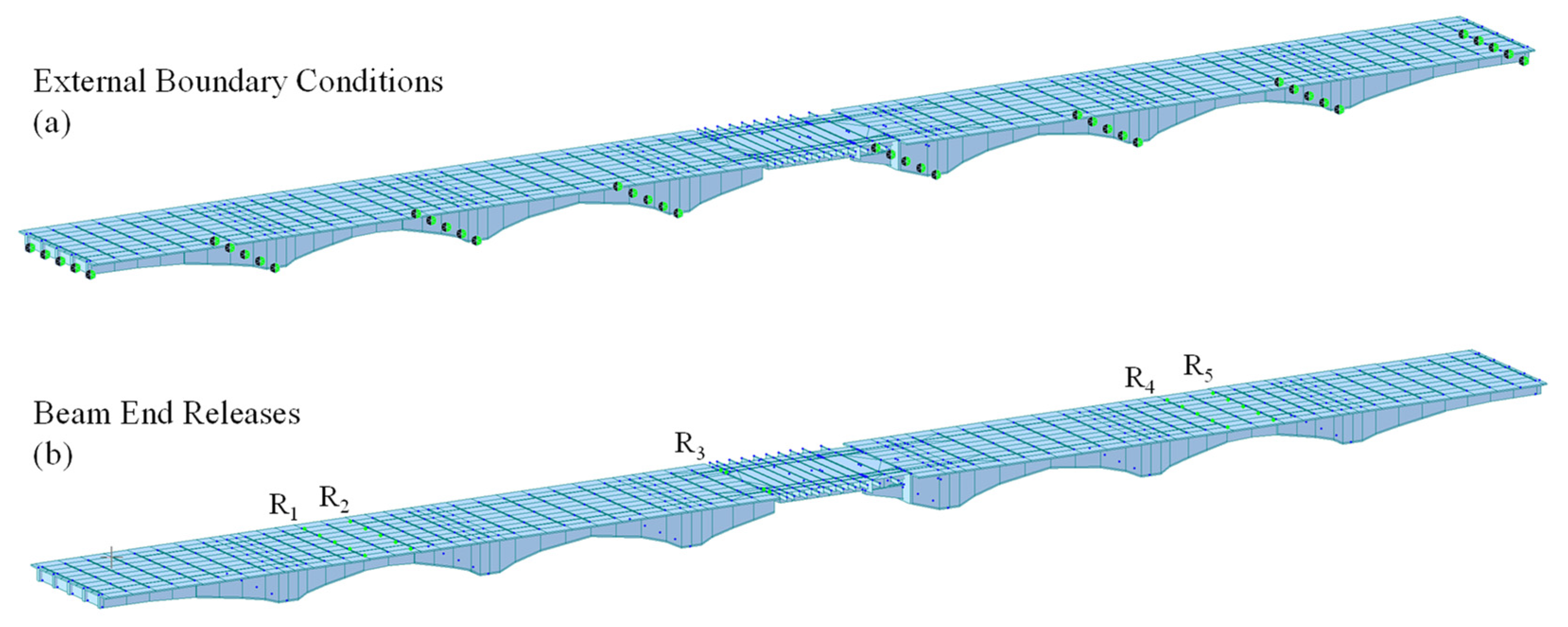
The boundary conditions for the model are divided into external and internal (end releases) ones in
Figure 14a,b. The first are restraints that connect the deck with the substructures (piles and lateral abutments). The end releases were applied in the corresponding Gabble saddles (R
1–R
5 in
Figure 14b). In particular, in each node, contained in correspondence with the transversal lines R
1–R
5 removed the bending moments and longitudinal normal forces as indicated in
Table 7. Both external boundaries conditions and beam end releases were modeled consistently with what was reported in the original static sketch. Moreover, to better represent the structural behavior of the bridge, a rigid plan constraint was introduced through the function rigid link. All the nodes of the model were connected with a rigid link to a master node, positioned in the center of the whole bridge. To complete the model implementation, the road pavement was taken into account using a uniformly distributed load of 2 kN/m
2 acting on the elements representative of the deck slab. The numerical modal analysis was subsequently carried out and the results in terms of frequencies, participating mass, and modal shapes are reported in the following
Table 8 and
Figure 15.
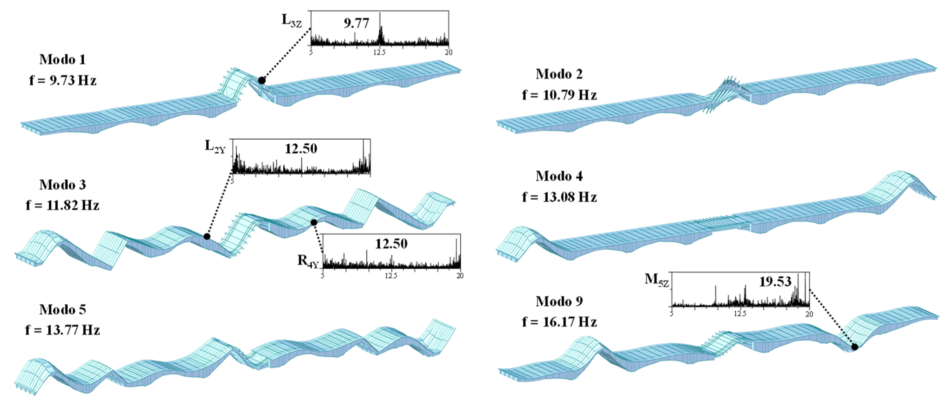
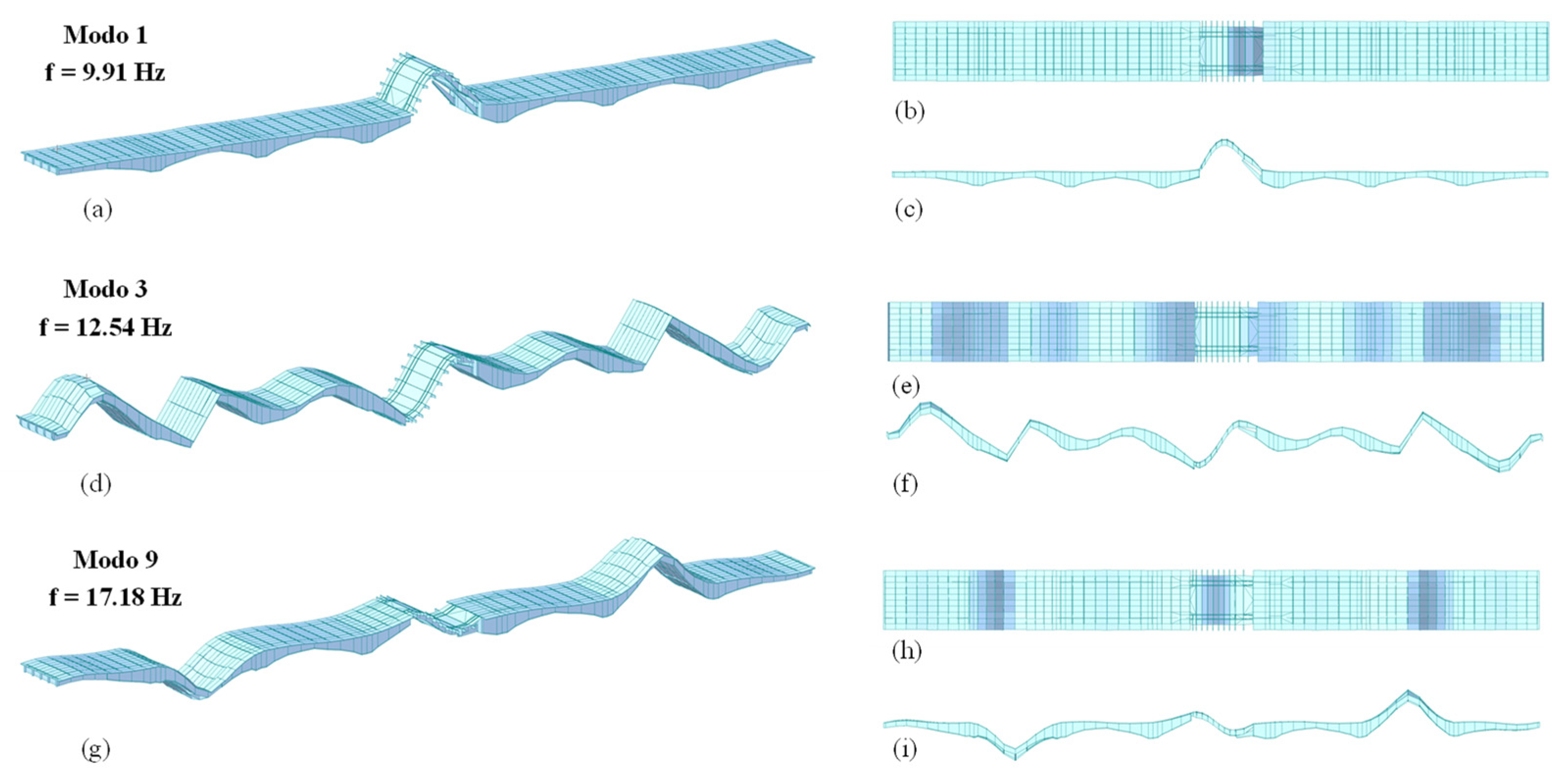
The results of the numerical modal analysis related to an initial model defined using nominal parameters (as, for example, the elastic modulus; in the following such initial model will be called the
nominal model) are reported in
Table 8. In particular, in grey the main modes in Z- and Y-directions, very close to the identified ones, are highlighted. Mode 1 shows a bending deformed in correspondence with the central Gerber saddle (span 3) and, moreover, its frequency (9.73 Hz) is very close to the first identified mode. The same observation can be made for the third mode (11.82 Hz) that, moreover, exhibits a global shape. It could be reasonably associated to the second identified mode (12.50 Hz). Instead, to find a mode close to the third identified mode (19.53 Hz), in both frequency and shape, selection of the numerical mode 9 (16.17 Hz) is required. Mode 2 shows a local and torsional deformed in the span 3. In this situation, the corresponding frequency was not identified since the central measurements in that span (see position M3 in
Figure 7) were not recorded correctly. Instead, mode 4 shows modal displacements in spans 0 and 6 where measurements were not acquired. Mode 5 is a global mode of higher order that was not identified. In
Figure 15 some PSDs that have frequencies associable to the corresponding numerical modes are reported.
Manual Model Calibration
Once the numerical modal frequencies are obtained by the nominal model, a comparison with experimentally identified frequencies is opportune. The target is to make as close as possible the difference between numerical frequencies and identified ones. Such objective was pursued with manual model updates. It is important to focus the attention on the numerical modal frequencies. The three frequencies that were taken into account in the procedure are reported in
Table 9 where a first comparison with the numerical frequencies coming from the nominal model is reported. The percentage difference was evaluated through the following expression:
According to the results reported in
Table 9, the first numerical mode, in the Z-direction, shows good agreement with the experimental one while the third one and especially the ninth have a greater difference. The average difference is 7.68%.
Since the comparison between the numerical model and experimental result frequencies reveals relevant differences for the second and third modes (modes 3 and 9 at 11.83 and 16.58 Hz, respectively), as shown in
Table 9, the numerical model should be optimized in order to minimize these differences.
Analyzing such frequencies, it is possible to observe that experimentally identified frequencies show higher values than numerical ones. The real structure appears stiffer that the numerical one. In order to make the difference between the experimental and numerical modal frequencies as small as possible, a stiffening of the numerical model is pursued by increasing the Elastic Modulus (E) of the concrete. The optimization criterion is driven using the following Objective Function (OF): minimizing the sum of the differences, in absolute value, of the three frequencies associated to the modes selected in
Table 9.
It is correct to underline that in Equation (2) the
OF depends on the
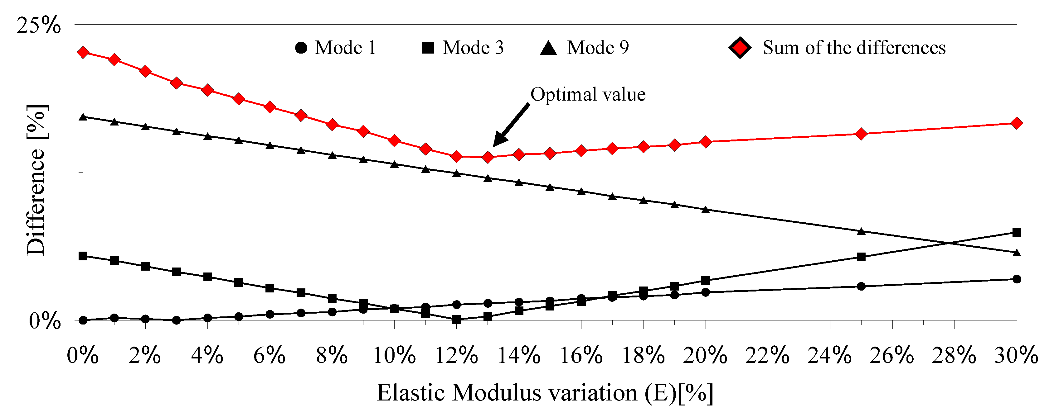
E parameter. In
Figure 16 a parametric analysis of the frequencies altering the Elastic Modulus is reported. This latter is increased within a range of 30% with respect to its nominal value (29,961 MPa), as well visible in the abscissa. In the ordinate, according to Equation (1), the percentage differences between numerical and experimental results are reported. The first (mode 1) and third (mode 9) frequencies undergo an increase and decrease, respectively. Instead, the second one (mode 2) highlights a minimum point corresponding to 13%. The red curve illustrates, instead, the sum of such differences. The results indicate that the optimum value of
E is found increasing its nominal value up to 13%. Therefore, the final value inserted in the updated model is equal to 33,856 MPa. Such value could be considered reasonable since, in general,
E increases over time up to an asymptotic value.
In
Table 10 a comparison between the performance obtained by the initial (nominal) and updated model is reported. Modes 3 and 9, in the updated model, were considerably improved versus a slight detriment of the first mode. Consequently, the OF shifts from a value of 23.05% to 10.28%.
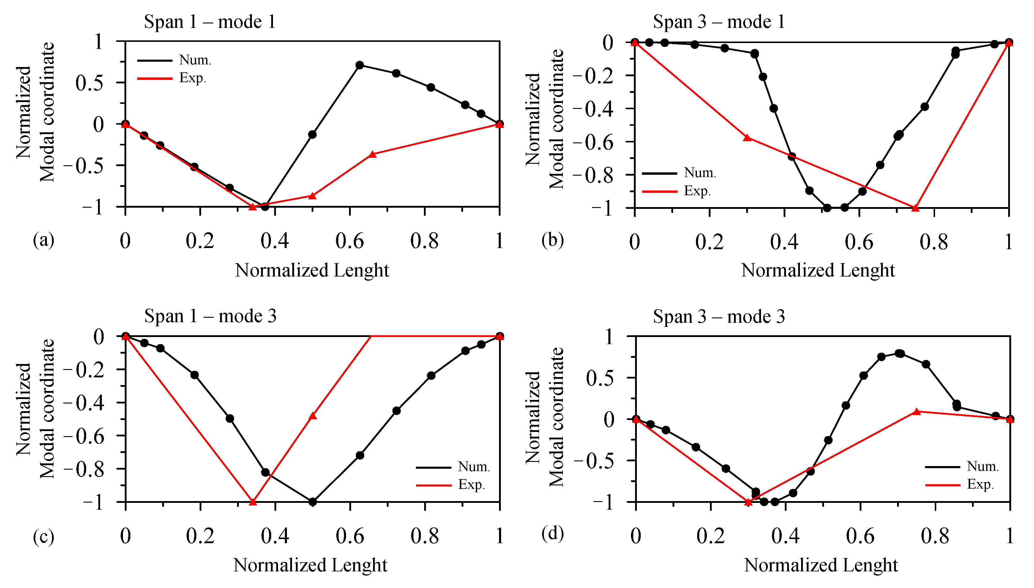
In order to complete the updated process, a comparison between experimental and numerical shapes was also performed. The modal shapes (experimentally identified and numerical) are reported in the Z-direction for modes 1 and 3 in the corresponding spans 1 and 3 in
Figure 17.
Notwithstanding the small number experimental modal coordinates (3 in span 1 and 2 in span 3), a good agreement is clearly visible especially for mode 3 in span 3 where a counterphase behavior is recognizable in L
3Z and R
3Z. Even if it not clearly visible, a slight deformation is shown for span 1, mode 1. In this last case, the counterphase is missing especially due to the low number of measurements. The experimental modal shapes were obtained through the AFDD procedure in Matlab. Finally, in
Figure 18 the modal shapes related to the modes 1, 3, and 9 of the updated model were inserted. It is right to highlight that, after the model updating procedure, such modal shapes are not changed.
4. Discussion
The tests on the bridge were performed in a one-day campaign and they highlighted some difficulties. One is related to maintenance of the bridge in its operational condition, during the tests, guaranteeing the proper flow of traffic. The presence of the traffic if, from the side, made the installation of the experimental layouts difficult; on the other side, it allowed to record accelerations with an adequate amplitude level. Moreover, the intensive traffic did not make the realization of all useful configurations possible due to, for example, the positioning of the sensors in the longitudinal center line of the roadway. Of course, the tests were performed very quickly reducing the typical risks related to the execution of the dynamic tests. A first general suggestion for the execution of vibrational experimental tests on bridges is the following: the use of wired instrumentation raised issues due to the deployment of the communication cables and so, especially for the experimental activity on bridges or viaducts, a wireless sensor nodes network is advisable. However, in the last case, an opportune choice of the Micro Electro-Mechanical System (MEMS) sensor, with sufficient sensitivity, is needed. The results from the use of recursive/multiple tests suggest that, especially for bridges showing a very long longitudinal configuration, they could provide useful indications. Indeed, a statistical approach helps with removal of possible uncertainness related to few measurements available and the complexity of the structure.
It was also found that the peaks in the acquired time histories were due to the passage of heavy vehicles on the bridge. This observation suggests that the number of times in which the accelerations overcome a well-defined threshold is equivalent to the same number of heavy vehicles transiting. In old bridges, as in the case study analyzed in this paper, it could be important to know statistical information related to the passage of particular typologies of vehicles and monitor the evolution over time.
Therefore, the installation of a vibration-based Structural Health Monitoring (SHM) system would allow the acquisition of data from which it would be possible to extrapolate information useful for evaluating the health of the structure and extend its cycle life. Moreover, such system could also be endowed an automatic or semi-automatic procedure able to send messages to human operators in the presence of malfunctions. One of the aims of the SHM systems is to identify the structural damage due to both degradation of the material or after a heavy event such as an earthquake. In such way, some advantages could be highlighted: (1) minimization of the human errors and safer conditions for technical operations, (2) regularity and quickness in obtaining the information, (3) higher reliability related to the actual state of the infrastructure and therefore higher confidence in decision making.
While SHM systems for industrial infrastructures have now been standardized and marketed, in the case of civil ones, an identical approach is not always applicable. In these latter situations, a SHM system needs to be accurately designed (in some sense “customized”) based on the targets to be pursued and the type of structures or infrastructure. The instrumentation and specific operating management procedures require interdisciplinary knowledge (e.g., civil, electronic, and informatic). Therefore, in order to obtain an optimization of the whole process, specialized technical staff, with different skills, are necessary. The adoption of a permanent monitoring strategy, in which the hardware/software system is designed to remain operational for long periods to cover the entire service life of a facility, fully achieves the purposes of the Structural Health Monitoring system and full-scale integration with surveillance activities.
Preliminary Definition of a Continuous Monitoring System: Example for the Case Study
In the design of monitoring systems concerning bridges, particular attention must be paid to the problems of durability, robustness and maintainability of sensors, electronic data acquisition, and transmission equipment [
29]. In particular, the following aspects must be carefully considered:
System architecture.
Redundancy and flexibility of the sensor network.
Accuracy of the measurement system and reliability of data processing.
Power supply (operative even in the case of critical events such as an earthquake).
Reliability and insensitivity to electromagnetic disturbances of equipment and data transmission lines.
Specific rules of acquisition (sample time, alert thresholds).
Size of the databases containing measures and data management algorithms (big data).
Based on these assumptions, a basic continuous monitoring system was developed for the case study. A possible planimetric arrangement of the accelerometers is shown in
Figure 19. The configuration is coherent with the layouts implemented in the dynamic experimental tests described above. Substantially, for each span, six sensor positions (three in each side) were designed: two in the centerline, and the other two couple, respectively, in one third and two third of the whole span length. Moreover, each position, should be endowed tridimensional sensors to have a sufficient data and information.
Two different hypotheses of accelerometers could be adopted:
The accelerometers could be installed inside concrete shafts and connected to a data acquisition system by coaxial cables that are spread along the development of the bridge within corrugated pipes.
In the following
Table 11 and
Table 12 some general indications are reported for the installation costs of a permanent monitoring system using both typologies of accelerometers selected above.
The installation of a monitoring system could be considered a start point for the development of a “Digital Twin” model useful to realize a connection between the real and digital infrastructure.


