Dynamic Characteristics of Reticulated Domes Built of Composite Elastic/Viscoelastic Rods Modeled by the Fractional Zener Model

Abstract

The new method for the determination of the dynamic characteristics of reticulated domes is proposed. Reticulated domes are built of composite rods. Each rod contains two layers made of elastic and viscoelastic materials, respectively. The viscoelastic material is modeled using the Zener model with fractional derivatives. A new formulation for the composite rod is proposed. The natural frequencies, the non-dimensional damping ratios and the modes of vibration are obtained as a solution to the nonlinear eigenvalue problem, which is solved using the continuation method. Moreover, the frequency response functions are determined in the usual way. The results of representative calculations are also presented and briefly discussed.

1. Introduction

Over decades, reticulated domes have been employed in conference halls, sporting halls, transportation hubs and other facilities. Thanks to a reasonable transformation of the bearing mechanism from bending to compression, spatial reticulated domes provide building schemes with a light self-weight, long-span and flexible design. However, domes are built of a low damping capacity steel. Reticulated domes are often located in seismic regions around the world and are subjected to earthquakes and strong winds, causing an excessive vibration of structures. Excessive vibrations are due to large dynamic forces and small damping ratios of domes made, for example, of steel. It is well known that the above-mentioned undesirable vibration could be significantly reduced with the help of passive control devices, such as rubber-bearing isolators [1], tuned mass dampers [2], viscous and viscoelastic (shortly VE) dampers [3,4] and other ones [5].

The dynamic analysis of domes is manly devoted to the analysis of the vibration caused by earthquakes [6,7,8,9,10,11,12], although, in some of them, vibration excited by wind is analyzed [13]. The nonlinear elastoplastic analysis of domes is presented in [10,11]. The seismic behavior of reticulated domes, together with its fragility analysis, is presented in [8]. The effects of the semi-rigidity of the joints of reticulated domes are analyzed in [9]. The accuracy of the application of the response spectrum method to the earthquake analysis of domes is studied in [12]. A few papers [14,15,16,17] describe the results of the experimental analysis of reticulated domes. The dynamic instability of a small reticulated shell is experimentally studied in [14], in which the authors proposed the instability criteria. Interesting experimental and numerical results concerning the effects of complex damping on the seismic responses of reticulated domes are presented in [16]. The modeling of damping in latticed domes is the subject of papers [17,18]. In [17], an approach to the modeling of material damping is proposed and applied to the nonlinear dynamic analysis of single-layer latticed domes subjected to earthquake ground motions. Moreover, in [18], a new method for the simulation of damping in single-layer domes is proposed. A few papers [19,20,21,22] describe new isolation devices and the dynamic performance of single- and double-layer domes with dampers. The optimization of dome structures with dynamic constraints is presented in [23,24], while, in [25], the dynamic analysis and seismic design method for reticulated domes with semi-rigid joints are discussed. Recently, an interesting nonlinear dynamic analysis of lattice domes was presented in [26], where the uncertainty of structural parameters is taken into account. Very recently, the dynamic reliability analysis of super large lattice domes was presented in [27].

Due to the great dynamic forces caused by earthquakes, the reduction of a dome’s vibration is an important practical problem, and some isolation systems and devices are proposed. The innovative passive vibration control device is experimentally and numerically studied in [28]. It can be found that this system is able to reduce the displacement responses, acceleration responses and input forces of the long-span reticulate structure. In [29], the effectiveness of two-directional and three-directional isolation systems is compared. Moreover, the numerical and experimental analysis of some isolation systems for reticulated domes is presented in [19,21,30]. The analysis of the effectiveness of a semi-active control system, applied in the reduction of the vibration of long-span reticulated steel structures, is presented in [31]. A probabilistic seismic analysis of reticulated domes with VE dampers is given in [32], whereas theoretical and experimental studies of domes with a viscous damper are described in [33]. A new-type friction damper dedicated to the reduction of double-layer reticulated shells is proposed in [20]. The seismic performance of the reticulated dome with dampers is also analyzed in [34]. In [35], some experimental results for a dome with isolated supports are reported, whereas the topology optimization of a reticulated shell is presented in [36].

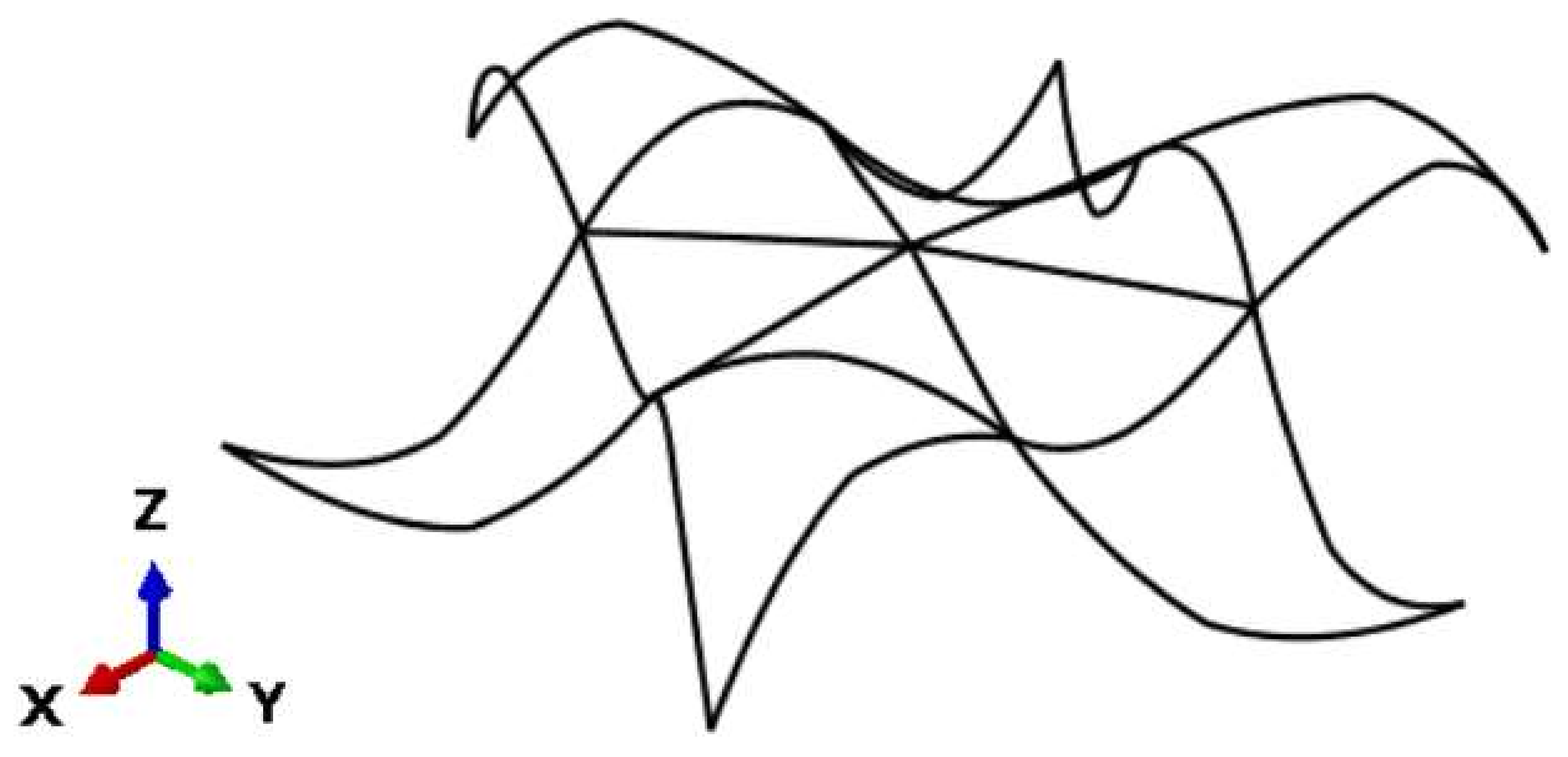
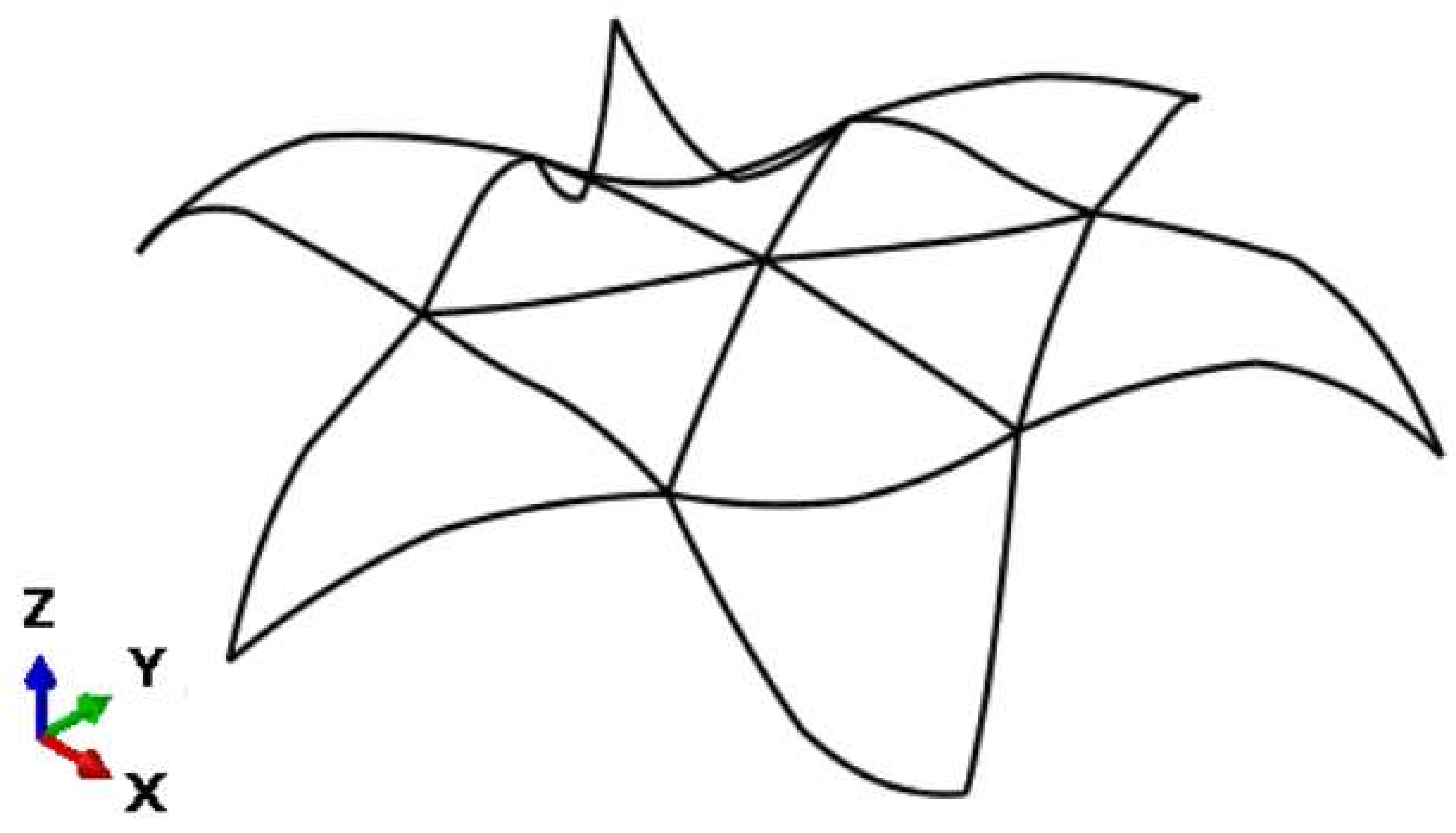
In the dynamic analysis of each structure, the knowledge of its dynamic characteristics is of primary interest. The natural frequencies and modes of vibration, which are usually needed, are obtained after solving the appropriate linear eigenvalue problem [2]. This is a standard procedure. In the context of the dynamics of reticulated domes (treated as undamped systems), some information about the frequencies and modes of vibration can be found in [10,12,29,37], usually as a description of the dynamic characteristics of the considered domes. Only paper [37] is related to the determination of some specific modes of vibration. Papers related to the determination of the dynamic characteristics of damped reticulated domes are very rare. In paper [16], the damping ratios and modes of vibration of small domes are analyzed numerically and compared with experimental results. The complex model and the Rayleigh model were used to theoretically describe the damping effects. The damping ratios and natural frequencies are also determined experimentally in [35] for a small dome supported on the isolation devices. Typical experimental values of damping ratios are of the order 0.002–0.003, according to the paper [16], and damping ratios of the order 0.01–0.02 are reported in [35]. Moreover, in the paper [17], the effects of the nonlinear material loss factor on the damping properties of latticed domes are investigated.

If the passive control system consisting, for example, of VE dampers is installed on the structure, design engineers are also interested in the determination of the modal, non-dimensional damping ratio or the modal loss factors and the frequency response functions (in short, FRFs). The non-dimensional damping ratios (or the modal loss factors) are a measure of the possibility of energy dissipation when the structure vibrates in a particular mode of vibration. The nonlinear eigenvalue problem (NEP), such as the one presented in [2,4], must be solved when the above-mentioned damping ratios (loss factors), natural frequencies and modes of vibration are of interest. In this context, Horr et al. [38,39] and Lewandowski et al. [40] proposed a spectral finite element analysis method for structures made of homogeneous (not composite) VE rods.

However, to the best of our knowledge, the dynamic characteristics of reticulated domes with VE elements (VE dampers and/or VE layers on the dome’s rod) are not analyzed at all. The above brief review of the literature clearly shows a lack of a systematic analysis of the dynamic characteristics of reticulated domes. The main aim of this paper is to fill this gap, at least partially. For this reason, and in order to fill this gap, the principal aim of this paper is to propose a new formulation for domes made of rods which are built of two parts, i.e., the first part is made of an elastic material and the second part is made of a VE material. Moreover, the above-mentioned NEP from which the dynamic characteristics can be determined is derived. The continuation method is used for the sole NEP.

The paper is organized as follows. After a short review of the existing open literature in Section 1, the dynamic analysis of a rod with VE layers is presented in Section 2. An analysis of the free vibration of the whole dome and a description of the continuation method used to solve NEP are presented in Section 3. Section 4 contains an analysis of the steady-state vibration of the dome as well as information on the determination of the FRFs. The results of a representative calculation are presented and briefly discussed in Section 5. Concluding remarks are found in Section 6. The paper also contains a few appendices where some detailed derivations are presented.

2. Dynamic Analysis of Viscoelastic (VE) Rods

The considered rod is a composite one. It is built of two parts, one of which is elastic and one is VE. In the context of reticulated domes, typical examples of elastic materials are steel and/or aluminum. The examples of VE materials that can be used to dissipate vibration energy and for which the presented theory is valid are different types of polymers and elastomers. The purely elastic Part #1 has the elastic modulus $E_s$ and density ${\rho }_s$. Part #2 is VE with density ${\rho }_v$, has a much higher loss factor than Part #1 and is modeled with the help of the fractional Zener model. The model consists of four parameters, i.e., the relaxed elastic modulus $E_0$ and $G_0$, the non-relaxed elastic modulus $E_{\infty }$ and $G_{\infty }$, the relaxation time $\tau$ and the order of the fractional derivative $\alpha$ ($0<\alpha \le 1$). Moreover, it is assumed that the Poisson ratio $\nu$ is constant, i.e., it is independent of the frequency of excitation, the temperature and the amplitude of vibration. Additionally, it is assumed that the relationships between the moduli are

$$G_0=\frac{1}{2}{E}_0/(1+\nu ), G_{\infty }=\frac{1}{2}{E}_{\infty }/(1+\nu ).$$

Of course, real “elastic” materials also have loss factors, but, for example, metals have low loss factors (in the order of ${10}^{-3}$), which will be neglected here in comparison with the loss factors of the VE part of the rod.

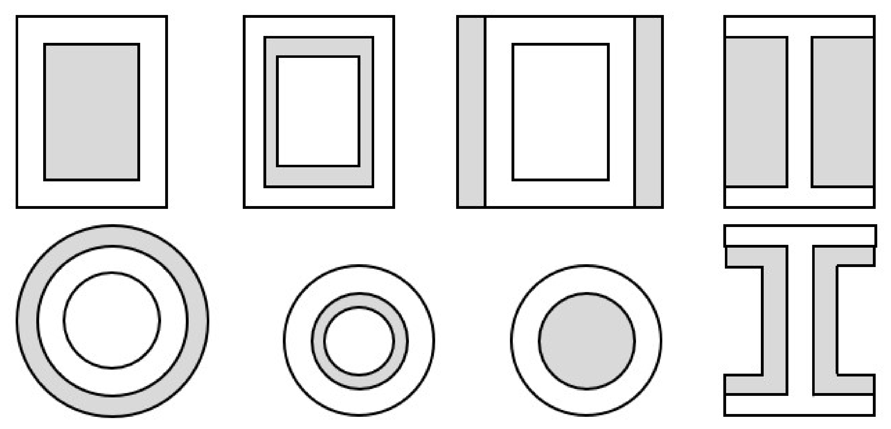
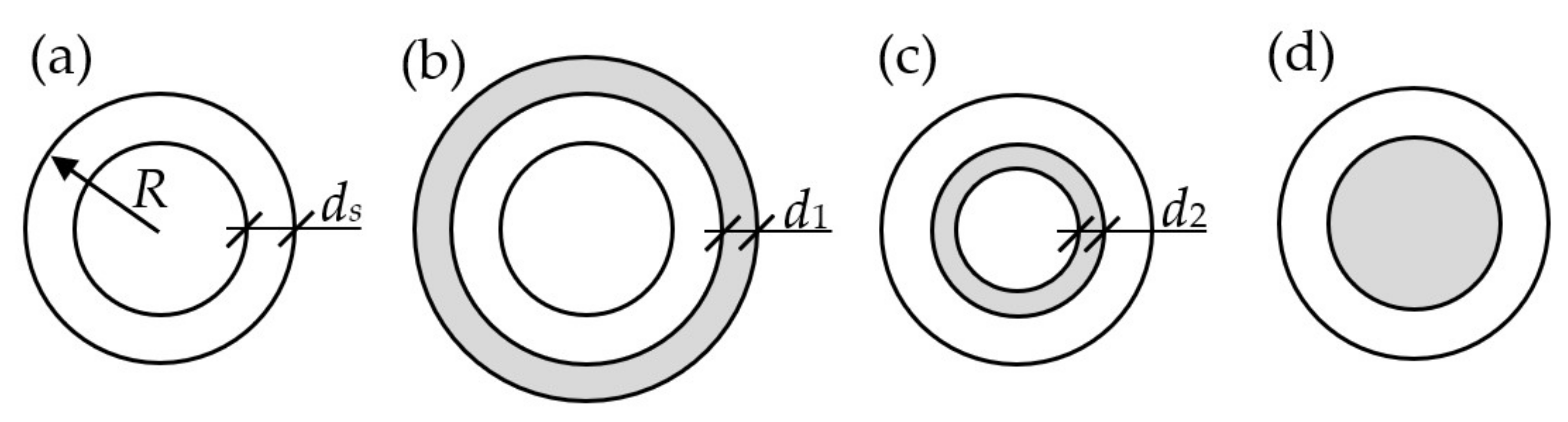
The rod in a three-dimensional space is considered, which could be stretched/pressed, sheared, bended and twisted. For these reasons, the Timoshenko theory is used as the model of the rod. The cross-section of the rod has two axes of symmetry and contains the elastic and the VE parts. It is assumed that the structure built of the elastic part of a rod only is geometrically stable. The interface of the elastic and the VE parts is no-slip. Both parts have the center of gravity in the same point in space. The plane cross-section in each part remains as a plane after deformation. This assumption agrees with the one used in the well-known Ross, Kerwin and Ungar theory (briefly, the RKU theory) [41,42]. Moreover, the VE material is rheologically simple, which means that the correspondence principle could be used. All rods in a dome are built of an identical VE material. Examples of the possible cross-section of the VE rods are shown in Figure 1, where the VE part of the cross-section is shown as the grey area.

The considered rod in a three-dimensional space is shown in Figure 2, where the positive end displacements of the rod are also visible. The theory presented in [43] is adopted to describe the dynamic behavior of the rod. This finite element with six degrees of freedom has three displacements and three rotations (see Figure 2) at one node. It is assumed that the displacements and the rotations are small. Therefore, the displacements $u(x,y,z,t)$, $v(x,y,z,t)$ and $w(x,y,z,t)$ of a freely chosen point of the rod can be expressed as [43]:

$$u(x,y,z,t)=u_c(x,t)-{\varphi }_z(x,t)y+{\varphi }_y(x,t) z,$$

(1)

$$v(x,y,z,t)=v_c(x,t)-{\varphi }_x(x,t) z,$$

(2)

$$w(x,y,z,t)=w_c(x,t)+{\varphi }_x(x,t) y,$$

(3)

where $u_c(x,t)$, $v_c(x,t)$ and $w_c(x,t)$ are the displacements of the rod axis, and ${\varphi }_x(x,t)$, ${\varphi }_y(x,t)$ and ${\varphi }_z(x,t)$ are rotations (see Figure 2 for details).

The nonzero strains for the considered rod are the following functions of displacements and rotations (see [43]):

$${\epsilon }_{xx}(x,y,z,t)=u_{c,x}(x,t)-y{\varphi }_{z,x}(x,t)+z{\varphi }_{y,x}(x,t),$$

(4)

$${\epsilon }_{xy}(x,y,z,t)=v_{c,x}(x,t)-z{\varphi }_{x,x}(x,t)-{\varphi }_z(x,t),$$

(5)

$${\epsilon }_{xz}(x,y,z,t)=w_{c,x}(x,t)+y{\varphi }_{x,x}(x,t)+{\varphi }_y(x,t),$$

(6)

where $t$ is the time, ${(•)}_{,x}=d(•)/dx$ and $u_c(x,t)$, $v_c(x,t)$ and $w_c(x,t)$ are the displacement of a freely chosen point at the rod axis. Later in this paper, the subscript $c$ is dropped, and $u(x,t)$, $v(x,t)$ and $w(x,t)$ will be used to denote displacements at the rod axis.

Moreover, the following generalized strains are introduced: the axial strain $\epsilon (x,t)$, the curvature in the x0y plane ${\kappa }_y(x,t)$, the curvature in the x0z plane ${\kappa }_z(x,t)$, the shear strains ${\gamma }_y(x,t)$ and ${\gamma }_z(x,t)$ and the torsional rate ${\kappa }_x(x,t)$. These quantities are defined as follows:

$$\epsilon (x,t)=u_{,x}(x,t),$$

(7)

$${\kappa }_y(x,t)=-{\varphi }_{z,x}(x,t), {\kappa }_z(x,t)={\varphi }_{y,x}(x,t),$$

(8)

$${\gamma }_y(x,t)=v_{,x}(x,t)-{\varphi }_z(x,t), {\gamma }_z(x,t)=w_{,x}(x,t)+{\varphi }_z(x,t),$$

(9)

$${\kappa }_x(x,t)={\varphi }_{x,x}(x,t).$$

(10)

Based on the quantities introduced above, the vector of displacements

$$w_e(x,t)={[u(x,t),v(x,t),w(x,t),{\varphi }_x(x,t),{\varphi }_y(x,t),{\varphi }_z(x,t)]}^T$$

and the vector of generalized strains

$$e_e(x,t)={[\epsilon (x,t),{\kappa }_y(x,t),{\kappa }_z(x,t),{\gamma }_y(x,t),{\gamma }_z(x,t),{\kappa }_x(x,t)]}^T$$

are defined. Moreover, the vector of internal forces is introduced:

$$s_e(x,t)={[N(x,t),M_z(x,t),M_y(x,t),T_y(x,t),T_z(x,t),M_x(x,t)]}^T$$

The symbols in the definition above denote the axial force, the bending moments, the shear forces and the torsional moment, respectively. Definitions of internal forces are given in Appendix A. It should be noted that the internal forces are a sum of forces in both parts of the rod.

The virtual work equation for the considered finite element is

$$\delta q_e^T(t)R_e(t)+{\displaystyle \underset{0}{\overset{l_e}{\int }}\delta w_e^T(x,t)b_e(x,t)dx}+{\displaystyle \underset{0}{\overset{l_e}{\int }}\delta w_e^T(x,t)p_e(x,t)dx}={\displaystyle \underset{0}{\overset{l_e}{\int }}\delta e_e^T(x,t)s_e(x,t)dx}$$

(11)

where the symbol $\delta (•)$ means that the following quantity $(•)$ is the virtual one, and $l_e$ is the length of the element. The vector of inertial forces $b_e(x,t)$ per unit length of the element and the vector of excitation forces $p_e(x,t)$ are detailed in Appendix A. Moreover, the vector of nodal forces is denoted by $R_e(t)$, and $q_e(t)$ is the vector of nodal parameters.

Proceeding in a conventional way, the virtual work of inertial forces could be written in the following form

$$L_b=-{\displaystyle \underset{0}{\overset{l_e}{\int }}\delta w_e^T(x,t)m_e{\ddot{w}}_e(x,t)dx},$$

(12)

where the matrix $m_e$ is given by (B6). Details of derivation are presented in Appendix B.

The analysis of the virtual work of internal forces is more complex because the constitutive equation for the VE material is a fractional differential equation. Details are presented in Appendix C. Therefore, the virtual work of internal forces can be temporarily written in the following form:

$$L_i={\displaystyle \underset{0}{\overset{l_e}{\int }}\delta {\epsilon }_e^T(x,t)E_s{e}_e(x,t)dx}+{\displaystyle \underset{0}{\overset{l_e}{\int }}\delta {\epsilon }_e^T(x,t)s_{ev}(x,t)dx},$$

(13)

where $s_{ev}(x,t)$ is the resultant inertial forces obtained from the VE part of the rod and quantities $E_s$ are the constitutive matrix connected with the elastic part of the rod.

Two types of dynamic problems of the dome are considered in particular, i.e., the free vibration problem and the steady-state vibration of the dome, excited by harmonically varying forces.

In the case of free vibration $p_e(x,t)=0$ and the Laplace transform (with zero initial conditions) applied to the virtual work, Equation (11) gives the relationship:

$$\delta {\tilde{q}}_e^T{\tilde{R}}_e-s^2{\displaystyle \underset{0}{\overset{l_e}{\int }}\delta {\tilde{w}}_e^T(x)m_e{\tilde{w}}_e(x)dx}={\displaystyle \underset{0}{\overset{l_e}{\int }}\delta {\tilde{e}}_e^T(x)[E_s+E_0+\theta (s)\Delta E] {\tilde{e}}_e(x)dx},$$

(14)

where the wave over the quantities means that it is their Laplace transform, and relationships (12) and (C7) are also taken into account.

The finite element method is adopted to discretize displacements, and according to this method:

$${\tilde{w}}_e(x)=N(x){\tilde{q}}_e,$$

(15)

where ${\tilde{q}}_e$ is the vector of the Laplace transform of nodal parameters and $N(x)$ is the matrix of shape functions. Moreover, it is well known that

$${\tilde{e}}_e(x)=B(x){\tilde{q}}_e.$$

(16)

By introducing (15) and (16) in (14) and remembering that the virtual state can be freely chosen, the following equation is obtained:

$${\tilde{R}}_e=[s^2{M}_e+K_{es}+\theta (s)K_{ev}]{\tilde{q}}_e,$$

(17)

where $M_e$, $K_{es}$ and $K_{ev}$ are the mass matrix, the elastic stiffness matrix and the VE stiffness matrix, defined as:

$$M_e={\displaystyle \underset{0}{\overset{l_e}{\int }}{N}_e^T(x)m_e{N}_e(x)dx}, K_{es}={\displaystyle \underset{0}{\overset{l_e}{\int }}{B}_e^T(x)[E_s+E_0]B_e^T(x)dx},$$

(18)

$$K_{ev}={\displaystyle \underset{0}{\overset{l_e}{\int }}{B}_e^T(x)\Delta EB(x)dx}.$$

(19)

It should be noted that the elastic stiffness matrix comprises the influence of both the elastic part of the rod (through matrix $E_s$) and the elastic properties of the VE part of the rod (through matrix $E_0$).

The commercial program Abaqus, along with the beam finite element B32, is used to calculate the elemental matrices $M_e$, $K_{es}$, $K_{ev}$ and the corresponding global ones.

The steady-state harmonically varied vibration is analyzed because the FRF, which is one of the dynamic characteristics of structures, could easily be obtained. Now, the considered finite element is excited by the harmonically varying forces described as

$$p_e(x,t)=p_{ec}(x)\cos \lambda t+p_{es}(x)\sin \lambda t={\overline{p}}_{e1}(x)e^{\mathrm{i}\lambda t}+p_{e1}(x)e^{-\mathrm{i}\lambda t}$$

(20)

where $\lambda$ is the angular excitation frequency, and $p_{ec}(x)$ and $p_{es}(x)$ are vectors of the real “amplitudes” of excitation forces. Moreover, ${\overline{p}}_{e1}(x)=\frac{1}{2}(p_{ec}(x)-\mathrm{i}{p}_{es}(x))$, and $p_{e1}(x)=\frac{1}{2}(p_{ec}(x)+\mathrm{i}{p}_{es}(x))$.

Vibrations of the rod in the steady state can be described as follows:

$$w_e(x,t)=N(x)q_e(t),$$

(21)

$$q_e(t)={\overline{q}}_{e1}T(\lambda )+q_{e1}\overline{T}(\lambda ),$$

(22)

where $T_1(\lambda )=e^{\mathrm{i}\lambda t}$ and ${\overline{T}}_1(\lambda )=e^{-\mathrm{i}\lambda t}$. In this part of the paper, the bar over the quantity means that it is a complex conjugate one in comparison with the same quantity without a bar.

The time average virtual work equation (instead of (11)) is used in the steady-state analysis. The above-mentioned equation has the following form:

$$\begin{array}{l}\frac{1}{T}{\displaystyle \underset{0}{\overset{T}{\int }}\delta q_e^T(t)R_e(t)dt}+\frac{1}{T}{\displaystyle \underset{0}{\overset{T}{\int }}{\displaystyle \underset{0}{\overset{l_e}{\int }}\delta w_e^T(x,t)b_e(x,t)dx}dt}+\\ \hspace{1em}\hspace{1em}\hspace{1em}\frac{1}{T}{\displaystyle \underset{0}{\overset{T}{\int }}{\displaystyle \underset{0}{\overset{l_e}{\int }}\delta w_e^T(x,t)p_e(x,t)dx}dt}=\frac{1}{T}{\displaystyle \underset{0}{\overset{T}{\int }}{\displaystyle \underset{0}{\overset{l_e}{\int }}\delta e_e^T(x,t)s_e(x,t)dx}dt}\end{array}$$

(23)

where $T=2\pi /\lambda$ is the period of excitation forces.

The time changes of virtual displacements are assumed to be in the form:

$$\delta w_e(x,t)=N(x)\delta q_e(t),$$

(24)

$$\delta q_e(t)=\delta {\overline{q}}_{e1}T(\lambda )+\delta q_{e1}\overline{T}(\lambda ).$$

(25)

The real and virtual generalized strains are discretized as follows:

$$e_e(x,t)=B_e(x)q_e(t),$$

(26)

$$\delta e_e(x,t)=B_e(x)\delta q_e(t).$$

(27)

A detailed analysis of the averaged virtual work equation is presented in Appendix D. Finally, this equation can be rewritten in the following form:

$$\begin{array}{ll}\hfill \delta {\overline{q}}_{e1}^T{R}_{e1}+& \delta q_{e1}^T{\overline{R}}_{e1}=\hfill \\ & \delta {\overline{q}}_{e1}^T[K_{es}+{\overline{\theta }}_1(\tau \lambda )K_{ev}-{\lambda }^2{M}_e]q_{e1}+\delta {\overline{q}}_{e1}^T{P}_{e1}+\hfill \\ & \delta q_{e1}^T[K_{es}+{\theta }_1(\tau \lambda )K_{ev}-{\lambda }^2{M}_e]{\overline{q}}_{e1}+\delta q_{e1}^T{\overline{P}}_{e1}\hfill \end{array}$$

(28)

The virtual displacements could be freely chosen, and, for this reason, Equation (28) is fulfilled when the following two equalities hold:

$$R_{e1}=[K_{es}+{\overline{\theta }}_1(\tau \lambda )K_{ev}-{\lambda }^2{M}_e]q_{e1}-P_{e1},$$

(29)

$${\overline{R}}_{e1}=[K_{es}+{\theta }_1(\tau \lambda )K_{ev}-{\lambda }^2{M}_e]{\overline{q}}_{e1}-{\overline{P}}_{e1}.$$

(30)

3. Analysis of the Free Vibration of the Dome

3.1. General Information Concerning NEP

With the elemental Equation (17), and using the well-known finite element procedure, it is possible to obtain the following equation:

$$D(s)\tilde{q}\equiv ⎣K_s+\theta (s)K_v+s^{2}M⎦ \tilde{q}=0,$$

(31)

for the whole dome, where $\tilde{q}$ is the Laplace transform of the global vector of nodal parameters, and the global mass and stiffness matrices $M$, $K_s$, $K_v$ are built in the usual way using the elemental matrices $M_e$, $K_{es}$, $K_{ev}$, defined by (18), (19) and the transformation matrix $T_e$ from local to global coordinate systems. Moreover, $D(s)=K_s+\theta (s)K_v+s^{2}M$.

From the mathematical point of view, Equation (31) is the NEP with $s$ as the eigenvalue, and the vector $\tilde{q}$, previously described as the Laplace transform of $q$, is now treated as the eigenvector.

In general, eigenvalues can be complex numbers or real numbers. Similarly, eigenvectors can also be complex or real vectors. When the VE properties of a material are described with the help of the fractional Zener model, it can be proved that eigenvalues and eigenvectors that are the solution to (31) are only the complex eigenvalues and eigenvectors [4,44]. The NEP (31) has $2n$ solutions, where $n$ is the number of the degree of freedom of the dome. Only a few initial solutions are interesting from the practical point of view.

If there is a complex solution, then there is also a complex, conjugate solution coupled with it, i.e., if the solution is $s=\mu +\mathrm{i}\eta$ and $\tilde{q}(s)=a+ib$, where $a$ and $b$ are real vectors, then the solution is also $s=\mu -i\eta$ and $\tilde{q}(s)=a-ib$. Moreover, in all cases, $\mu <0$.

The solution to NEP is not an easy task. However, there are a number of methods to solve the problem. An interesting survey of NEP associated with matrix-valued functions which depend nonlinearly on a parameter is presented in [44,45,46]. A few methods based on successive linearization were proposed by Ruhe in [47] in order to solve the NEP problem. In [48], Singh proposed a method to solve NEP based on Newton’s eigenvalue iteration. An asymptotic method to solve NEP and calculate the dynamic characteristics of a VE system is proposed in [49]. Moreover, the continuation method, also known as the homotopy method, is used in [4,50,51,52,53] to solve NEP arising in the dynamics of VE systems. An iterative algorithm, a first-order perturbation method and a reduced basis technique are used by Chen et al. [54] to solve the NEP. In [55], two iterative algorithms to solve NEP were developed. These methods combine homotopy, the asymptotic numerical technique and Padé approximants. Recently, a new iterative method which used first-order perturbation was proposed in [56] for the determination of the eigenvalues and eigenvectors of nonviscously damped vibration systems. However, for large NEP, the direct use of the continuation method for a set of eigenvalues and eigenvectors is time-consuming. One possible way to reduce the total computation time is to reduce the NEP order before proceeding to its solution. For this reason, an application of the subspace iteration method to solve NEP is proposed, as described in [57,58].

Two versions of the continuation method, described below, were adopted to solve the considered NEP.

3.2. The Classical Continuation Method for NEP

The classical continuation method adopted to solve NEP (31) was previously successfully used in [4,40,50,52] and will be briefly repeated here for the reader’s convenience and for the completeness of the description of the numerical procedure.

In (31), there are n equations with n + 1 unknowns, and, for this reason, an additional equation called the constraint equation, assumed here in the form

$$\frac{1}{2} {\tilde{q}}^T{D}_{,s}(s)\tilde{q}-a=0,$$

(32)

must be added, where

$$D_{,s}(s)=\frac{\partial D}{\partial s}=2sM+\frac{\mathrm{d}\theta }{\mathrm{d}s}{K}_v,$$

(33)

$$\frac{\mathrm{d}\theta }{\mathrm{d}s}=\frac{\alpha {\tau }^{\alpha }{(s\tau )}^{\alpha -1}}{{[1+{(s\tau )}^{\alpha }]}^2},$$

(34)

The constraint equation can also be understood as a way of normalizing the vector $\tilde{q}$.

The artificial continuation parameter $0\le \kappa \le 1$ is now introduced, and Equations (31) and (32) are rewritten in the form of

$$h_1(s,\tilde{q})\equiv D(s,\kappa )\tilde{q}\equiv ⎣K_s+\kappa \theta (s)K_v+s^{2}M⎦ \tilde{q}=0,$$

(35)

$$h_2(s,\tilde{q})\equiv \frac{1}{2} {\tilde{q}}^T{D}_{,s}(s,\kappa )\tilde{q}-a=0.$$

(36)

It should be noted that, for $\kappa =0$, (35) reduced to the following linear eigenvalue problem:

$$(K_s+s^{2}M) \tilde{q}=0,$$

(37)

while, for $\kappa =1$, (35) is identical with (31). The idea of the continuation method is to create a series of solutions of (35) for different values of $\kappa$, starting from $\kappa =0$ and ending the continuation process at $\kappa =1$.

There are many efficient numerical procedures and commercial programs which can be used to efficiently solve the linear eigenvalue problem (37). From the practical point of view, only the first few eigenvalues and eigenvectors of (37) are of interest. One is for the chosen eigenvalues $s=\mathrm{i}{\omega }^2$ and the corresponding eigenvector $\tilde{q}=a$, where $\omega$ and $a$ are the natural frequency and the mode of vibration of the dome for which elastic properties are taken into account. These quantities are the starting approximation of NEP (31) for $\kappa =0$, which is denoted by

$$s_0=0+\mathrm{i}\omega , {\tilde{q}}_0=a+\mathrm{i}0,$$

(38)

where the lower index in (38) indicates that it is the solution to (35) for ${\kappa }_0=0$.

Let us assume that the solution to (35), denoted as $s_{k-1}$ and ${\tilde{q}}_{k-1}$, is known for some specific value of the continuation parameter denoted as ${\kappa }_{k-1}$. Our aim is to obtain the solution to NEP (35) for the next values of the continuation parameter, i.e., for ${\kappa }_k={\kappa }_{k-1}+\Delta \kappa$, where $\Delta \kappa$ is the assumed increment of the continuation parameter.

In the considered incremental step, a set of nonlinear equations, (35) and (36), must be solved. This is usually solved with the help of the Newton method. The Newton method is an iterative one which requires the updating of the tangent matrix in each iteration. During the iteration process, it is assumed that, at the beginning of iteration number $i$, we know some approximation of the searched solution denoted here by $s_k^{(i)}$, ${\tilde{q}}_k^{(i)}$, and our aim is to determine a better approximation of the solution. According to the Newton method, the following set of linearized equations must be solved with respect to $\Delta s$ and $\Delta \tilde{q}$:

$$\left[\begin{array}{cc}\mathbf{D}\left(s_k^{\left(i\right)},{\kappa }_k\right)\hfill & {\mathbf{D}}_{,s}\left(s_k^{\left(i\right)},{\kappa }_k\right){\tilde{\mathbf{q}}}_k^{\left(i\right)}\hfill \\ {\tilde{\mathbf{q}}}_k^{{\left(i\right)}^T}{\mathbf{D}}_{,s}\left(s_k^{\left(i\right)},{\kappa }_k\right)\hfill & \frac{1}{2}{\tilde{\mathbf{q}}}_k^{\left(i\right)}{\mathbf{D}}_{,ss}\left(s_k^{\left(i\right)},{\kappa }_k\right){\tilde{\mathbf{q}}}_k^{\left(i\right)}\hfill \end{array}\right]\left\{\begin{array}{c}\Delta \tilde{\mathbf{q}}\hfill \\ \Delta s\hfill \end{array}\right\}=-\left\{\begin{array}{c}{\mathbf{h}}_1\left(s_k^{\left(i\right)},{\tilde{\mathbf{q}}}_k^{\left(i\right)},{\kappa }_k\right)\hfill \\ h_2\left(s_k^{\left(i\right)},{\tilde{\mathbf{q}}}_k^{\left(i\right)}\right)\hfill \end{array}\right\},$$

(39)

where

$$D_{,ss}(s,\kappa )=2M+\frac{{\mathrm{d}}^2\theta (s)}{\mathrm{d}{s}^2}{K}_v,$$

(40)

$$\frac{{\mathrm{d}}^2\theta (s)}{\mathrm{d}{s}^2}=\frac{\alpha (\alpha -1)s^{\alpha -2}{\tau }^{\alpha }-2{\alpha }^2{s}^{2(\alpha -1)}[1+{(s\tau )}^{\alpha }]}{{[1+{(s\tau )}^{\alpha }]}^4}.$$

(41)

A next approximation of the searched solution is given by:

$$s_k^{(i+1)}=s_k^{(i)}+\Delta s, {\tilde{q}}_k^{(i+1)}={\tilde{q}}_k^{(i)}+\Delta \tilde{q}.$$

(42)

The iteration is repeated until the following inequalities are fulfilled:

$$\left|\Delta s\right|\le {\epsilon }_1\left|s_k^{(i+1)}\right|, ‖\Delta \tilde{q}‖\le {\epsilon }_2‖{\tilde{q}}_k^{(i+1)}‖, ‖D(s)\tilde{q}‖\le {\epsilon }_3‖K_s\tilde{q}‖,$$

(43)

where ${\epsilon }_1={\epsilon }_2=0.0001$ and ${\epsilon }_3=0.001$ are the assumed accuracies of calculations. The last obtained approximation of the NEP solution is the searched solution for ${\kappa }_k$, i.e., $s_k=s_k^{(i+1)}$, ${\tilde{q}}_k={\tilde{q}}_k^{(i+1)}$.

The incremental process is repeated until the solution to (35) for $\kappa =1$ is obtained, which is also the solution to NEP (31).

With the eigenvalue $s=\mu +\mathrm{i}\eta$, the corresponding natural frequency $\omega$ and damping ratio $\gamma$ could be calculated from

$${\omega }^2={\mu }^2+{\eta }^2, \gamma =-\mu /\omega .$$

(44)

In this way, one solution to NEP (31) is found, and the natural frequency and damping ratio can be calculated.

The incremental–iterative process described above must be repeated if more solutions are required.

3.3. The Continuation Method Proposed by Jarlebring et al. [59]

Some improvements in the Newton iterative procedure used to solve NEP were proposed by Jarlebring et al. in [59], where a quasi-Newton procedure is used instead of the full Newton approach.

The above-mentioned procedure was successfully applied in [60] and will be adopted here as one element of the continuation method used to solve NEP (31). First of all, the so-called continuation parameter, $\kappa$ ($0\le \kappa \le 1$), is introduced, and NEP (31) is rewritten in the form of Equation (35).

In the method described here, the constraint equation is chosen in the following form:

$$h_2(s,\tilde{q})=c^T\tilde{q}-a=0,$$

(45)

where $c$ is the assumed vector and $a$ is the known constant whose value will be specified later. Very often, $c$ is a unit vector or $c={[0, 0, 0, 0, 0, 1, 0, 0, 0, 0]}^T$, where 1 is in a freely chosen position in $c$.

Let us assume that the solution to (35), denoted as $s_{k-1}$ and ${\tilde{q}}_{k-1}$, is known for some specific value of the continuation parameter denoted as ${\kappa }_{k-1}$. As in the previously presented method, our aim is to obtain the solution to NEP (35) for the next values of the continuation parameter, i.e., for ${\kappa }_k={\kappa }_{k-1}+\Delta \kappa$, where $\Delta \kappa$ is the assumed increment of the continuation parameter.

In the considered incremental step, a set of nonlinear equations, (35) and (45), must be solved now. It is usually solved with the help of the “full” Newton method. The “full” Newton method is an iterative one which requires the updating of the tangent matrix in each iteration. During the iteration process, it is assumed that, at the beginning of iteration number $i$, we know some approximation of the solution sought, which is denoted here by $s_k^{(i)}$, ${\tilde{q}}_k^{(i)}$, and our aim is to determine a better approximation of the solution. According to the “full” Newton method, the following set of linearized equations must be solved with respect to $\Delta s$ and $\Delta \tilde{q}$:

$$\left[\begin{array}{cc}\mathbf{D}\left(s_k^{\left(i\right)},{\kappa }_k\right)& {\mathbf{D}}_{,s}\left(s_k^{\left(i\right)},{\kappa }_k\right){\tilde{\mathbf{q}}}_k^{\left(i\right)}\\ {\mathbf{c}}^T& 0\end{array}\right]\left\{\begin{array}{c}\Delta \tilde{\mathbf{q}}\hfill \\ \Delta s\hfill \end{array}\right\}=-\left\{\begin{array}{c}{\mathbf{h}}_1\left(s_k^{\left(i\right)},{\tilde{\mathbf{q}}}_k^{\left(i\right)},{\kappa }_k\right)\hfill \\ h_2\left(s_k^{\left(i\right)},{\tilde{\mathbf{q}}}_k^{\left(i\right)}\right)\hfill \end{array}\right\}.$$

(46)

In [59], Jarlebiring et al. proposed some improvements of the “full” Newton method which save a considerable amount of computational time. The main idea is to calculate the matrix $D(s_k^{(i)},{\kappa }_k)$ only once at the beginning of the iterative process and keep this matrix unchanged during the iteration process. This means that we have the matrix $D(s_k^{(0)}=s_{k-1},{\kappa }_k)$ in the place of $D(s_k^{(i)},{\kappa }_k)$ for all iterations. Moreover, the set of Equations (46) is solved in the specific way described below.

After the above-mentioned change in Equation (46)(1) and the multiplication of (46)(1) by $c^T{D}^{-1}(s_{k-1},{\kappa }_k)$, we obtain

$$\begin{array}{l}{c}^T{D}^{-1}(s_{k-1},{\kappa }_k)D(s_{k-1},{\kappa }_k)\Delta \tilde{q}+c^T{D}^{-1}(s_{k-1},\kappa {\kappa }_k)D_{,s}(s_k^{(i)},{\kappa }_k){\tilde{q}}_k^{(i)}\Delta s=\\ -c^T{D}^{-1}(s_{k-1},\kappa {\kappa }_k)h_1(s_k^{(i)},{\tilde{q}}_k^{(i)},{\kappa }_k).\end{array}$$

(47)

The first term of (47) could be rewritten as $c^T\Delta \tilde{q}$ and is equal to zero because of the way of normalizing the eigenvector $\tilde{q}$. This also means that, from (47), we obtain

$$\Delta s=-\frac{c^T{D}^{-1}(s_{k-1},{\kappa }_k)h_1(s_k^{(i)},{\tilde{q}}_k^{(i)},{\kappa }_k)}{c^T{D}^{-1}(s_{k-1},\kappa {\kappa }_k)D_{,s}(s_k^{(i)},{\kappa }_k){\tilde{q}}_k^{(i)}}.$$

(48)

With $\Delta s$, it is possible to calculate a new approximation of the eigenvalue, i.e., $s_k^{(i+1)}=s_k^{(i)}+\Delta s$.

Formula (48) is numerically performed in such a way that, first of all, the additional vector $u(s_{k-1})$ is determined as a solution to the following equation:

$$D(s_{k-1},{\kappa }_k)u(s_{k-1})=c,$$

(49)

and after that, (48) can be rewritten in the following form:

$$\Delta s=-\frac{u^T(s_{k-1})h_1(s_k^{(i)},{\tilde{q}}_k^{(i)},{\kappa }_k)}{u^T(s_{k-1})D_{,s}(s_k^{(i)},{\kappa }_k){\tilde{q}}_k^{(i)}}.$$

(50)

Now, after the multiplication of (46.1) by $D^{-1}(s_{k-1},{\kappa }_k)$, and taking into account that $D^{-1}(s_{k-1},{\kappa }_k)D(s_{k-1},{\kappa }_k)=I$, a new approximation of the eigenvector ${\tilde{q}}_k$ is obtained from the following formula:

$$\Delta \tilde{q}=-D^{-1}(s_{k-1},{\kappa }_k) z^{(i)},$$

(51)

$${\tilde{q}}_k^{(i+1)}={\tilde{q}}_k^{(i)}+\Delta \tilde{q},$$

(52)

where

$$z^{(i)}=[D_{,s}(s_k^{(i)},{\kappa }_k){\tilde{q}}_k^{(i)}\Delta s+h_1(s_k^{(i)},{\tilde{q}}_k^{(i)},{\kappa }_k)].$$

(53)

It should be noted that, in (53), there appears the actual iterative change of the eigenvalue $\Delta s$, which is determined from (48) or (50).

In order to avoid the inversion of the matrix $D(s_{k-1},{\kappa }_k)$, relationship (51) could be written in the following form:

$$D(s_{k-1},{\kappa }_k)\Delta \tilde{q}=-z^{(i)}.$$

(54)

After each iteration, the actual approximation of the eigenvector (i.e., vector ${\tilde{q}}_k^{(i+1)}$) obtained from (52) must be normalized in order to fulfill the normalization criterion (45).

The iteration is repeated until the inequalities (43) are fulfilled. The last-obtained approximation of the NEP solution is the solution sought for ${\kappa }_k$, i.e., $s_k=s_k^{(i+1)}$${\tilde{q}}_k={\tilde{q}}_k^{(i+1)}$.

The incremental process is repeated until the solution to (46.1) for $\kappa =1$ is obtained, and it is also the solution to NEP (31). The corresponding natural frequency $\omega$ and damping ratio $\gamma$ could be calculated from (44). As in the previous method, the incremental–iterative process described above must be repeated if more solutions are needed.

4. Analysis of the Steady-State Vibration of the Dome and the Determination of Frequency Response Functions (FRF)

In the analysis of steady-state vibration, the global amplitude equations are obtained using the well-known finite element procedure and using the elemental Equations (29) and (30). The final results are

$$[K_s+{\overline{\theta }}_1(\tau \lambda )K_v-{\lambda }^{2}M]q_1=P_1,$$

(55)

$$[K_s+{\theta }_1(\tau \lambda )K_v-{\lambda }^{2}M]{\overline{q}}_1={\overline{P}}_1,$$

(56)

where the global matrices $M$, $K_s$ and $K_v$ are generated in the usual way using the elemental matrices $M_e$, $K_{es}$ and $K_{ev}$, respectively, and the transformation matrix $T_e$ from the local coordinate systems to the global one. The global vectors of the “amplitudes” of the excitation forces $P_1$ and ${\overline{P}}_1$ are generated using the elemental vectors of the “amplitudes” of the excitation forces $P_{e1}$ and ${\overline{P}}_{e1}$. Moreover, $q_1$ and ${\overline{q}}_1$ are the global vectors of complex, conjugate vectors of the “amplitudes” of nodal parameters, whereas the quantities ${\overline{\theta }}_1(\tau \lambda )$ and ${\theta }_1(\tau \lambda )$ are defined in Appendix D.

It should be noted that only one of Equation (55) or (56) must be solved, because the above-mentioned vectors $q_1$ and ${\overline{q}}_1$ are complex and conjugate. For the given excitation forces, the response curves are obtained by solving the amplitude equation for a set of excitation frequencies taken from the assumed range of ${\lambda }_{\min }\ge \lambda \ge {\lambda }_{\max }$.

If, for a specific value of excitation frequency, vectors $q_1=q_r+\mathrm{i}{q}_i$ and ${\overline{q}}_1=q_r-\mathrm{i}{q}_i$ are known, then the steady-state solution can also be written in terms of trigonometric functions, i.e.,

$$q(t)=q_c\cos \lambda t+q_s\sin \lambda t,$$

(57)

where $q_c=q_1+{\overline{q}}_1=2q_r$ and $q_s=\mathrm{i}{\overline{q}}_1-\mathrm{i}{q}_1=2q_i$.

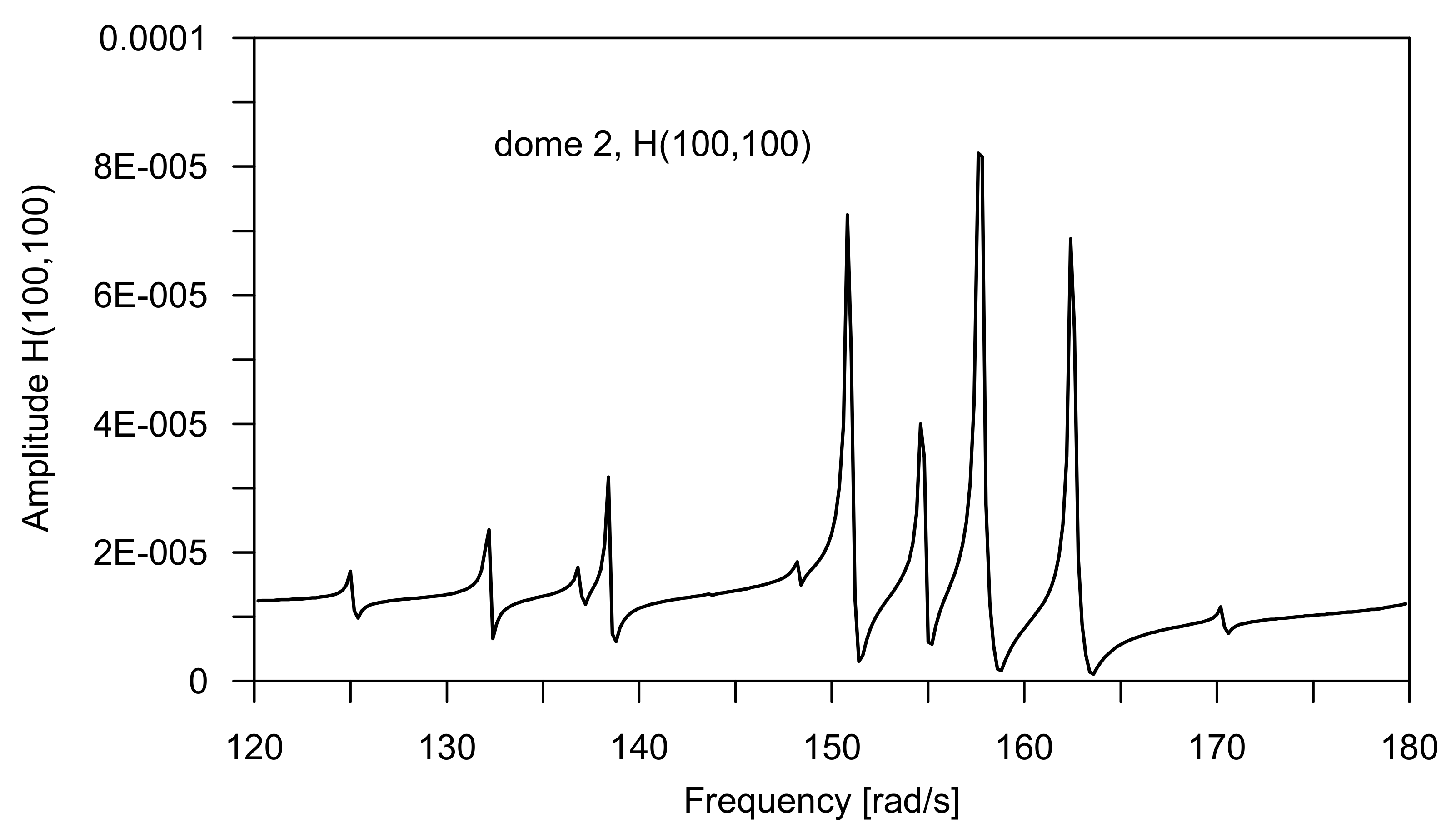
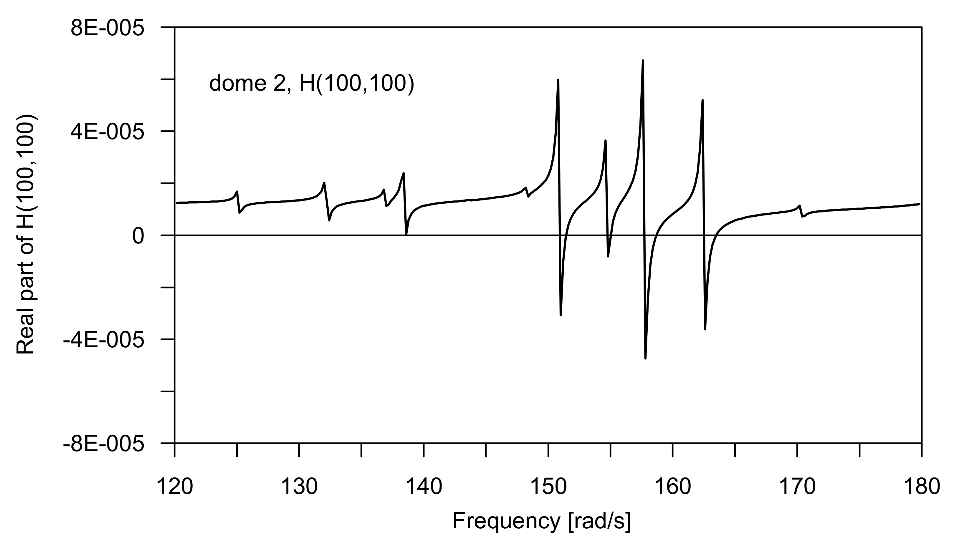
Besides natural frequencies, damping ratios and modes of vibration, the FRFs are also important dynamic characteristics of each structure. When FRFs are of interest, the excitation forces are assumed to be in the form

$$P(t)={\overline{P}}_1{e}^{\mathrm{i}\lambda t},$$

(58)

and the solution to Equation (56) could be written as

$${\overline{q}}_1=H(\lambda ){\overline{P}}_1,$$

(59)

where

$$H(\lambda )={[K_s+{\theta }_1(\tau \lambda )K_v-{\lambda }^{2}M]}^{-1}$$

(60)

is the searched matrix of FRF.

Element $H_{ij}(\lambda )$ of the matrix FRF is the displacement of the i-th degree of freedom of the structure at hand, subjected to the unit’s harmonically varying force at the j-th degree of freedom.

5. Results of Representative Calculation

5.1. General Information Concerning the Numerical Algorithm

The considered problem required a solution to NEP (31) when the natural frequencies, the non-dimensional damping ratios and the modes of vibration are of interest. The FRFs are determined after using formula (60) for a set of excitation frequencies, $\lambda$. At the beginning of the numerical procedure, the global system matrices $M$, $K_s$ and $K_v$ must be calculated. These matrices are calculated manually (in the case of Example 1) or using the commercial program Abaqus (in Example 2).

The finite element, called EB32, is used to generate all the above-mentioned matrices by Abaqus. Still, a special method of calculation is required because all the above-mentioned matrices are a sum of the matrices that take into account the influence of the elastic and the VE parts of the rods. In fact, when calculating the above-mentioned matrices, three fictitious elastic structures are defined. The first artificial structure has purely elastic rods, the elastic modulus of which is $E_s$, and the cross-sections are identical with the cross-sections of the elastic part of the real structures. The second artificial structure is also purely elastic, but its rod’s cross-sections are identical with the VE parts of the rod’s cross-sections for the real dome. The elastic modulus of the rods of the structure is $E_0$. The sum of the global mass matrices of two of the above-mentioned artificial structures gives us the global mass matrix $M$. Moreover, the sum of stiffness matrices is the global stiffness matrix $K_s$. The third artificial structure is identical with the second one, but now the elastic modulus of the rods is $\Delta E=E_{\infty }-E_0$ instead of $E_0$. The matrix $K_v$ is the stiffness matrix of the third artificial dome.

The program for solving NEP and the program for calculating FRFs were written by the authors in Fortran, based on the theory presented in the previous sections.

5.2. Example 1—Three-Degrees-of-Freedom System

The aim of Example 1 is to validate our program for solving NEP. The considered system is shown in Figure 3 and defined by the following system matrices and vector $\overline{q}={[{\overline{q}}_1,{\overline{q}}_2,{\overline{q}}_3]}^T$:

$$M=\left[\begin{array}{lll}100.0& 0.0& 0.0\\ 0.0& 100.0& 0.0\\ 0.0& 0.0& 100.0\end{array}\right] [kg], K_s=K_v={10}^5\left[\begin{array}{lll}4.0& -2.0& 0.0\\ -2.0& 4.0& -2.0\\ 0.0& -2.0& 4.0\end{array}\right] [N/m].$$

The VE part of the system at hand is modeled using the fractional Zener model with the following parameters: $\tau =0.04 \mathrm{ms}$, $\alpha =0.8$ and $E_{\infty }=2E_0$, which means that $\Delta E/E_0=1$. The natural frequencies of the system, treated as being purely elastic, are: ${\omega }_1=10.8239 rad/s$, ${\omega }_2=20.0 rad/s$ and ${\omega }_3=26.1313 rad/s$. Using the continuation method described in Section 3, the following results are obtained:

$$s_1=-1.70018\pm 12.3912, s_2=-3.28087\pm 24.7052, s_3=-4.03237\pm 33.2466.$$

In fact, the considered system is the one with proportional damping. It was discussed in detail in [40], and, for this type of system, it is enough to solve the following nonlinear algebraic equation

$$s^2+{\omega }^2\left(1+\theta (s)\frac{\Delta E}{E_0}\right)=0 ,$$

(61)

instead of solving NEP (31). In (61), $\omega$ is the natural frequency of the corresponding elastic system. By solving (61) with respect to $s$ and using the above natural frequencies of the elastic system, we obtain

$$s_1=-1.70055\pm 12.3912, s_2=-3.28079\pm 24.7053, s_2=-4.03226\pm 33.2467.$$

It is easy to note that the results obtained by both methods are almost identical. The natural frequencies and the non-dimensional damping ratios are:

$${\omega }_1=12.5073 rad/s, {\omega }_2=24.9222 rad/s, {\omega }_3=33.4903 rad/s,$$

$${\gamma }_1=0.1360, {\gamma }_2=0.1316, {\gamma }_3=0.1204.$$

It can be seen that, in this example, a system with strong damping is considered.

The modes of vibrations of the elastic and the VE systems are identical, as proved in [40].

5.3. Example 2—Small Reticulated Dome

In this example, the reticulated dome shown in Figure 4 is considered. The coordinates of the dome’s nodes are collected in

Table 1. Coordinates of the dome’s nodes (cm).

Node	x	y	z	Node	x	y	z
1	0	0	64.728	8	346.410	200.0	0
2	200.0	0	49.728	9	0	400.0	0
3	100.0	173.205	49.728	10	−346.410	200.0	0
4	−100.0	173.205	49.728	11	−346.410	−200.0	0
5	−200.0	0	49.728	12	0	−400.0	0
6	−100.0	−173.205	49.728	13	346.410	−200.0	0
7	100.0	−173.205	49.728	-	-	-	-

. All the rods have identical physical properties (except length). The elastic part of the rod is in the shape of a pipe, the external radius of which is $R=2.50 \mathrm{cm}$, and its wall thickness is $d_s=0.50 \mathrm{cm}$. The mechanical parameters of the elastic part of the rod are: material density ${\rho }_s=7782.0{ \mathrm{kg}/\mathrm{m}}^3$, elastic modulus $E_s=176.24 \mathrm{GPa}$, shear modulus $G_s=67.785 \mathrm{GPa}$, Poisson’s ratio $\nu =0.3$.

Four versions of a rod are presented in Figure 5, where the cross-section of a typical rod is shown. In the first version, the rod is purely elastic. In the second version, the VE layer is glued to the outer wall of the pipe and has a thickness $d_{\nu }=0.60 \mathrm{cm}$. In the third version, the VE layer is glued to the inner wall of the pipe and also has a thickness $d_{\nu }=0.60 \mathrm{cm}$. In the fourth version, the inside of the pipe is filled with the VE material which is glued to the elastic part of the rod.

The parameters of the Zener model are taken from [61]. The values of the model parameters are: ${\rho }_{\nu }=1423.0{ \mathrm{kg}/\mathrm{m}}^3$, $E_0=0.353 \mathrm{GPa}$, $E_{\infty }=3.462 \mathrm{GPa}$, $G_0=0.136 \mathrm{GPa}$, $G_{\infty }=0.470 \mathrm{GPa}$, $\tau =0.0003149 \mathrm{s}$, $\alpha =0.873$ and $\nu =0.3$.

The tenth natural frequencies of the domes are collected in

Table 2. Natural frequencies of domes with different cross-sections (rad/s).

Mode	Dome 1	Dome 2	Dome 3	Dome 4
1	138.135	122.702	128.007	120.095
2	146.069	129.738	135.365	127.009
3	146.069	129.738	135.365	127.009
4	151.374	134.445	140.283	131.627
5	153.017	135.905	141.806	133.055
6	153.017	135.906	141.806	133.055
7	158.608	140.893	146.976	137.889
8	163.660	145.380	151.658	142.282
9	163.660	145.380	151.658	142.282
10	166.872	148.187	154.658	145.131

. In calculating these frequencies, each dome is treated as a purely elastic system with the moduli $E_s$, $G_s$ and $E_0$, $G_0$ for a real elastic part of the dome and taking into account only the relaxed elastic moduli of the VE part of the dome, respectively. Two versions of the initial approximation of NEP’s solutions are tested. In the first version, the frequencies presented in Table 2 are used as a starting value of the eigenvalue $s$, as given in (38). The corresponding linear mode of vibration is chosen as the starting approximation of the nonlinear eigenvector. It can be seen that the VE part of the domes significantly changes natural frequencies in comparison with the dome without the VE part. Moreover, it could be observed that natural frequencies of the domes are not well separated, and there are three pairs of double natural frequencies for each dome. In the second version, the natural frequencies and modes of vibration of dome 1 are chosen as the initial approximation of the NEP’s solution.

The first five eigenvalues obtained as the solutions to NEP are presented in

Table 3. Dome 2—NEP eigenvalues, natural frequency, non-dimensional damping ratio and MAC.

Mode	$\mathit{s}$	$\mathit{\omega }$ [rad/s]	$\mathit{\gamma }$ [-]	${\mathit{\gamma }}_{\mathit{M}\mathit{S}\mathit{M}}$ [-]	MAC
1	−0.1388584 + i 122.738	122.738	0.0011313	0.0012497	1.000
2	−0.146917 + i 129.777	129.777	0.0011321	0.0011314	0.931
3	−0.146917 + i 129.777	129.777	0.0011321	0.0011314	0.931
4	−0.154446 + i 134.486	134.486	0.0011485	0.0011478	1.000
5	−0.157751 + i 135.947	135.947	0.0011604	0.0011597	0.986

,

Table 4. Dome 3—NEP eigenvalues, natural frequency, non-dimensional damping ratio and MAC.

Mode	$\mathit{s}$	$\mathit{\omega }$ [rad/s]	$\mathit{\gamma }$ [-]	${\mathit{\gamma }}_{\mathit{M}\mathit{S}\mathit{M}}$ [-]	MAC
1	−0.033814 + i 128.016	128.016	0.0002641	0.0002641	1.000
2	−0.041082 + i 135.376	135.376	0.0003035	0.0003034	0.997
3	−0.041082 + i 135.376	135.376	0.0003035	0.0003034	0.997
4	−0.045141 + i 140.295	140.295	0.0003218	0.0003217	1.000
5	−0.045945 + i 141.818	141.818	0.0003240	0.0003239	0.980

and

Table 5. Dome 4—NEP eigenvalues, natural frequency, non-dimensional damping ratio and MAC.

Mode	$\mathit{s}$	$\mathit{\omega }$ [rad/s]	$\mathit{\gamma }$ [-]	${\mathit{\gamma }}_{\mathit{M}\mathit{S}\mathit{M}}$ [-]	MAC
1	−0.041029 + i 120.106	120.106	0.0003416	0.0003416	1.000
2	−0.054347 + i 127.023	127.023	0.0004278	0.0004278	0.981
3	−0.054347 + i 127.024	127.024	0.0004278	0.0004278	0.981
4	−0.061145 + i 131.643	131.643	0.0004645	0.0004644	1.000
5	−0.062149 + i 133.071	133.071	0.0004670	0.0004670	0.999

for domes 2, 3 and 4 (i.e., domes with the VE part). These results are obtained using the classical continuation method and with the help of the method suggested by Jarlebring et al. All results are identical. Moreover, the corresponding natural frequencies $\omega$ and the non-dimensional damping ratios $\gamma$ are shown in the Tables. The non-dimensional damping ratios are also calculated by means of the modal strain method and are denoted in Table 3, Table 4 and Table 5 as ${\gamma }_{MSM}$. Appendix E gives us the appropriate formulae. It can be seen for all the domes that two solutions to NEP (the second and the third ones are identical) give us identical eigenvalues. Moreover, the obtained natural frequencies for the domes with the VE part are almost identical with the starting approximation of the eigenvalues shown in Table 2, Columns 3, 4 and 5. However, the above-mentioned natural frequencies are not close to the natural frequencies of a purely elastic dome (dome 1). The non-dimensional damping ratios obtained as the solutions to NEP are very similar to those determined with the help of the modal strain method. For dome 2, the non-dimensional damping ratios are higher. In general, the considered domes are slightly damped systems.

In Table 3, Table 4 and Table 5, the abbreviation MAC means the modal assurance criterion, applied to two complex vectors, $q_i$ and $q_j$. MAC is defined as follows (see [62,63]):

$$\mathrm{MAC}=\frac{({\overline{q}}_i^H{q}_j)}{({\overline{q}}_i^H{q}_i)({\overline{q}}_j^H{q}_j)},$$

(62)

where the bar over the quantity means that it is a complex conjugate to the same quantity without the bar. The values of MAC approximately equal to one mean that both vectors are similar, whereas the values of MAC approximately equal to zero mean that the vectors are very different and nearly orthogonal. The above criterion is used to compare the linear mode of vibration, adopted as the starting approximation of NEP’s eigenvectors with the eigenvectors obtained as the solution to NEP. When examining the values of MAC in Table 3, Table 4 and Table 5, it can be concluded that nonlinear eigenvectors (complex mode of vibration) are very similar to the modes of vibration of the elastic dome 1.

In order to make the presentation of the numerical analysis more complete, the first three nonlinear eigenvectors obtained as NEP solutions for dome 2 are presented in Figure 6, Figure 7, Figure 8, Figure 9, Figure 10 and Figure 11. The first eigenvector is shown in Figure 6 (where the real part of the eigenvector is visible) and in Figure 7 (where its imaginary part is presented). The values of the imaginary part of the eigenvector are multiplied by 1500 in order to make this part of the eigenvector visible in contrast to the real part of the eigenvector. In a similar way, the second eigenvector (in Figure 8 and Figure 9) and the third eigenvector (in Figure 10 and Figure 11) are shown. It should be noted that the second and third eigenvectors correspond to natural frequencies, which are equal. It is easy to see that the second and third eigenvectors have different shapes, but symmetries in the shapes of all three eigenvectors are visible. As was concluded previously, the presented nonlinear eigenvectors are very similar to the linear modes of vibration.

With the exception of the first incremental step of the continuation procedure, in a typical incremental step, one or two iterations are required to achieve a convergent solution to NEP for the given value of the continuation parameter $\kappa$. However, in the first incremental step, a number of iterations are likely to be of the order 10 when the Jarlebring method is used. This fact suggests that the proposed initial approximation of the solution is not optimal. The second choice of the above-mentioned initial approximation of the NEP’s solution is assumed as the natural frequency and mode of vibration of dome 1, i.e., the dome built of the elastic material only. The obtained solution to NEP is identical to that in the previous cases, but the number of iterations in the initial increment is drastically smaller (not greater than 4). Moreover, in all cases, the value of MAC is equal to 1 or very near to 1, which means that nonlinear eigenvectors are very similar to the modes of vibration of the elastic dome (dome 1). The presented results illustrate the influence of the initial approximation of the NEP’s solution on the speed of convergence of the computational procedure.

The effect of the thickness of the VE layer is illustrated in

Table 6. Dome 2—NEP eigenvalues, natural frequency, non-dimensional damping ratio and MAC—the 1.0 cm-thick VE layer.

Mode	$\mathit{s}$	$\mathit{\omega }$ [rad/s]	$\mathit{\gamma }$ [-]	${\mathit{\gamma }}_{\mathit{M}\mathit{S}\mathit{M}}$ [-]	MAC
1	−0.041527 + i 117.829	117.829	0.0003524	0.0004032	1.000
2	−0.043391 + i 124.507	124.507	0.0003485	0.0003613	0.932
3	−0.043391 + i 124.507	124.507	0.0003485	0.0003613	0.932
4	−0.045434 + i 128.998	128.998	0.0003522	0.0003653	1.000
5	−0.046394 + i 130.401	130.401	0.00035578	0.0003692	0.986

, where the results of calculation for dome 2, with a 1.0 cm-thick layer, are presented. When comparing the results in Table 3 and Table 6, it can be seen that the non-dimensional damping ratios for dome 2 with a thicker VE layer are much lower. Moreover, the natural frequencies are also lower.

At the end of the discussion of the results of the numerical analysis, the dynamic characteristics of dome 2 are presented again, but for different parameters of the VE material. The parameter values are taken from [64], where they are presented in Table 2 and are described as a polymer that exhibits high damping. However, a different rheological model was used to describe the Zener model; therefore, the values presented in [64] cannot be used directly and must be used to calculate the parameters of the model adopted here. This is carried out under the assumption that the maximal material loss factor appears for $\omega =150 \mathrm{rad}/\mathrm{s}$. In the end, the following values of model parameters are obtained: $E_0=1.0 \mathrm{GPa}$, $E_{\infty }=1.5 \mathrm{GPa}$, $G_0=0.384 \mathrm{GPa}$, $G_{\infty }=0.577 \mathrm{GPa}$, $\nu =0.3$, $\tau =0.0486 \mathrm{s}$, $\alpha =1.0$, ${\rho }_v=1200.0{ \mathrm{kg}/\mathrm{m}}^3$.

The first five solutions of NEP, together with their corresponding natural frequencies and non-dimensional damping ratios, are presented in

Table 7. Dome 2—NEP eigenvalues, natural frequency, non-dimensional damping ratio and MAC; data taken from [64].

Mode	$\mathit{s}$	$\mathit{\omega }$ [rad/s]	$\mathit{\gamma }$ [-]	${\mathit{\gamma }}_{\mathit{M}\mathit{S}\mathit{M}}$ [-]	MAC
1	−0.064433 + i 125.739	125.739	0.00051244	0.0004684	1.000
2	−0.061676 + i 132.905	132.906	0.00046406	0.0004242	0.999
3	−0.061676 + i 132.906	132.906	0.00046406	0.0004242	0.999
4	−0.060819 + i 137.713	137.713	0.00044164	0.00040358	0.999
5	−0.060905 + i 139.210	139.210	0.00043750	0.00039990	0.999

. The classic continuation method was used to solve NEP. It is found for the new VE material that the non-dimensional damping ratios are lower in comparison with the previous case (compare Table 3). The modes of vibration and the corresponding natural frequencies of a purely elastic dome were used as the initial approximation of the NEP’s solution. The iterative procedure was very fast, and, based on the values of MAC given in Table 7, it can be concluded that all nonlinear eigenvectors are very similar to the above-mentioned modes of vibration of the elastic dome.

The frequency response functions are also calculated. Typical results are presented in Figure 12, where the amplitudes of function $H_{100,100}(\lambda )$ calculated for dome 2 and using the first set of values of the VE parameters are shown. Comparing the results in Table 3 with those presented in Figure 12, it can be seen that the first few resonance regions are in agreement with natural frequencies, calculated by the continuation method. In order to make the description of our results concerning FRF more complete, the real part of FRF is presented in Figure 13, and the imaginary part of FRF is shown in Figure 14.

6. Concluding Remarks

A method for the determination of the dynamic characteristics of reticulated domes is presented. The considered reticulated domes are built of composite rods. Each rod is composed of two parts: one is purely elastic and the other is built of a viscoelastic material. The fractional Zener model is adopted to describe the damping properties of the VE material. For a first time, the finite element for the 3D rods composed of two parts (elastic and VE) is formulated. The Timoshenko theory and the Laplace transformation are used to derive the nonlinear eigenvalue problem. The natural frequencies, the non-dimensional damping ratios and the modes of vibration of the three versions of the composed domes are obtained as the solution to NEP. The continuation method is used to solve the above-mentioned NEP very effectively. The continuation procedure is very effective: it is able to solve NEP for a system with separated and repeated natural frequencies. Moreover, the procedure for the determination of the frequency response functions is also presented. The results for representative small VE domes are presented to illustrate the proposed numerical procedure. The results of calculation are also briefly discussed. The main novelties and the results presented in the paper can be summarized as follows:

• According to our best knowledge, this is the first work that analyzes the dynamic characteristics of reticulated domes composed of rods which are built of viscoelastic and elastic parts.
• The description of the above-mentioned composite rods treated as 3D rods is also unique.
• It is proved by numerical analysis that the presented versions of the continuation method are a very effective way of solving the considered nonlinear eigenvalue problem and that they can solve it for systems with separated and repeated natural frequencies. This is important because domes are often systems with repeated natural frequencies.
• The presented results of the numerical analysis suggest that the types of domes considered here are slightly damped. An extended numerical analysis of other domes (larger and different types) is very desirable.

References

1. Kelly, J.M. Aseismic base isolation: Review and bibliography. Soil Dynam. Earthq. Eng. 1986, 5, 202–216. [Google Scholar] [CrossRef]
2. Lewandowski, R. Reduction of Vibration of Building Structures, 1st ed.; PWN: Warsaw, Poland, 2014. (In Polish) [Google Scholar]
3. De Domenico, D.; Ricciardi, G.; Takewaki, I. Design strategies of viscous dampers for seismic protection of building structures: A review. Soil Dynam. Earthq. Eng. 2019, 118, 144–165. [Google Scholar] [CrossRef]
4. Pawlak, Z.; Lewandowski, R. The continuation method for the eigenvalue problem of structures with viscoelastic dampers. Comput. Struct. 2013, 125, 53–61. [Google Scholar] [CrossRef]
5. Spencer, B.F.; Nagarajaiah, S. State of the art of structural control. J. Struct. Eng. 2003, 129, 845–856. [Google Scholar] [CrossRef]
6. Kato, S.; Ueki, T.; Mukaiyama, Y. Study of dynamic collapse of single layer reticular domes subjected to earthquake motion and estimation of statically equivalent seismic force. Int. J. Space Struct. 1997, 12, 191–203. [Google Scholar] [CrossRef]
7. Ishikawa, K.; Kato, S. Elastic-plastic dynamic buckling analysis of reticular domes subjected to earthquake motion. Int. J. Space Struct. 1997, 12, 205–215. [Google Scholar] [CrossRef]
8. Nie, G.B.; Zhi, X.D.; Fan, F.; Dai, J.W. Seismic performance evaluation of single-layer reticulated dome and its fragility analysis. J. Constr. Steel Res. 2014, 100, 176–182. [Google Scholar]
9. Zhang, H.D.; Han, Q.H. A numerical investigation of seismic performance of large span single-layer latticed domes with semi-rigid joints. Struct. Eng. Mech. 2013, 48, 57–75. [Google Scholar] [CrossRef]
10. Li, Q.S.; Chen, J.M. Nonlinear elastoplastic dynamic analysis of single-layer reticulated shells subjected to earthquake excitation. Comput. Struct. 2003, 81, 177–188. [Google Scholar] [CrossRef]
11. Zhi, X.; Fan, F.; Shen, S. Elasto-plastic instability of single-layer reticulated shells under dynamic actions. Thin-Walled Struct. 2010, 48, 837–845. [Google Scholar] [CrossRef]
12. Yin, Y.; Huang, X.; Han, Q.; Bai, L. Study on the accuracy of response spectrum method for long-span reticulated shells. Int. J. Space Struct. 2009, 24, 27–35. [Google Scholar] [CrossRef]
13. Wu, Y.; Zhang, J.S.; Chen, B.; Shen, S.Z. Identification of the dominant vibration modes of single-layer reticulated shells under wind action. Int. J. Space Struct. 2007, 22, 123–132. [Google Scholar] [CrossRef]
14. Li, Z.; Zuyan, S. Shaking table test of two shallow reticulated shells. Int. J. Solids Struct. 2001, 38, 7875–7884. [Google Scholar]
15. Zhang, C.X.; Nie, G.B.; Dai, J.W.; Zhi, X.D. Experimental studies of the seismic behaviour of double-layer lattice space structures I: Experimental verification. Eng. Fail. Anal. 2016, 64, 85–96. [Google Scholar] [CrossRef]
16. Yang, F.; Zhi, X.; Fan, F. Effect of complex damping on seismic responses of a reticulated dome and shaking table test validation. Thin-Walled Struct. 2019, 134, 407–418. [Google Scholar] [CrossRef]
17. Zhang, H.D.; Wang, Y.F.; Han, Q.H. Nonlinear material loss factors of single-layer latticed domes subjected to earthquake ground motions. J. Struct. Eng. 2015, 141, 0401418. [Google Scholar] [CrossRef]
18. Zhang, H.; Han, Q.; Wang, Y.; Lu, Y. Explicit modeling of damping of a single-layer latticed dome with an isolation system subjected to earthquake ground motions. Eng. Struct. 2016, 106, 154–165. [Google Scholar] [CrossRef]
19. Xu, Z.D.; Huang, X.H.; Lu, L.H. Experimental study on horizontal performance of multi-dimensional high-damping earthquake isolation devices for long-span reticulate structures. J. Vibr. Control 2012, 18, 941–952. [Google Scholar] [CrossRef]
20. Lu, Y.; Hao, G.; Han, Q.; Huang, J. Steel tubular friction damper and vibration reduction effects, of double-layer reticulated shells. J. Constr. Steel Res. 2020, 169, 106019. [Google Scholar] [CrossRef]
21. Nie, G.; Li, D.; Zhi, X.; Chen, Q.; Wang, F. Three-dimensional seismic isolation study of single-layer reticulated domes by parameter analysis. Int. J. Steel Struct. 2021, 21, 1953–1965. [Google Scholar] [CrossRef]
22. Han, Q.; Guo, F.; Liu, M.; Lu, Y. Experimental study on the mechanical properties of a multi-dimensional vibration control damper. J. Constr. Steel Res 2022, 197, 107500. [Google Scholar] [CrossRef]
23. Dede, T.; Grzywiński, M.; Selejdak, J. Continuous size optimization of large-scale dome structures with dynamic constraints. Struct. Eng. Mech. 2020, 73, 397–405. [Google Scholar] [CrossRef]
24. Li, L.J.; Xie, Z.H.; Guo, Y.C.; Liu, F. Structural optimization and dynamic analysis for double-layer spherical reticulated shell structures. J. Constr. Steel Res. 2006, 62, 943–949. [Google Scholar] [CrossRef]
25. Ma, H.H.; Shan, Z.W.; Fan, F. Dynamic behaviour and seismic design method of a single-layer reticulated shell with semi-rigid joints. Thin-Walled Struct. 2017, 119, 544–557. [Google Scholar] [CrossRef]
26. Zhang, H.; Zhu, X.; Yao, S. Nonlinear dynamic analysis method for large-scale single-layer lattice domes with uncertain-but-bounded parameters. Eng. Struct. 2020, 203, 109780. [Google Scholar] [CrossRef]
27. Zhang, H.; An, N.; Zhu, X. Structural dynamic reliability analysis of super large-scale lattice domes during earthquakes using the stochastic finite element method. Soil Dynam. Earthq. Eng. 2022, 153, 107076. [Google Scholar] [CrossRef]
28. Xu, Z.D.; Wang, S.A.; Xu, C. Experimental and numerical study on long-span reticulate structure with multidimensional high-damping earthquake isolation devices. J. Sound Vib. 2014, 333, 3044–3057. [Google Scholar] [CrossRef]
29. Zhang, H.; Liu, X.; Li, H.; An, N. A comparative study on the effectiveness of bidirectional and tridirectional isolation systems used in large-scale single-layer lattice domes during earthquakes. Soil Dynam. Earthq. Eng. 2021, 141, 106488. [Google Scholar] [CrossRef]
30. Xu, Z.D.; Tu, Q.; Guo, Y.F. Experimental study on vertical performance of multidimensional earthquake isolation and mitigation devices for long-span reticulated structures. J. Vibr. Control 2012, 18, 1971–1985. [Google Scholar] [CrossRef]
31. Zhou, Z.; Meng, S.; Wu, J.; Zhao, Y. Semi-active control on long-span reticulated steel structures using MR dampers under multi-dimensional earthquake excitations. Smart Struct. Syst. 2012, 10, 557–572. [Google Scholar] [CrossRef]
32. Xu, J.; Xu, S.; Yuan, Z. Probabilistic seismic analysis of single-layer reticulated shell structures controlled by viscoelastic dampers with an effective placement. Eng. Struct. 2020, 222, 111052. [Google Scholar] [CrossRef]
33. Fan, F.; Shen, S.Z.; Parke, G.A.R. Theoretical and experimental study of vibration reduction in braced domes using a viscous damper system. Int. J. Space Struct. 2004, 19, 195–202. [Google Scholar] [CrossRef]
34. Yang, Y.; Spencer, B.F.; Li, Y.; Shen, S. Seismic performance of double-layer spherical reticulated shell with replaceable bar-type dampers. Int. J. Space Struct. 2011, 26, 31–44. [Google Scholar] [CrossRef]
35. Nie, G.; Liu, K. Experimental Studies of Single-Layer Reticulated Domes with Isolated Supports. Shock Vibr. 2018, 6041878. [Google Scholar] [CrossRef]
36. Yang, Y.; Hui, M. Optimal topology design of replaceable bar dampers of a reticulated shell based on sensitivity analysis. Earthq. Eng. Eng. Vib. 2014, 13, 113–124. [Google Scholar] [CrossRef]
37. Zhong, J.; Zhang, J.; Zhi, X.; Fan, F. Identification of dominant modes of single-layer reticulated shells under seismic excitations. Thin-Walled Struct. 2018, 127, 676–687. [Google Scholar] [CrossRef]
38. Horr, A.M.; Schmidt, L.C. Frequency domain dynamic analysis of large space structure with added elastomeric damper. Int. J. Space Struct. 1996, 11, 279–289. [Google Scholar] [CrossRef]
39. Horr, A.M.; Schmidt, L.C. A fractional-spectral method for vibration of damped space structures. Eng. Struct. 1996, 18, 947–956. [Google Scholar] [CrossRef]
40. Lewandowski, R.; Wielentejczyk, P. Analysis of dynamic characteristics of viscoelastic frame structures. Arch. Appl. Mech. 2020, 90, 147–171. [Google Scholar] [CrossRef] [Green Version]
41. Teng, T.L.; Hu, N.K. Analysis of damping characteristics for viscoelastic laminated beams. Comput. Meth. Appl. Mech. Eng. 2001, 190, 3881–3892. [Google Scholar] [CrossRef]
42. Cortés, F.; Sarría, I. Dynamic analysis of three-layer sandwich beams with thick viscoelastic damping core for finite element applications. Shock Vibr. 2015, 2015, 736256. [Google Scholar] [CrossRef] [Green Version]
43. Luo, Y. An efficient 3D Timoshenko beam element with consistent shape functions. Adv. Theor. Appl. Mech. 2008, 1, 95–106. [Google Scholar]
44. Voss, H. Nonlinear eigenvalue problems. In Handbook of Linear Algebra 164; Chapman and Hall/CRC: Boca Raton, FL, USA, 2003. [Google Scholar]
45. Mehrmann, V.; Voss, H. Nonlinear eigenvalue problem: A challenge for modern eigenvalue methods. Mitt. Ges. Für Angew. Math. Und Mech. GAMM-Mitt 2004, 27, 121–152. [Google Scholar] [CrossRef]
46. Güttel, S.; Tisseur, F. The nonlinear eigenvalue problem. Acta Numer. 2017, 26, 1–94. [Google Scholar] [CrossRef] [Green Version]
47. Ruhe, A. Algorithms for the nonlinear eigenvalue problem. SIAM J. Numer. Anal. 1973, 10, 674–689. [Google Scholar] [CrossRef]
48. Singh, K.V. Eigenvalue and eigenvector computation for discrete and continuous structures composed of viscoelastic materials. Int. J. Mech. Sci. 2016, 110, 127–137. [Google Scholar] [CrossRef]
49. Daya, E.M.; Azrar, L.; Potier-Ferry, M. An amplitude equation for the non-linear vibration of viscoelastically damped sandwich beams. J. Sound Vib. 2004, 271, 789–813. [Google Scholar] [CrossRef]
50. Lewandowski, R.; Baum, M. Dynamic characteristics of multilayered beams with viscoelastic layers described by the fractional Zener model. Arch. Appl. Mech. 2015, 85, 1793–1814. [Google Scholar] [CrossRef]
51. Wielentejczyk, P.; Lewandowski, R. Geometrically nonlinear, steady state vibration of viscoelastic beams. Int. J. Non-Lin. Mech. 2017, 89, 177–186. [Google Scholar] [CrossRef]
52. Lewandowski, R. Influence of temperature on the dynamic characteristics of structures with viscoelastic dampers. J. Struct. Eng. 2019, 145, 04018245. [Google Scholar] [CrossRef]
53. Mentrasti, L. Exact deflation in the complex modal analysis of low-rank nonclassically damped structures. Eng. Struct. 2012, 45, 496–508. [Google Scholar] [CrossRef]
54. Chen, X.; Chen, H.L.; Hu, X.L. Damping prediction of sandwich structures by order reduction- iteration approach. J. Sound Vib. 1999, 222, 803–812. [Google Scholar] [CrossRef]
55. Duigou, L.; Mostafa Daya, E.l.; Potier-Ferry, M. Iterative algorithms for non-linear eigenvalue problems. Application to vibrations of viscoelastic shells. Comput. Meth. Appl. Mech. Eng. 2003, 192, 1323–1335. [Google Scholar] [CrossRef]
56. Lin, R.M.; Ng, T.Y. An iterative method for exact eigenvalues and eigenvectors of general nonviscously damped structural systems. Eng. Struct. 2019, 180, 630–641. [Google Scholar] [CrossRef]
57. Leung, A.Y.T. Subspace iteration for complex symmetric eigenproblems. J. Sound Vib. 1995, 184, 627–637. [Google Scholar] [CrossRef]
58. Łasecka–Plura, M.; Lewandowski, R. The subspace iteration method for nonlinear eigenvalue problems occurring in dynamics of structures with viscoelastic elements. Comp. Struct. 2021, 254, 106571. [Google Scholar] [CrossRef]
59. Jarlebring, E.; Koskela, A.; Mele, G. Disguised and new quasi-Newton methods for nonlinear eigenvalue problems. Numer. Algorithms 2018, 79, 311–335. [Google Scholar] [CrossRef] [Green Version]
60. Litewka, P.; Lewandowski, R.; Wielentejczyk, P. Free vibrations of laminate plates with viscoelastic layers using the refined zig-zag theory—Part 2. Numerical analysis. Composite Struct. 2021, 278, 114550. [Google Scholar] [CrossRef]
61. Zarraga, O.; Sarría, I.; García-Barruetabeña, J.; Cortés, F. Dynamic analysis of plates with thick unconstrained layer damping. Eng. Struct. 2019, 201, 109809. [Google Scholar] [CrossRef]
62. Pastor, M.; Binda, M.; Harcarik, T. Modal assurance criterion. Procedia Eng. 2012, 48, 543–548. [Google Scholar] [CrossRef]
63. Cortes, F.; Elejabarrieta, M.J. An approximate numerical method for the complex eigenproblem in systems characterised by a structural damping matrix. J. Sound Vibr. 2006, 296, 166–182. [Google Scholar] [CrossRef]
64. Wehmeyer, S.C.; Compton, B.G.; Pro, J.W.; Zok, F.; Begley, M.R. Damping in cellular structures made from composite struts and walls with elastic and viscoelastic phases. J. Mech. Phys. Solids 2020, 145, 104106. [Google Scholar] [CrossRef]
65. Lee, D.G.; Hong, S.; Kim, J. Efficient seismic analysis of building structures with added viscoelastic dampers. Eng. Struct. 2002, 24, 1217–1227. [Google Scholar] [CrossRef]
66. Sun, B.; Wang, J.; Li, Z.; Qin, Y.; Liu, S.; Tomker, D. Modified modal strain energy method for analyzing the dynamic damping behavior of constrained viscoelastic structures. J. Eng. Sci. Techn. Rev. 2017, 10, 174–180. [Google Scholar] [CrossRef]
Figure 1. The possible cross-sections of composite VE rods; the grey area is VE.
Buildings 12 01999 g001
Figure 2. The two-node finite element of the rod in three dimensions.
Buildings 12 01999 g002
Figure 3. Three-degrees-of-freedom VE system.
Buildings 12 01999 g003
Figure 4. The reticulated dome.
Buildings 12 01999 g004
Figure 5. Versions of the considered cross-section of the rod. (a) the cross-section of rod - dome 1; (b) the cross-section of rod - dome 2; (c) the cross-section of rod - dome 3; (d) the cross-section of rod – dome 4 LR.
Buildings 12 01999 g005
Figure 6. Dome 2—real part of the first nonlinear eigenvector.
Buildings 12 01999 g006
Figure 7. Dome 2—imaginary part of the first nonlinear eigenvector (values multiplied by 1500).
Buildings 12 01999 g007
Figure 8. Dome 2—real part of the second nonlinear eigenvector.
Buildings 12 01999 g008
Figure 9. Dome 2—imaginary part of the second nonlinear eigenvector (values multiplied by 1500).
Buildings 12 01999 g009
Figure 10. Dome 2—real part of the third nonlinear eigenvector.
Buildings 12 01999 g010
Figure 11. Dome 2—imaginary part of the third nonlinear eigenvector (values multiplied by 1500).
Buildings 12 01999 g011
Figure 12. Representative frequency response curve.
Buildings 12 01999 g012
Figure 13. Real part of the representative frequency response curve.
Buildings 12 01999 g013
Figure 14. Imaginary part of the representative frequency response curve.
Buildings 12 01999 g014