A Numerical Method for Solving Global Irradiance on the Facades of Building Stocks

Abstract

Due to the influence of surrounding buildings on the radiation transfer process, the irradiance of individual buildings in building stocks is more uneven and different than that of individual buildings in open spaces. In view of the defect of the existing building surface irradiance calculation model in the sky radiation energy balance calculation, the complex surface reflection radiative transfer in diffuse irradiance, and complex processes, this paper combined the calculation of the complex surface narrow sky view, multiple reflections, and radiation characteristics of nonuniformity, and finally established the model for irradiance on the facade of a building stock (IFBS model) in a sheltered environment. The simulation results show that the IFBS model is superior to the traditional model in the calculation of sky diffuse irradiance and reflection irradiance of building stocks and is more suitable for the numerical calculation of the radiation transfer process of complex buildings.

1. Introduction

Radiation environment simulation is an important part of the performance simulation of the building complex. A building group performance simulation is generally attached to the third party building performance simulation module (e.g., BREDEM, EnergyPlus, DOE2). In the early days, due to the complexity of modeling and the calculation of single buildings, in order to reduce the demand for computing resources, scholars would first classify buildings into groups and then complete the calculation from single buildings to building groups by simply multiplying the number of similar buildings [1,2]. With the improvement of classification methods, scholars further classified similar buildings and made batch calculations, based on building shape [3,4], thermal parameters [5], building category [6,7] and other parameters. Although the classification processing can retain the thermal characteristics and other characteristic information of individual buildings, to a certain extent, the classification process itself is still the average processing of individual building information, so there is bound to be potential error when falling into the parameters of specific individual buildings. Along with the development of computer hardware and software, some scholars no longer categorize to simplify, but directly to each monomer building to simulate the whole compound, as per the obtained information. However, as a result of the third party building performance simulation module that is based on the monomer building performance simulation method, the impact of the surrounding buildings on the simulation of the target monomer building’s outdoor thermal environment, is relatively lacking. Therefore, there are problems, such as data distortion and data interface accuracy mismatch in the input of boundary conditions (meteorological files, etc.). For example, in EnergyPlus, only one weather file can be input to a wall. The EnergyPlus framework cannot handle different boundary conditions on the same wall, which is particularly common in buildings. Due to the limitations of tools and methods, traditional building complex simulation methods will inevitably simplify or ignore the influence of surrounding building complexes on the outdoor thermal environment of individual buildings (such as the differences in radiant heat boundary conditions, local wind environment, etc.), thus losing some details of the radiant heat process description of building complexes.

Table 1. Comparison of the methodology of existing buildings simulation models or software.

Model or Software *	Reflection Irradiance	Sky Diffuse Irradiance
Urban Canyon Model [11]	1 time reflection	isotropic
ENVI-met *	1 time reflection	isotropic
Town Energy Balance (TEB) [12]	Infinite reflection	isotropic
Temperature of Urban Facets in 3D (TUF-3D) [8]	Simplified multiple reflection	isotropic
Model for Urban Surface Temperature (MUST) [13]	Simplified multiple reflection	isotropic
DeST *	1 time reflection	isotropic
Fluent * + Solene *	1 time reflection	Perez model
TEB + EnergyPlus *	Infinite reflection	isotropic
Citysim *	1 time reflection	Perez model
INSEL * + ISO model	1 time reflection	Direct dispersion separation model
UMI *	Simplified multiple reflection	Perez model
Urban Energy Performance Calculator [14]	1 time reflection	isotropic

* Stands for software.

presents the information of the existing major simulation methods, in terms of the reflected radiation model and sky diffuse radiation models. By comparison, it can be concluded that the existing simulation methods mostly calculate the reflected radiation once. Further, the isotropic sky diffuse radiation distribution model is applied in most simulations, in order to simplify the calculation of the sky diffuse irradiance [8,9,10]. However, the accuracy of the isotropic model is acceptable under the assumption of a cloudy day or large sky view factor (SVF), which is not common in the building complex.

In the complex environment, the surrounding buildings will block the sky view field of the target building, which leads to a narrower view of the sky at the point on the surface of the target building. The narrow sky view will have an impact on the radiation transfer process of the sky diffuse radiation on the building surface, which will then have an impact on the numerical solution of the sky diffuse irradiance [15]. Sky diffuse radiation models are developed to interpret the distribution of sky diffuse radiation in the sky dome. Existing mainstream algorithms, based on the isotropic sky diffuse radiation model [16] or the Perez anisotropic sky diffuse radiation model [17,18] are under development. These two kinds of models use too many simplified assumptions, and their applicability in scenarios with a small sky view factor is limited. At the same time, it is also necessary to discuss whether the precision of the sky dome discretization needs to be improved in the current numerical calculation [19,20]. As for the reflection radiation, the current numerical method is based on Lambertian assumption and an applied finite reflection (mostly one time reflection) calculation algorithm, which leads to the heat gain of the reflected radiation being smaller [21], and the error will be significantly amplified with the increase of the building density [22].

To sum up, the study of building radiant heat processes should be based on a high-precision radiation model. The existing radiation simulation algorithms mostly follow the assumption of a single building. Therefore, there are many simplifications in the calculation of the reflection radiation and the sky diffuse radiation transfer. However, these simplifications can be adversely affected under certain conditions, especially in complex buildings. As a result, the calculation process cannot fully express the influence of building stocks on radiation transfer. The errors caused by this simplified algorithm, in calculating complex buildings and how to improve the algorithm to improve the simulation accuracy of radiation transfer processes under the influence of complex buildings remain to be studied.

In this work, a new numerical method will be constructed, based on the radiation transfer theory, and the algorithm in the solution process will be established to realize the accuracy improvement in the global irradiance simulation on the facades of building stocks. In Section 2, we analyze the radiant energy balance on the building surface, based on the net radiation analysis method. Further, we analyze the most appropriate theoretical algorithm for direct solar irradiance, sky diffuse irradiance, and reflection irradiance on the facades of building stocks. In Section 3, we develop the numerical solution of the radiation scheme. We mainly focus on the discretization of surfaces, constructing the matrix of each component of global irradiance, and obtaining a numerical equation for the global irradiance value of the building facades. In Section 4, we compare the new sky diffuse and reflection irradiance algorithm with the existing algorithm from the traditional method. The comparative analysis is based on the existing measurement study and the theoretical simulation in this work.

2. Radiation Scheme

2.1. Analysis of the Radiant Energy Balance on the Building Surface

Net radiation analysis was used to analyze the radiation energy on the surface $i$ of building facades, as shown in Figure 1.

In the figure, ${\alpha }_i,{\tau }_i,{\rho }_i$ represent the absorption rate, transmittance and reflectance of the element surface $i$, respectively, without dimensionality.

For a single element surface $i$, it can be seen from the schematic diagram of the radiation energy balance analysis, that the total irradiance received is:

$$I_{g,i}=I_{dir,i}+I_{dif,i}+I_{ref,i}$$

(1)

where $I_{dir,i},I_{dif,i},I_{ref,i},$ respectively, represent the direct solar irradiance value, sky diffuse irradiance value and the reflected irradiance from other microscopic surfaces received by surface $i$, $W/m^2$.

Meanwhile, the effective radiation (reflected radiation) intensity outward from element surface $i$ is:

$$I_{R,i}={\rho }_i{I}_{g,i}={\rho }_i\left(I_{dir,i}+I_{dif,i}+I_{ref,i}\right)$$

(2)

The reflected irradiance received by a cell surface is the cumulative value of the reflected radiation intensity from other cells:

$$I_{ref,i}={\displaystyle \sum }_{j=1}^N{I}_{R,j}{F}_{ij}$$

(3)

where $F_{ij}$ is the shape factor of the surface $i$ to the surface $j$, dimensionless. The shape factor $F_{ij}$ is defined as the fraction of energy leaving a black surface element $i$ that arrives at another black surface element $j$ [23].

To sum up, the total radiation received by a single micro-element surface $i$ can be calculated as:

$$I_{g,i}=I_{dir,i}+I_{dif,i}+{{\displaystyle \sum }}_{j=1}^N{\rho }_j{I}_{g,j}{F}_{ij}$$

(4)

2.2. Solar Direct Irradiance on the Facades of Building Stocks

2.2.1. Calculation of the Solar Orientation

In the calculation of the surface direct solar irradiance, the traditional method mainly applies the solar azimuth and solar altitude angles, which are calculated, based on latitude, declination angle, and solar hour angle, to locate the sun’s position in the sky [13,24]. In the IFBS model, the same calculation equation is used to calculate the basic parameters related to the solar azimuth, such as the solar declination angle, solar angle, altitude angle, and azimuth angle.

The calculation equation of the solar altitude angle is as follows:

$$sinh=sin\delta sin\varphi +cos\delta cos\varphi cos\omega$$

(5)

where $h$ is the solar altitude angle, $°$; $\varphi$ is the local latitude, $°$; $\omega$ is solar hour angle, $°$; $\delta$ is declination angle, $°$.

The calculation equation of the solar azimuth is:

$$cosA=\left(sinhsin\varphi -sin\delta \right)/coshcos\varphi$$

(6)

2.2.2. Judgment of Occlusion

The solar radiation obtained on any plane is related to the incidence angle of sunlight on the plane. The intensity of the direct solar irradiance, received by the surface $i$ at a fixed incidence angle can be calculated as [25]:

$$I_{dir,i}=I_{0}cos{\theta }_i$$

(7)

where $I_0$ is the direct solar radiation intensity on the surface $i$ without occlusion, $W/m^2$; ${\theta }_i$ is the solar incident angle of the micro-surface $i$, $°$.

In fact, the occlusion phenomenon is quite common in building stocks. Therefore, whether the plane is occluded, needs to be calculated. Due to the parallel characteristics of sunlight, the concept of “backward ray tracing” [26] is designed to make ray tracing more efficient. In backward ray tracing, an eye ray is created at one point; the vector direction of the ray is in the opposite direction of the sunlight. The sun will be visible from that point if the eye ray hits no object. In the backward ray tracing method, the calculation process will trace rays of interest and not consume resources tracing rays that do not contribute to the solution of the engineering/design problem. Therefore, the backward ray tracing method is wildly adopted in solar energy calculation [27,28,29] and will be applied in this paper.

Based on the above calculation of the sun’s altitude angle and azimuth, the X-axis represents the east-west direction (positive east direction), the Y-axis represents the north-south direction (positive north direction), and the Z-axis represents the altitude direction (positive upward direction). The vector of the backward ray $\stackrel{\rightharpoonup }{{\mathit{I}}_{\mathit{r}\mathit{e}\mathit{v}\mathit{,}\mathit{i}}}=\left(I_{i,x},I_{i,y},I_{i,z}\right)$ from surface $i$ at a given time

$$\left\{\begin{array}{cc}\hfill I_{i,x}=coshsinA \mathrm{if} \mathrm{solar}& \mathrm{time} \mathrm{is} \mathrm{less} \mathrm{than} 12 \mathrm{else}-coshsinA\hfill \\ & I_{i,y}=-coshcosA\hfill \\ & I_{i,z}=sinh\hfill \end{array}\right.$$

(8)

Figure 2 presents the spatial geometric relation between the backward ray and the building interface. Taking the roof’s occlusion of light as an example, let ${\alpha }_j\in V_{roof}$, where $\Delta d_j$ and $\Delta l_j$ represent the size of the roof interface ${\alpha }_j$ on Y-axis and X-axis, respectively, and $V_{roof}$ is the set of all roof interfaces. $\stackrel{\rightharpoonup }{{\mathit{I}}_{\mathit{r}\mathit{e}\mathit{v}\mathit{,}\mathit{i}}}$ represents the reverse beam vector and intersects with the plane of the roof interface ${\alpha }_j$ at the point $A_{ij}$. The geometric center of the roof interface ${\alpha }_j$ is $A_0$. Then, the judgment of the occlusion relation between the reverse beam and the roof interface ${\alpha }_j$ can be transformed into the judgment of $A_{ij}$ and $A_0$ distance. If the distance between $A_{ij}$ and $A_0$ is greater than $\Delta l_j/2$ on the X-axis or greater than $\Delta d_j/2$ on the Y-axis, it indicates that the reverse beam is not obscured by the roof interface ${\alpha }_j$.

The three-dimensional coordinates of $A_{ij}$ and $A_0$ are $\left(x_{ij},y_{ij},z_{ij}\right)$ and $\left(x_0,y_0,z_0\right),$ respectively. Then the Boolean value of the occlusion judgment between element surface $i$ and roof interface ${\alpha }_j,$ can be calculated as follows:

$$Fla{g}_{ij}=\left|x_{ij}-x_0\right|>\Delta l_j/2 | \left|y_{ij}-y_0\right|>\Delta d_j/2$$

(9)

where $Fla{g}_{ij}=1$ represents no occlusion. For all roof interfaces ${\alpha }_j\in V_{roof}$, after traversing the judgment process, it can be obtained:

$$\mathit{F}\mathit{l}\mathit{a}{\mathit{g}}_{\mathit{i}\mathbf{-}\mathit{r}\mathit{o}\mathit{o}\mathit{f}}={\left(Fla{g}_{i1},Fla{g}_{i2},\dots ,Fla{g}_{iN}\right)}^T$$

(10)

Similarly, for the set of other facades of the building, the value of $\mathit{F}\mathit{l}\mathit{a}{\mathit{g}}_{\mathit{i}-\mathit{w}\mathit{a}\mathit{l}\mathit{l}}$ can be obtained, and the calculation equation of the Boolean value of the final judgment of whether the element surface $i$ is covered is as follows:

$$Fla{g}_i=\mathit{F}\mathit{l}\mathit{a}{\mathit{g}}_{\mathit{i}\mathit{-}\mathit{r}\mathit{o}\mathit{o}\mathit{f}} \& \mathit{F}\mathit{l}\mathit{a}{\mathit{g}}_{\mathit{i}\mathit{-}\mathit{w}\mathit{a}\mathit{l}\mathit{l}}$$

(11)

where $Fla{g}_i=1$ means that the element surface $i$ is not obtained.

Finally, the equation for calculating the direct solar irradiance value on the element surface $i$ at a given time is:

$$I_{dir,i}=Fla{g}_i{I}_{dir0}cos{\theta }_i$$

(12)

where $I_{dir0}$ is the direct solar radiation intensity at this moment, $W/m^2$; ${\theta }_i$ is the solar incident angle of the micro surface $i$, $°$.

2.3. Sky Diffuse Irradiance on the Facades of Building Stocks

2.3.1. Determination of the Discrete Precision of the Sky Vault

The surface sky diffuse irradiance is obtained by integrating the product of the sky radiation intensity with the cosine of the incident angle of the sky points over all solid angles of the sky. Among them, the solid angle [30] (Figure 3) is defined as:

$$d\mathsf{\Omega }=\frac{df}{R^2}=\frac{\left(Rd\theta \right)\left(rd\varphi \right)}{R^2}$$

(13)

Assuming that the radiation intensity along the $\theta$ direction is $I_{\theta }$, the equation for calculating the sky diffuse irradiance on one surface as follows:

$$I_{dif}={{\displaystyle \int }}_0^{2\pi }{I}_{\theta }\mathit{cos}\theta d\mathsf{\Omega }={{\displaystyle \int }}_{\varphi =0}^{\varphi =2\pi }{{\displaystyle \int }}_{\theta =0}^{\theta =\frac{\pi }{2}}{I}_{\theta }\mathit{cos}\theta \mathit{sin}\theta d\varphi d\theta$$

(14)

In a non-sheltered environment, the analytical solution of the sky diffuse irradiance on the surface of the building walls can be obtained by the above equation. This method is widely used in the calculation of the surface irradiance of traditional single buildings. However, in building complexes, the shape of the visible sky area is irregular (see Figure 4), due to the narrow perspective of the sky on the surface of the buildings. Therefore, the finite element numerical method is more suitable for the calculation of the sky diffuse radiation in building complexes. The numerical method first discretizes the sky into the set of sky lattices, in which the sky diffuse radiation intensity of the micro surface $j$ along the $\theta$ direction is $I_{\theta ,sky,j}$, and then the surface sky diffuse irradiance of the plane $i$ is calculated as follows:

$$I_{dif,i}={{\displaystyle \int }}_0^{2\pi }I{F}_{\theta }{I}_{\theta ,sky,j}\mathit{cos}{\theta }_{ij}d\mathsf{\Omega }={{\displaystyle \sum }}_{j=0}^{n}I{F}_{\theta }{I}_{\theta ,sky,j}\mathit{cos}{\theta }_{ij}Are{a}_j$$

(15)

where, ${\theta }_{ij}$ is the incident angle from the micro-element surface to the plane, $°$; $I{F}_{\theta }$ is the Boolean value of the sky visible judgment along the $\theta$ direction (1 if the sky micro point is visible, 0 if it is not visible), it is dimensionless; $Are{a}_j$ is the Area of the sky element surface $j$, $m^2$; $Are{a}_j=sin\theta d\varphi d\theta$, $m^2$; $I_{\theta ,sky,j}$ is the diffuse radiation intensity at the sky micro surface $j$, $W/\left(sr·m^2\right)$.

Among the variables in Equation (15), the discrete accuracy of the sky lattice model is particularly important for the expression of the sky diffuse radiation. Existing scholars have constructed several types of sky dome partition methods, such as the Tregenza145 sky lattice model [31], which is the most widely used [32,33]. However, it is easy to have calculation errors in the calculation scenes of a narrow sky view in a building complex, due to its coarse discrete accuracy. For example, the yellow dot in Figure 5a marks a certain area $A$ in the real sky. Due to the intersection of area $A$ and three sky pieces $B_{j }\left(j=1,2,3\right)$ in the Tregenza145 lattice model, area $A$ will be rendered as the area $B,$ marked yellow in Figure 5b. Furthermore, the average sky diffuse radiation intensity of the element surface $B_j$ will be set to be equal to the area $A$, so the calculated value of the diffuse irradiance will be larger, due to the large rendering area in the calculation process.

The sky lattice model not only has an impact on the rendering expression of the sky diffuse radiation intensity, but also directly determines the accuracy of the occlusion judgment between the sky dome element and the building surface element. Figure 6a shows a real sky occlusion rendering in the form of a small sky view (the pure white part represents the sky), and Figure 6b shows the occlusion rendering by the Tregenza145 model. By comparison, it is observed that the occlusion judgment result obtained by the Tregenza145 lattice model is incorrect in both buildings and the sky (i.e., the outline of the building is not clear, and the boundaries of the visible part of the sky are blurred). Especially for the rendering of the visible part of the sky, the Tregenza145 lattice model results in a larger sky $Are{a}_j$ (the pure white part), in Figure 6b, compared with the real visible sky part in Figure 6a, which will further lead to a larger sky diffuse irradiance calculation result, based on Equation (15). Therefore, the sky lattice model with a finer granularity should be applied to a smaller sky view and a more complex surrounding environment. By the accuracy improvement trial calculation, the area difference between the real sky and the sky pieces discretized by the sky lattice model, is less than 2$°$ (Tregenza145’s discretization accuracy is 12$°$ at the height angle). Thus, the IFBS model divides the sky lattice every 2$°$ along the azimuth and height angles. The hemispherical sphere of the whole sky is divided into 8100 micro-elements (360$°$/2$\times$90$°$/2). The spatial coordinate distribution of the center point of the sky lattice after the dispersion is shown in Figure 7.

2.3.2. Determination of the Sky Diffuse Radiation Distribution Algorithm

As for the sky diffuse radiation model, the measurement of the existing sky diffuse radiation model is mostly carried out in the open scene, which is seriously inconsistent with the fact that the building surface in the building complex has a narrow sky perspective [34]. Therefore, the measurement and comparison of the sky diffuse radiation model should be carried out, based on the characteristics of the physical environment of the building surface in the building complex. The sky diffuse radiation model that is best suited for simulating the surface irradiance in the building complexes is chosen, and the calculation equation of $I_{\theta ,sky,j}$ is determined. In this paper, it is concluded that, compared with the isotropic model and the Perez model, the Igawa model is more suitable for the simulation of the surface sky diffuse irradiance in building complexes. Therefore, this paper uses the Igawa model to calculate the sky diffuse irradiance of the building surface.

The Igawa model revises the diffuse radiation intensity in the azimuth angle and the height angle, respectively, to approximate the true anisotropic sky diffuse radiation intensity distribution, and its calculation equation is as follows:

$$I_{\theta ,sky,j}=I_{dif,z}\phi \left(\gamma \right)f\left(\zeta \right)/\left(\phi \left(\pi /2\right)f\left(z\right)\right)$$

(16)

where $I_{dif,z}$ is the zenith radiation, $W/\left(m^2·sr\right)$; $\phi \left(x\right)$ is a gradient function, as shown in Equation (17); $f\left(x\right)$ is a discrete function, as shown in Equation (18).

$$\phi \left(x\right)=1+a·exp\left(b/sinx\right)$$

(17)

$$\phi f\left(x\right)=1+c·\left[exp\left(d·x\right)-exp\left(d·\pi /2\right)\right]+e·co{s}^{2}x$$

(18)

where, a, b, c, d, e are the constants involved in the calculation equation of the gradient function $\phi \left(x\right)$ and the discrete function $f\left(x\right)$.

Since the zenith radiation of $I_{dif,z}$ is still unknown in Equations (16)–(18), it will be solved by the simultaneous equation below.

Firstly, the diffuse irradiance value of an unshielded horizontal plane can be obtained by the numerical solution:

$$I_{dif,h}={{\displaystyle \sum }}_{j=0}^n{I}_{dif,z}\phi \left(\gamma \right)f\left(\zeta \right)/\left(\phi \left(\pi /2\right)f\left(z\right)\right)\mathit{cos}{\theta }_{ij}Are{a}_j$$

(19)

The horizontal diffuse irradiance without shielding can be obtained from the total irradiance and direct solar radiation intensity:

$$I_{dif,h}=I_{g,h}-I_{dir0}cos\theta$$

(20)

The total horizontal irradiance $I_{g,h}$ and the direct solar radiation intensity $I_{dir0}$ are given by the meteorological documents (usually taken from meteorological stations or typical year meteorological documents), so $I_{dif,z}$ can be theoretically obtained by Equations (19) and (20) simultaneously.

2.4. Reflected Irradiance on the Facades of Building Stocks

The existing building surface irradiance model adopts the simplified treatment of primary reflection in the calculation of the reflected irradiance, so the simplified treatment is made in the calculation of the energy balance analysis. That is, when calculating the reflected radiation intensity outward from the cell surface $i$, equation is not $I_{R,i}={\rho }_i\left(I_{dir,i}+I_{dif,i}+I_{ref,i}\right)$, but $I_{R,i}={\rho }_i\left(I_{dir,i}+I_{dif,i}\right)$, because of the simplified process, the calculated results of the surface reflection irradiance are small. Since the reflection between the interfaces of the building complexes is actually an infinite reflection, and the proportion of the reflected radiation in building complexes is higher than that in individual buildings, the surface irradiance value in the environment of the building complexes should be calculated, based on the net radiation analysis method for the simultaneous equations of the discrete grids, and then the actual situation under the infinite reflection can be solved.

According to the net radiation analysis method, the effective irradiance value of the cell surface I received from all other cells can be calculated by the equation:

$$A_i{I}_{ref,i}={\displaystyle \sum }_{j=1}^N{I}_{R,j}{F}_{ji}{A}_j$$

(21)

where $A_i$ and $A_j$ are the areas of the micro surface $i$ and $j,$ respectively, $m^2$; $F_{ji}$ is the dimensionless shape factor of the surface $j$ to the surface $i$.

3. Numerical Solution of the Radiation Scheme

3.1. Surface Discretization

For a single building with no shelter around, the irradiance distribution on its surface is relatively uniform; thus, it is reasonable to calculate the wall as a whole. However, the irradiance distribution of the facades in a building complex is obviously different, due to the characteristics of mutual occlusion and a narrow sky view [21,35]. Therefore, it is not advisable to calculate the facades as a whole. The IFBS model first discretizes the facades of the building complex and the ground before the irradiance simulation, as shown in Figure 8.

For the discretized interface, the total surface irradiance in this paper can be expressed as matrix:

$${\mathit{I}}_{\mathit{g}}={\left(I_{g,1},I_{g,2},\dots ,I_{g,i},\dots ,I_{g,N}\right)}^{\mathit{T}}$$

(22)

where ${\mathit{I}}_{\mathit{g}}$ is the total irradiance value matrix; $I_{g,i}$ is the total surface irradiance of the element surface $i$, $W/m^2$.

The total surface irradiance value is expressed in the matrix form, which can not only directly express the storage form of the discretized data but also facilitate the numerical solution of the surface irradiance by the matrix operation. Further, each component of the global irradiance is expressed in the matrix form:

$${\mathit{I}}_{\mathit{d}\mathit{i}\mathit{r}}={\left(I_{dir,1},I_{dir,2},\dots ,I_{dir,i},\dots ,I_{dir,N}\right)}^{\mathit{T}}$$

(23)

$${\mathit{I}}_{\mathit{d}\mathit{i}\mathit{f}}={\left(I_{dif,1},I_{dif,2},\dots ,I_{dif,i},\dots ,I_{dif,N}\right)}^{\mathit{T}}$$

(24)

$${\mathit{I}}_{\mathit{r}\mathit{e}\mathit{f}}={\left(I_{ref,1},I_{ref,2},\dots ,I_{ref,i},\dots ,I_{ref,N}\right)}^{\mathit{T}}$$

(25)

where ${\mathit{I}}_{\mathit{d}\mathit{i}\mathit{r}}$ is the direct solar irradiance value matrix; ${\mathit{I}}_{\mathit{d}\mathit{i}\mathit{f}}$ is the sky diffuse irradiance value matrix; ${\mathit{I}}_{\mathit{r}\mathit{e}\mathit{f}}$ is the reflection irradiance value matrix; $I_{dir,i}$ is the surface direct solar irradiance value of the micro-surface $i$, $W/m^2$; $I_{dif,i}$ is the surface sky diffuse irradiance of the micro-surface $i$, $W/m^2$; $I_{ref,i}$ is the surface reflection irradiance value of the micro-surface $i$, $W/m^2$;

Then, the solution equation of the total surface irradiance value matrix ${\mathit{I}}_{\mathit{g}}$ of the discrete element surface at a certain time is:

$${\mathit{I}}_{\mathit{g}}\mathbf{=}{\mathit{I}}_{\mathit{d}\mathit{i}\mathit{r}}\mathbf{+}{\mathit{I}}_{\mathit{d}\mathit{i}\mathit{f}}\mathbf{+}{\mathit{I}}_{\mathit{r}\mathit{e}\mathit{f}}$$

(26)

3.2. Matrix of Each Component of the Global Irradiance

For the direct solar irradiance, the direct solar irradiance value matrix ${\mathit{I}}_{\mathit{d}\mathit{i}\mathit{r}}$ is obtained, based on Equations (12) and (23):

$$\begin{array}{c}{\mathit{I}}_{\mathit{d}\mathit{i}\mathit{r}}=I_{dir0}{\left(Fla{g}_{1}cos{\theta }_1,Fla{g}_{2}cos{\theta }_2,\dots ,Fla{g}_{i}cos{\theta }_i,\dots ,Fla{g}_{N}cos{\theta }_N\right)}^{\mathit{T}}\\ =I_{dir0} \mathit{F}\mathit{l}\mathit{a}\mathit{g}.\ast \mathit{c}\mathit{o}\mathit{s}\mathbf{\theta }\end{array}$$

(27)

For the sky diffuse irradiance, the sky diffuse irradiance value matrix can be obtained by Equations (15) and (24). However, this method needs to calculate $I_{dif,z}$ before rendering the calculation of the sky diffuse radiation distribution, which leads to complicated solving steps. Therefore, the IFBS model builds a new solution method, based on the matrix operation. Firstly, it takes the diffuse irradiance of the roof of the tallest building in the building complex as the diffuse irradiance of the unsheltered horizontal plane (there is no occlusion in the horizon of the roof of the tallest building, which can be equivalent to the unsheltered horizontal plane. in theory), and sets it as $I_{dif,j}$, and sets $I_{dif,z}=1$.

Secondly, the matrix of the relative diffuse irradiance value of the micro-surface of all building complexes can be calculated:

$${\mathit{I}}_{\mathit{d}\mathit{i}\mathit{f}}^{\mathbf{\prime }}={\left(I_{dif,1}^{\prime },I_{dif,2}^{\prime },\dots I_{dif,j}^{\prime },\dots I_{dif,N}^{\prime }\right)}^{\mathit{T}}$$

(28)

At the same time, the true diffuse irradiance of an unsheltered horizontal plane can be calculated from the total irradiance of the horizontal plane and the direct solar radiation:

$$I_{dif,j}=I_{g,h}-I_{dir0}cos\theta$$

(29)

Thirdly, the correction coefficient $Inde{x}_{dif}$ can be obtained from the combination of Equations (28) and (29):

$$Inde{x}_{dif}=I_{dif,j}/I_{dif,j}^{\prime }$$

(30)

Finally, the true diffuse irradiance matrix of a building complex ${\mathit{I}}_{\mathit{d}\mathit{i}\mathit{f}}$ can be calculated from the relative irradiance matrix ${\mathit{I}}_{\mathit{d}\mathit{i}\mathit{f}}^{\mathbf{\prime }}$ and the correction coefficient $Inde{x}_{dif}$.

$${\mathit{I}}_{\mathit{d}\mathit{i}\mathit{f}}=Inde{x}_{dif}{\mathit{I}}_{\mathit{d}\mathit{i}\mathit{f}}^{\mathbf{\prime }}$$

(31)

For the reflection irradiance, the deduction of the numerical calculation is shown in the Appendix A and the result can be expressed as:

$${\mathit{I}}_{\mathit{r}\mathit{e}\mathit{f}}={\left(\mathit{E}-{\mathit{F}}_{\mathit{i}\mathit{j}}.\ast {\mathit{\rho }}_{\mathit{N}\mathbf{\times }\mathit{N}}\right)}^{-1}{\mathit{F}}_{\mathit{i}\mathit{j}}\left({\mathit{\rho }}_{\mathit{N}\mathbf{\times }\mathbf{1}}.\ast \left({\mathit{I}}_{\mathit{d}\mathit{i}\mathit{r}}+{\mathit{I}}_{\mathit{d}\mathit{i}\mathit{f}}\right)\right)$$

(32)

where ${\mathit{I}}_{\mathit{r}\mathit{e}\mathit{f}}$ is the reflection irradiance value matrix; $\mathit{E}$ is the identity matrix; ${\mathit{F}}_{\mathit{i}\mathit{j}}$ is the angular coefficient matrix; ${\mathit{\rho }}_{\mathit{N}\mathbf{\times }\mathit{N}}$ and ${\mathit{\rho }}_{\mathit{N}\mathbf{\times }\mathbf{1}}$ are the reflectance matrices. ${\mathit{I}}_{\mathit{d}\mathit{i}\mathit{r}}$ is the direct solar irradiance value matrix; ${\mathit{I}}_{\mathit{d}\mathit{i}\mathit{f}}$ is the sky diffuse irradiance value matrix. The matrix of ${\mathit{F}}_{\mathit{i}\mathit{j}}, {\mathit{\rho }}_{\mathit{N}\mathbf{\times }\mathit{N}}$ and ${\mathit{\rho }}_{\mathit{N}\mathbf{\times }\mathbf{1}}$ is shown in the Appendix A.

3.3. Numerical Equation for the Global Irradiance Value of the Building Facades

The numerical solution equation of the total surface irradiance value matrix ${\mathit{I}}_{\mathit{g}}$ of the building complex at a certain time is:

$${\mathit{I}}_{\mathit{g}}\mathbf{=}{\mathit{I}}_{\mathit{d}\mathit{i}\mathit{r}}\mathbf{+}{\mathit{I}}_{\mathit{d}\mathit{i}\mathit{f}}\mathbf{+}{\mathit{I}}_{\mathit{r}\mathit{e}\mathit{f}}$$

(33)

where, the matrix of the direct solar irradiance value of the building surface in the building complex obtained, based on the backward ray tracing method is:

$${\mathit{I}}_{\mathit{d}\mathit{i}\mathit{r}}={\left(I_{dir,1},I_{dir,2},\dots ,I_{dir,i},\dots ,I_{dir,N}\right)}^{\mathit{T}}=I_{dir0} \mathit{F}\mathit{l}\mathit{a}\mathit{g}.\ast \mathit{c}\mathit{o}\mathit{s}\mathit{\theta }$$

(34)

The matrix of the sky diffuse irradiance value of the building surface in the building complex, based on the Igawa sky diffuse radiation model is:

$${\mathit{I}}_{\mathit{d}\mathit{i}\mathit{f}}={\left(I_{dif,1},I_{dif,2},\dots ,I_{dif,i},\dots ,I_{dif,N}\right)}^{\mathit{T}}=Inde{x}_{dif}{\mathit{I}}_{\mathit{d}\mathit{i}\mathit{f}}^{\mathbf{\prime }}$$

(35)

The surface reflection irradiance value matrix of the building complex obtained, based on the infinite reflection radiation process is:

$${\mathit{I}}_{\mathit{r}\mathit{e}\mathit{f}}={\left(I_{ref,1},I_{ref,2},\dots ,I_{ref,i},\dots ,I_{ref,N}\right)}^{\mathit{T}}={\left(\mathit{E}-{\mathit{F}}_{\mathit{i}\mathit{j}}.\ast {\mathit{\rho }}_{\mathit{N}\mathbf{\times }\mathit{N}}\right)}^{-1}{\mathit{F}}_{\mathit{i}\mathit{j}}\left({\mathit{\rho }}_{\mathit{N}\mathbf{\times }\mathbf{1}}.\ast \left({\mathit{I}}_{\mathit{d}\mathit{i}\mathit{r}}+{\mathit{I}}_{\mathit{d}\mathit{i}\mathit{f}}\right)\right)$$

(36)

To sum up, the expression equation of the numerical solution model of the building surface irradiance (IFBS model) in the building complex, namely, the solution equation of the total surface irradiance value matrix, at a certain time, after the discrete element surface is:

$${\mathit{I}}_{\mathit{g}}=I_{dir0} \mathit{F}\mathit{l}\mathit{a}\mathit{g}.\ast \mathit{c}\mathit{o}\mathit{s}\mathit{\theta }+Inde{x}_{dif}{\mathit{I}}_{\mathit{d}\mathit{i}\mathit{f}}^{\mathbf{\prime }}+{\left(\mathit{E}-{\mathit{F}}_{\mathit{i}\mathit{j}}.\ast {\mathit{\rho }}_{\mathit{N}\mathbf{\times }\mathit{N}}\right)}^{-1}{\mathit{F}}_{\mathit{i}\mathit{j}}\left({\mathit{\rho }}_{\mathit{N}\mathbf{\times }\mathbf{1}}.\ast \left(I_{dir0} \mathit{F}\mathit{l}\mathit{a}\mathit{g}.\ast \mathit{c}\mathit{o}\mathit{s}\mathit{\theta }+Inde{x}_{dif}{\mathit{I}}_{\mathit{d}\mathit{i}\mathit{f}}^{\mathbf{\prime }}\right)\right)$$

(37)

where $\mathit{F}\mathit{l}\mathit{a}\mathit{g}$ is the Boolean value matrix of the micro-element surface occlusion judgment (1 represents visibility, 0 represents occlusion), dimensionless;$I_{dir0}$ is the intensity of the direct solar radiation, $W/m^2$; $\theta$ is the incidence angle of the sun, °. $Inde{x}_{dif}$ is the surface sky diffuse irradiance correction coefficient, which is dimensionless; ${\mathit{I}}_{\mathit{d}\mathit{i}\mathit{f}}^{\mathbf{\prime }}$ is the matrix of the diffuse irradiance value of the micro-plane, relative to the sky, $W/m^2$; $\mathit{E}$ is the identity matrix, dimensionless; ${\mathit{F}}_{\mathit{i}\mathit{j}}$ is the angular coefficient matrix, dimensionless; ${\mathit{\rho }}_{\mathit{N}\mathbf{\times }\mathit{N}}$ and ${\mathit{\rho }}_{\mathit{N}\mathbf{\times }\mathbf{1}}$ are the reflectivity matrices.

4. Results and Discussion

4.1. Comparison between the New Sky Diffuse Irradiance Algorithm and the Existing Algorithm

This paper established the algorithm of the building surface sky diffuse irradiance in a building complex, based on the characteristics of the surrounding environment of the building envelope and the shortcomings of the existing surface sky diffuse irradiance algorithm, applied to the building complex. The sky diffuse irradiance algorithm of the building surface in this paper (referred to as the IFBS model algorithm in this paper), is compared with the existing algorithm (based on the Perez sky radiation model + Tregenza145 sky lattice).

Figure 9 and Figure 10 show the distribution of the sky radiation intensity, based on the sky lattice of the Tregenza145 sky lattice model and the IFBS model, respectively. By comparison of Figure 9a,b and Figure 10a,b in the two figures, it can be seen that the sky lattice model in the IFBS model algorithm has a higher rendering accuracy than the traditional Tregenza145 model, in both the Perez model and the Igawa model. The reason is that the IFBS model algorithm has a higher dispersion of the sky dome.

In terms of the calculation of the intensity distribution of the sky diffuse radiation, some actual measurements of the intensity distribution of the sky diffuse radiation have been made by the existing research (e.g., the diffuse radiation intensity distribution in the sky when the solar altitude angle measured, by Hay and Davies [36], is 67.6°; the distribution of the sky diffuse radiation intensity measured, by Temps and Coulson [37], by shielding the direct solar radiation). These measured studies give sufficient reference materials for scholars to study the distribution of the sky diffuse radiation intensity in the sky dome, and provide data support for the comparison of the models in this paper. Figure 9 and Figure 10 are the renderings of the calculation results of the distribution of the sky diffuse radiation by the existing algorithm and the IFBS model algorithm, respectively. Based on the measurements mentioned above, it can be seen that the IFBS model algorithm is closer to the measured results of Hay, Temps and other scholars, when simulating the distribution of the sky diffuse radiation intensity, and the particle accuracy of rendering the distribution of the sky diffuse radiation intensity is significantly improved. Therefore, it is more suitable for calculating the case of the sky diffuse radiation under the narrow perspective of the sky in building complexes.

4.2. Comparison between the New Reflection Irradiance Algorithm and the Existing Algorithm

The numerical solution in this paper is to calculate the reflected irradiance of the surface under infinite reflection, derived from net radiation analysis. Moreover, the matrix equation for solving the reflected irradiance of the surface under finite reflection in the existing traditional irradiance model is also given, as follows.

If the number of reflections is 1, then:

$${\mathit{I}}_{\mathit{r}\mathit{e}\mathit{f}}^{\mathbf{1}}={\mathit{F}}_{\mathit{i}\mathit{j}}\left({\mathit{\rho }}_{\mathit{N}\mathbf{\times }\mathbf{1}}.\ast \left({\mathit{I}}_{\mathit{d}\mathit{i}\mathit{r}}+{\mathit{I}}_{\mathit{d}\mathit{i}\mathit{f}}\right)\right)$$

(38)

If the number of reflections is greater than 1, the calculated result of the reflection irradiance value of the micro-surface after N reflections is:

$${\mathit{I}}_{\mathit{r}\mathit{e}\mathit{f}}^{\mathit{N}}={\mathit{I}}_{\mathit{r}\mathit{e}\mathit{f}}^{\mathbf{1}}+{\mathit{F}}_{\mathit{i}\mathit{j}}\left({\mathit{\rho }}_{\mathit{N}\mathbf{\times }\mathbf{1}}.\ast {\mathit{I}}_{\mathit{r}\mathit{e}\mathit{f}}^{\mathit{N}\mathbf{-}\mathbf{1}}\right)$$

(39)

Taking the dot-matrix building complex with the ratio of length to width to height of 1:1:5 as an example (the building spacing is the same width as the building, and all the interface reflectance is set to 0.4). If the building spacing is the same width as the building, 1–10 finite times of the reflection will be used. The time to process calculations (CPU: Intel I7-10710U, RAM: 16 GB), based on the infinite times of the reflection will be recorded, as shown in

Table 2. Comparison of the calculation time(s) of the different algorithms.

1 Time of Reflection	2 X 1	3 X 1	4 X 1	5 X 1	6 X 1	7 X 1	8 X 1	9 X 1	10 X 1	Infinite Reflections
16.4	28.4	44.0	64.5	73.8	91.7	110.9	128.4	154.9	167.1	54.2

¹ X is the shortform for the times of reflection.

. The comparison shows that the calculation time of the finite reflection algorithm is positively correlated with the number of reflections, while the calculation time of the infinite reflection radiation algorithm is in the same order of magnitude as the finite reflection algorithm, and the calculation time of the infinite reflection radiation algorithm is less than four or more reflections.

In the performance calculation of a building complex, the algorithm itself needs to consider not only the calculation time but also the calculation accuracy. Although the mainstream algorithm (one-time reflection algorithm) performs best in computing time, the potential error caused by the reflection time simplification is rarely mentioned in existing studies. In this paper, the calculated result of the surface reflection irradiance under infinite reflection, is assumed to be true. Taking the dot-matrix building complex with the ratio of length to width to height of 1:1:5 as an example, the calculation errors of the 1–10 time reflection algorithm and the infinite reflection algorithm are shown in

Table 3. Comparison of the calculation errors of the finite reflection radiation algorithms.

Number of Reflections	1	2	3	4	5	6	7	8	9	10
average error (%)	−27.63	−3.47	−1.00	−0.25	−0.07	−0.02	−0.01	0.00	0.00	0.00
standard deviation (%)	16.91	3.09	1.07	0.32	0.10	0.03	0.01	0.00	0.00	0.00
maximum error (%)	−60.21	−23.47	−8.52	−2.82	−0.90	−0.28	−0.08	−0.03	−0.01	0.00
25% quantile	−42.11	−4.06	−1.37	−0.29	−0.09	−0.02	−0.01	0.00	0.00	0.00
50% quantile	−23.40	−2.36	−0.62	−0.14	−0.04	−0.01	0.00	0.00	0.00	0.00
75% quantile	−13.54	−1.68	−0.33	−0.08	−0.02	−0.01	0.00	0.00	0.00	0.00

. Meanwhile, the maximum error and average error were plotted, as shown in Figure 11.

The calculation results show that the one-time reflection algorithm has a significant error in the calculation of the building reflection irradiance, and its average error is −27.63%, indicating that the one-time reflection algorithm is underestimated in the simulation of the reflection irradiance. The maximum error of the one-time reflection algorithm, in this case, is −60.21%. Figure 12 shows the relative deviation caused by the limited time reflection algorithm (example: −0.6 means the error is negative and the absolute value is equal to 60% of the true value). The figure shows the maximum error is in the backlight surface of the buildings, where the reflection radiation transfers by multiple reflections. The calculation error of the traditional algorithm is quite significant because of the simplification of the infinite reflections.

Compared with the one-time reflection algorithm, the accuracy of the two-time reflection algorithm is significantly improved. The average error decreases from −27.63% to −3.47%, but the maximum error is still as high as −23.47%, indicating that the two-time reflection algorithm still has a large error in the simulation of the reflection irradiance of the buildings in a particular position. It is not difficult to find that the maximum error is located near the ground in the center of the building complex or on the sunny side of the building. In such areas, the radiation usually reaches the surface after multiple reflections. Therefore, the limitations of the finite reflection algorithm in simulating the real radiation transfer process can be seen from the heatmap of the simulation errors.

If the limit of acceptable error threshold is 10%, the mean error and maximum error are both less than the threshold for the three-time reflection, in this case. If the threshold of acceptable error is limited to 5%, the number of reflections can be increased to four.

In this case, the building density is only 25%, and the floor area ratio is 1.25. In order to avoid the limitation of individual cases, this paper also builds buildings with different floor area ratios for the simulation analysis (floor area ratio is 0.25–2.75, building length, width, and spacing are equal, and all interface reflectance is set to 0.3). The simulation results are shown in

Table 4. Comparison of the average deviation calculated by the finite reflection radiation algorithm (%).

Plot Ratio	1 X 1	2 X 1	3 X 1	4 X 1	5 X 1	6 X 1	7 X 1	8 X 1	9 X 1	10 X 1
0.25	−16.74	−1.52	−0.25	−0.04	−0.01	0.00	0.00	0.00	0.00	0.00
0.75	−20.49	−1.95	−0.41	−0.07	−0.02	0.00	0.00	0.00	0.00	0.00
1.25	−22.30	−1.98	−0.44	−0.08	−0.02	0.00	0.00	0.00	0.00	0.00
1.75	−23.33	−1.94	−0.44	−0.08	−0.02	0.00	0.00	0.00	0.00	0.00
2.25	−24.00	−1.89	−0.43	−0.08	−0.02	0.00	0.00	0.00	0.00	0.00
2.75	−24.28	−1.88	−0.43	−0.08	−0.02	0.00	0.00	0.00	0.00	0.00

¹ X is the shortform for the times of reflection.

and

Table 5. Comparison of the maximum deviation calculated by the finite reflection radiation algorithm (%).

Plot Ratio	1 X 1	2 X 1	3 X 1	4 X 1	5 X 1	6 X 1	7 X 1	8 X 1	9 X 1	10 X 1
0.25	−46.39	−5.05	−1.01	−0.16	−0.03	0.00	0.00	0.00	0.00	0.00
0.75	−50.00	−11.00	−3.03	−0.64	−0.15	−0.03	−0.01	0.00	0.00	0.00
1.25	−52.36	−14.72	−4.05	−1.01	−0.24	−0.06	−0.01	0.00	0.00	0.00
1.75	−55.41	−16.48	−4.62	−1.20	−0.30	−0.07	−0.02	0.00	0.00	0.00
2.25	−57.58	−17.25	−4.88	−1.29	−0.32	−0.08	−0.02	0.00	0.00	0.00
2.75	−58.48	−17.81	−5.02	−1.34	−0.33	−0.08	−0.02	0.00	0.00	0.00

¹ X is the shortform for the times of reflection.

.

The floor area ratio parameter is set to 0.25–2.75 in Table 4 and Table 5. The simulation results show that as the building floor area ratio and density increase, the finite reflection algorithm produces more errors, with the maximum error increasing faster than the average error. For the impact of reflectance, Table 3 (reflectance is set to 0.4) and Table 4 and Table 5 (reflectance is set to 0.3) compare reflectance’s effect on the simulation accuracy. It can be concluded that with the decrease in the reflectance of the building interface, the error of the finite (one-time) reflection algorithm decreases in the same case as the building stocks model (plot ratio of 1.25). The average error decreases from −27.63% to −22.30%, while the maximum error decreases from −60.21% to −52.36%.

To sum up, the finite reflection algorithm will introduce errors in the simulation of the reflection irradiance of the building. Such errors are positively correlated with the reflectivity and floor area ratio of building facades, and the maximum error is more sensitive to parameter changes than the average error. In high-rise, high-density, or high-reflectivity building stocks, in this paper, the times of reflection should be higher than three with a 5% maximum error threshold, based on the error analysis in Table 5. However, it can be seen from the time comparison of the different algorithms in Table 3, that the four-time reflection algorithm takes longer than the optimized algorithm, so it is inferior to the optimized algorithm, in both accuracy and calculation time. Therefore, it is recommended to use the infinite reflection algorithm optimized in this paper in the numerical calculation of the reflective radiation transfer of high-rise, high-density, or high-reflectivity buildings. In the case of low-rise buildings with a low density and low reflectivity, the optimized infinite reflection algorithm is also recommended to minimize the calculation error, as there is no significant difference between the infinite reflection algorithm and the multiple reflection algorithm, in the calculation time. If computing resources are limited or equations cannot be solved by the matrix method, appropriate reflection times can be selected for calculation, based on the actual accuracy requirements and computing resources. If the acceptable error threshold is 5%, the four-time reflection algorithm is recommended.

5. Conclusions

This paper first analyzes the radiation energy balance on the surface of the envelope structure, based on the influence of the building complex on the radiation transfer process. The framework of irradiance on the facade of the building stock (IFBS Model) and a radiation scheme for each component of the global irradiance are proposed. The main focus is on the sky diffuse irradiance and reflection irradiance under the narrow sky view of the building complex. Secondly, the surface direct solar irradiance value matrix, the surface sky diffuse irradiance value matrix, and the surface reflection irradiance value matrix in the IFBS model were solved by the numerical solution, based on the surface discretization and deduction of the matrix. Finally, based on the simulated and measured results, the difference between the IFBS Model and the existing model is analyzed, and the error distribution of the finite reflection algorithm in calculating the reflection irradiance of buildings is illustrated by using the error heatmap, and the algorithm selection suggestions are given. The main conclusions of this paper are as follows:

(1)

A model for irradiance on the facade of building stocks (IFBS Model) was constructed, based on the characteristics of the uneven surface radiation, narrow surface sky view, and the multiple reflected radiation processes of the building groups. The equation of the global irradiance value matrix is obtained. The model is based on the analysis of the radiation energy balance of the building surface after discretization, and the numerical expression of the influence of the building complex on the radiation transfer process is perfected.

(2)

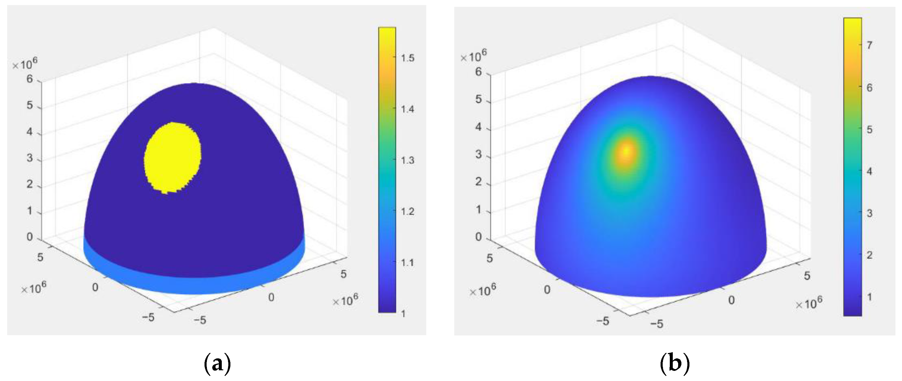
In calculating the sky diffuse irradiance in a narrow surface sky view, the traditional solution of the sky diffuse irradiance can be improved by ascending the sky lattice discretization precision and applying a more accurate sky diffuse radiation model. It is suggested to replace the traditional Perez model with the Igawa model for the radiation intensity distribution rendering.

(3)

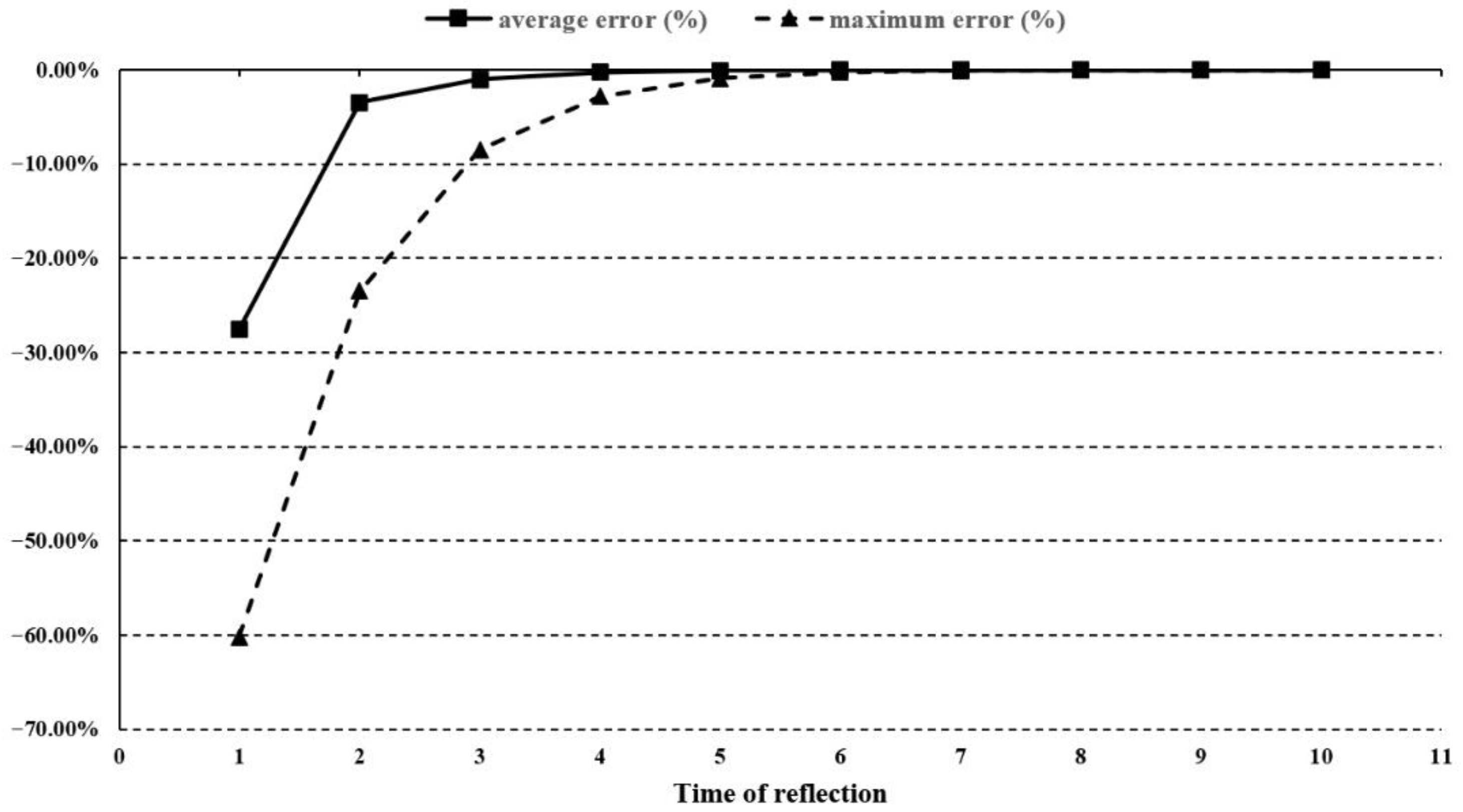
Compared with the infinite reflection algorithm, the existing mainstream one-time reflection algorithm has a significant error, especially on the surface where the radiation can reach only after multiple reflections. Such an error increases with the increase of the floor area ratio and the reflectivity of the building complex. It is recommended to use the infinite reflection algorithm, based on the net radiation analysis method in simulating the reflection irradiance of building facades. When the calculation resources are limited, the maximum error can be maintained within 5% by applying the four-time reflection algorithm.

Potential limitations of this work include the relatively limited measurements carried out by other scholars, which are related to the validity of the results by using the IFBS algorithms. As theoretically illustrated in this paper, the IFBS model will achieve a higher level of accuracy than traditional models, by applying more advanced models and algorithms. However, getting as many measurement studies as possible is necessary to verify the improvement in the accuracy of the IFBS model, compared with the traditional model. Unfortunately, few measurement studies have been carried out under the narrow sky view, and the corresponding methods and instruments are difficult to obtain. Therefore, future work on this paper will focus on the above problem.

References

1. Firth, S.K.; Lomas, K.J.; Wright, A. Investigating CO2 emission reductions in existing urban housing using a community domestic energy model. Proc. Build. Simul. 2009, 9, 2098–2105. [Google Scholar]
2. Heiple, S.; Sailor, D.J. Using building energy simulation and geospatial modeling techniques to determine high resolution building sector energy consumption profiles. Energy Build. 2008, 40, 1426–1436. [Google Scholar] [CrossRef] [Green Version]
3. Shimoda, Y.; Fujii, T.; Morikawa, T.; Mizuno, M. Residential end-use energy simulation at city scale. Build. Environ. 2004, 39, 959–967. [Google Scholar] [CrossRef]
4. Dascalaki, E.G.; Droutsa, K.G.; Balaras, C.A.; Kontoyiannidis, S. Building typologies as a tool for assessing the energy performance of residential buildings—A case study for the Hellenic building stock. Energy Build. 2011, 43, 3400–3409. [Google Scholar] [CrossRef]
5. Famuyibo, A.A.; Duffy, A.; Strachan, P. Developing archetypes for domestic dwellings—An Irish case study. Energy Build. 2012, 50, 150–157. [Google Scholar] [CrossRef] [Green Version]
6. Caputo, P.; Costa, G.; Ferrari, S. A supporting method for defining energy strategies in the building sector at urban scale. Energy Policy 2013, 55, 261–270. [Google Scholar] [CrossRef]
7. Aksoezen, M.; Daniel, M.; Hassler, U.; Kohler, N. Building age as an indicator for energy consumption. Energy Build. 2015, 87, 74–86. [Google Scholar] [CrossRef]
8. Krayenhoff, E.S.; Voogt, J.A. A microscale three-dimensional urban energy balance model for studying surface temperatures. Bound.-Layer Meteorol. 2007, 123, 433–461. [Google Scholar] [CrossRef]
9. Bruse, M.; Fleer, H. Simulating surface–plant–air interactions inside urban environments with a three dimensional numerical model. Environ. Modell. Softw. 1998, 13, 373–384. [Google Scholar] [CrossRef]
10. Hong, T.; Jiang, Y. A new multizone model for the simulation of building thermal performance. Build. Environ. 1997, 32, 123–128. [Google Scholar]
11. Nunez, M.; Oke, T.R. The energy balance of an urban canyon. J. Appl. Meteorol. 1977, 16, 11–19. [Google Scholar] [CrossRef]
12. Masson, V. A physically-based scheme for the urban energy budget in atmospheric models. Bound.-Layer Meteorol. 2000, 94, 357–397. [Google Scholar] [CrossRef]
13. Yang, X.; Li, Y. Development of a Three-Dimensional Urban Energy Model for Predicting and Understanding Surface Temperature Distribution. Bound.-Layer Meteorol. 2013, 149, 303–321. [Google Scholar] [CrossRef]
14. Quan, S.J.; Li, Q.; Augenbroe, G.; Brown, J.; Yang, P.P.-J. Urban data and building energy modeling: A GIS-based urban building energy modeling system using the urban-EPC engine. In Planning Support Systems and Smart Cities; Springer: Berlin, Germany, 2015; pp. 447–469. [Google Scholar]
15. Li, Z.; Xing, H.; Augenbroe, G. Criterion based selection of sky diffuse radiation models. Sustain. Cities Soc. 2019, 50, 101692. [Google Scholar] [CrossRef]
16. Liu, B.Y.H.; Jordan, R.C. The long-term average performance of flat-plate solar-energy collectors. Sol. Energy 1963, 7, 53–74. [Google Scholar] [CrossRef]
17. Perez, R.; Stewart, R.; Arbogast, C.; Seals, R.; Scott, J. An anisotropic hourly diffuse radiation model for sloping surfaces: Description, performance validation, site dependency evaluation. Sol. Energy 1986, 36, 481–497. [Google Scholar] [CrossRef]
18. Perez, R.; Seals, R.; Ineichen, P.; Stewart, R.; Menicucci, D. A new simplified version of the perez diffuse irradiance model for tilted surfaces. Sol. Energy 1987, 39, 221–231. [Google Scholar] [CrossRef] [Green Version]
19. Reinhart, C. Daysim, Advanced Daylight Simulation Software. 2013. Available online: http://daysim.ning.com (accessed on 27 June 2015).
20. Ward, G.; Shakespeare, R. Rendering with Radiance: The art and science of lighting visualization; Morgan Kaufmann: San Francisco, CA, USA, 1998. [Google Scholar]
21. Arnfield, A.J. Two decades of urban climate research: A review of turbulence, exchanges of energy and water, and the urban heat island. Int. J. Climatol. J. R. Meteorol. Soc. 2003, 23, 1–26. [Google Scholar] [CrossRef]
22. Terjung, W.H.; Louie, S.S.F. A Climatic Model of Urban Energy Budgets. Geogr. Anal. 1974, 6, 341–367. [Google Scholar] [CrossRef]
23. Siegel, R.; Howell, J.R. Thermal Radiation Heat Transfer; McGraw Hill: New York, NY, USA, 1972. [Google Scholar]
24. Wang, B.; Liu, G. Recalculation of common astronomical parameters in solar radiation observation. J. Sol. Energy 1991, 1, 27–32. [Google Scholar]
25. Yan, Q.; Zhao, Q. Heat Process in Buildings; Building Industry Press of China: Beijing, China, 1986. [Google Scholar]
26. Jensen, H.W. Realistic Image Synthesis Using Photon Mapping; Ak Peters: Natick, MA, USA, 2001; Volume 364. [Google Scholar]
27. Chen, C.W.; Hopkins, G.W. Ray tracing through funnel concentrator optics. Appl. Opt. 1978, 17, 1466–1467. [Google Scholar] [CrossRef]
28. Daly, J.C. Solar concentrator flux distributions using backward ray tracing. Appl. Opt. 1979, 18, 2696–2699. [Google Scholar] [CrossRef]
29. Leutz, R.; Annen, H.P. Reverse ray-tracing model for the performance evaluation of stationary solar concentrators. Sol. Energy 2007, 81, 761–767. [Google Scholar] [CrossRef]
30. Jaffey, A.H. Solid angle subtended by a circular aperture at point and spread sources: Formulas and some tables. Rev. Sci. Instrum. 1954, 25, 349–354. [Google Scholar] [CrossRef]
31. Tregenza, P.R.; Waters, I. Daylight coefficients. Light. Res. Technol. 1983, 15, 65–71. [Google Scholar] [CrossRef]
32. Ng, E.; Cheng, V.; Gadi, A.; Mu, J.; Lee, M.; Gadi, A. Defining standard skies for Hong Kong. Build. Environ. 2007, 42, 866–876. [Google Scholar] [CrossRef]
33. Li, D.H. A review of daylight illuminance determinations and energy implications. Appl. Energy 2010, 87, 2109–2118. [Google Scholar] [CrossRef]
34. Oke, T.R. Canyon geometry and the nocturnal urban heat island: Comparison of scale model and field observations. J. Climatol. 1981, 1, 237–254. [Google Scholar] [CrossRef]
35. van Esch, M.M.E.; Looman, R.H.J.; de Bruin-Hordijk, G.J. The effects of urban and building design parameters on solar access to the urban canyon and the potential for direct passive solar heating strategies. Energy Build. 2012, 47, 189–200. [Google Scholar] [CrossRef]
36. Davies, J.; Hay, J. Calculation of the Solar Radiation Incident on an Inclined Surface. In Proceedings of the First Canadian Solar Radiation Data Workshop, Toronto, ON, Canada, 17–19 April 1978; Hay, J.E., Won, T.K., Eds.; 1980; pp. 32–58. [Google Scholar]
37. Temps, R.C.; Coulson, K.L. Solar radiation incident upon slopes of different orientations. Sol. Energy 1977, 19, 179–184. [Google Scholar] [CrossRef]
Figure 1. Schematic diagram of the analysis of the radiation energy balance on the element surface.
Buildings 12 01914 g001
Figure 2. Light beam occlusion judgment, based on the backward ray tracing method.
Buildings 12 01914 g002
Figure 3. Definition of the solid angle in the spherical coordinate system.
Buildings 12 01914 g003
Figure 4. Fish eye photo in the building stocks environment.
Buildings 12 01914 g004
Figure 5. Influence of the sky lattice model on the expression of the sky diffuse radiation intensity. (a) Rendering of a real sky diffuse radiation intensity distribution. (b) Rendering, based on the Tregenza145 lattice model.
Buildings 12 01914 g005
Figure 6. Influence of the sky lattice model on the occlusion rendering. (a) Real sky occlusion rendering. (b) Tregenza145 model occlusion rendering.
Buildings 12 01914 g006
Figure 7. Schematic diagram of the sky lattice.
Buildings 12 01914 g007
Figure 8. Schematic diagram of the surface discretization.
Buildings 12 01914 g008
Figure 9. Distribution of the sky radiation intensity, based on the Tregenza145 sky lattice model. (a) Expression of the Perez model. (b) Expression of the Igawa model.
Buildings 12 01914 g009
Figure 10. Distribution of the sky radiation intensity, based on the sky lattice of the IFBS model algorithm. (a) Expression of the Perez model. (b) Expression of the Igawa model.
Buildings 12 01914 g010
Figure 11. Comparison of the calculation errors of the finite reflection radiation algorithms.
Buildings 12 01914 g011
Figure 12. Relative deviation of the reflection irradiance calculated by the finite time reflection algorithm for the building complexes. (a) one-time reflection algorithm. (b) two-time reflection algorithm.
Buildings 12 01914 g012