Shared PV Systems in Multi-Scaled Communities

Abstract

In past years, Sweden has been facing a rapid growth of photovoltaic cells, and the total PV installation capacity increased from 300 kW to 1090 MW (2006–2020). The increased number of PV users was a result of active support from the Swedish government with an aim of achieving multiple sustainable goals regarding renewable energy. This project evaluates the profitability of shared PV systems in communities of different sizes in Sweden. This study aimed to contribute to the literature by filling the research gap of presenting the financial benefits at different community scales. The electricity use profiles consisted of hourly measured electricity use that was derived from 1067 individual Swedish apartments. The profiles were then used to create multi-scaled communities with shared PV systems. The mid-market price model was implemented to simulate electricity trading among prosumers in the community using Visual Basic Applications (VBA) in MS Excel. Further, the electricity costs were used for Life Cycle Cost (LCC) assessment. To demonstrate the increase in profitability, the LCC results of households with shared PV systems were compared to households that own PV individually and households that do not own a PV system. The evaluation showed the financial benefits of shared PV systems in comparison with individually owned PV systems. This study also demonstrated the increase in profitability and the reduction in payback time for the average household if sharing a PV system as part of a larger community.

1. Introduction

The United Nations’ seventh sustainable development goal describes several targets regarding clean energy, including an increase in the renewable energy share in the global energy mix. Regarding solar power technology, the use of photovoltaic (PV) cells has been rapidly growing in Sweden since 2006. According to data collected by the National Survey of PV Power in Sweden (NSPS), it went from 300 kW of PV capacity installed in 2006 to nearly 1090 MW in 2020 [1]. This demonstrates how popular PV systems are becoming in the Swedish market. More homeowners are willing to invest in PV panels for a variety of reasons, including environmental concerns and profitability [2].

In Sweden, retail electricity costs are still higher than the costs of self-produced electricity. The use of self-produced electricity reduces the amount of purchased electricity, hence increasing the user’s profitability [3]. Along with that, the usage of self-produced electricity reduces the pressure on local electricity companies, who are often affected by the electric grid’s supply and demand imbalance [4]. Despite the net-metering type, buying prices significantly increase during high demand and the price for selling surplus electricity declines during low demand. That, in turn, negatively affects PV owners [5].

Other European countries addressed the grid’s imbalance issue with a concept known as Smart Grid [6]. Basically, users started to apply electricity management technologies consisting of metering devices and sensors to circulate electricity use information between utility company and the users [7]. Within the Smart Grid context, the concepts of microgrids and energy communities were created. In simple terms, electricity consumers locally producing renewable energy, who were usually referred to as “prosumers”, form a community to share PV electricity production [8]. By aggregating the prosumers electricity demand, it allowed them as a community to use more self-produced electricity and rely less on the grid’s electricity [9].

The temporal difference of the combined electricity demands reduces the number of hours when PV electricity is not being used [9,10]. Given that, recent research on PV system sharing has been developing models to prove its applicability in real cases. These models treat an energy community as a trading zone. Basically, prosumers trade their electricity surplus with other prosumers in electricity shortage. To do so, these models count with an entity, known as an aggregator, or Energy Sharing Provider (ESP) [11]. This entity (e.g., third party company) intermediates the electricity trading between prosumers themselves and the utility grid. By being impartial, the aggregators can balance electricity supply and demand within a prosumers’ community [12].

State-of-the-Art

A previous study investigated the possible benefits of shared PV systems [13]. The study’s case consisted of real measured electricity load profiles of few different settlements (single-family houses, multi-apartment buildings, historical buildings, and commercial facilities). The settlements not only had different electricity-providing sources but also roof top spaces and constraints for PV panels installation. The study determined the efficiency of an electricity sharing community for each type of settlement. Single-family houses profited more from the synergy of different load profiles, and multi-apartment buildings presented the highest cost reduction within the settlement types.

Research conducted in Portugal [14], where PV sharing is regulated, emphasizes the benefits of PV sharing, especially when focusing on increased self-use. It also explores different models of energy communities to share PV electricity. The proposed model in the paper consisted of an apartment building sharing PV electricity with the assistance of an energy aggregator to manage the distribution of electricity. The analysis considered the use of batteries to store the part of the electricity not being utilized.

Moreover, more research [9] provided an analysis about load aggregation using electricity use data of 18 households and three small shops in Portugal. It revealed an improvement in self-use between 50% and 80% by just aggregating 10 households’ loads and using a 1 kWh/kWp battery. Additionally, a 90% self-use increase was reported when considering the small shops in the load aggregation. The study depicts the increase of self-use and profitability in relation to individually owned PV systems.

Another previous study [10] compared eight countries (Austria, Germany, Netherlands, Belgium, France, Italy, Spain, and Portugal) in terms of cost reduction when forming an energy community where PV electricity is sharable. In the study, two scenarios were analyzed. The first one included a carbon-based society, where energy for producing heat and operating transportation were provided by fossil-fuels. The second one represented a full-electric scenario that considered the use of heat pumps to provide heat and electric vehicles as the main transportation. However, the last scenario presented higher electricity use. Using simulated load profiles, the results presented energy cost reduction for all countries when implementing PV systems and even higher cost reduction when sharing PV systems. With high electricity prices in countries like Germany, Belgium, and Netherlands, PV system sharing becomes even more profitable through the increased self-use of PV electricity.

Yet another study [15] proposed three different models for peer-to-peer (P2P) electricity trading in a microgrid using PV electricity. The models, so called bill-sharing, mid-market rate, and action-based pricing, were composed of different pricing rules for trading electricity. The study shows that it was possible to reduce electricity costs up to 30% using any of the proposed P2P electricity trading models, and the main driver for such reduction was the diversity of load schedules. Furthermore, the study concluded that the use of P2P electricity trading can be used for residential microgrids on a large scale.

Within the same topic, two other studies [12,16] proposed models of PV sharing integrated with demand-side management, a Smart Grid approach to managing electricity demand. The microgrids worked as electricity trading zones with internal electricity prices. These internal prices could change according to the electricity supply-and-demand ratio of the microgrid. Both models presented positive revenue when compared with direct electricity trading between PV prosumers and utility grid.

Nevertheless, there is scant research about the increasing financial benefits of different communities’ scales. Therefore, the main goal of this research is to demonstrate the financial profitability of shared PV systems in different community sizes. The paper not only demonstrates how much more profitable it is to share PV systems’ electricity when compared to individually owned PV systems but also how much the profitability of a participating household grows if increasing the size of the community.

One of the limitations of this study is the focus on Swedish residential apartment buildings, not extending the research to other types of dwellings. The focus on Swedish apartments aimed to increase the results’ accuracy since the electricity data comes from real measurements in apartments located in Karlstad, Sweden. Additionally, only PV systems without a battery/storage system were considered in this study. This article is based on an original study that used a large database of measured electricity use profiles. The large number of electricity profiles allowed a very precise basis for calculations and therefore brings scientific value to the literature on shared PV systems. The findings, methods, and approaches provided in this study could be used to evaluate the potential profitability for various combined electricity use profiles at an international level.

2. Materials and Method

The following methodology section presents the detailed step-by-step process needed to calculate profitability of shared PV systems (Figure 1). Using Visual Basic Applications (VBA) in MS Excel, electricity use profiles were combined randomly using a database with pre-measured electricity use from 1067 households. A more detailed description of the profiles is given in Section 2.1. The household electricity profiles in each combination were further matched with PV supply that was simulated using System Advisor Model (SAM) software [17]. Additionally, based on the electricity balance calculations (Section 2.5), an electricity trading scheme was applied to simulate the exchange of electricity among prosumers (Section 2.6). Further on, LCC was calculated in three cases: households sharing a PV system within communities of different sizes, owning a PV system without sharing it, and without a PV system. The LCCs were further compared to determine the profitability for each household in different situations (sharing, not sharing, and without a PV system).

2.1. Database of Household Electricity Profiles

The data consisted of household electricity use profiles that was obtained [18] and analyzed as a part of previous research [19]. The electricity measurements were taken in 2012 from 1509 apartments of varied sizes in several buildings in a Swedish city called Karlstad with approximately 95,000 inhabitants, located at latitude 59°. However, the gathered data needed to be filtered and verified. According to previous research [19], several errors and strange patterns were detected, such as profiles with more than 3% of missing data or other anomalies like very high averages or inexplicable spikes. Finally, only 1067 profiles that passed the 3% missing data limit and visual inspection were verified and therefore included in the initial dataset of this research.

According to the bureau of Swedish statistics (SCB) [20], the population of the municipality is demographically representative of Sweden. Approximately 75% of the apartments in mixed residential blocks contained two or three rooms and a kitchen; the rest of the 25% were five-room apartments with a kitchen and just a few six-room apartments. The household electricity usage included electricity for light, electrical appliances, and equipment, along with electric towel racks in the bathrooms.

2.2. PV Electricity Supply

In this study, SAM software [17] was used to simulate the hourly supply of PV electricity for a whole year. The weather data was chosen to correspond with the location of the households that had their electricity use measured, i.e., Karlstad, Sweden. The file containing the weather data is in the International Weather for Energy Calculations (IWEC) format. Files in this format consist of collected weather data from up to 18 years, including solar radiation data that is estimated on an hourly basis. It represents the weather of a typical year in the selected location [21]. According to the weather data file, the annual average temperature in Karlstad, Sweden, is 5.9 °C, and the annual radiation on the horizontal surface is 1000 kWh/m².

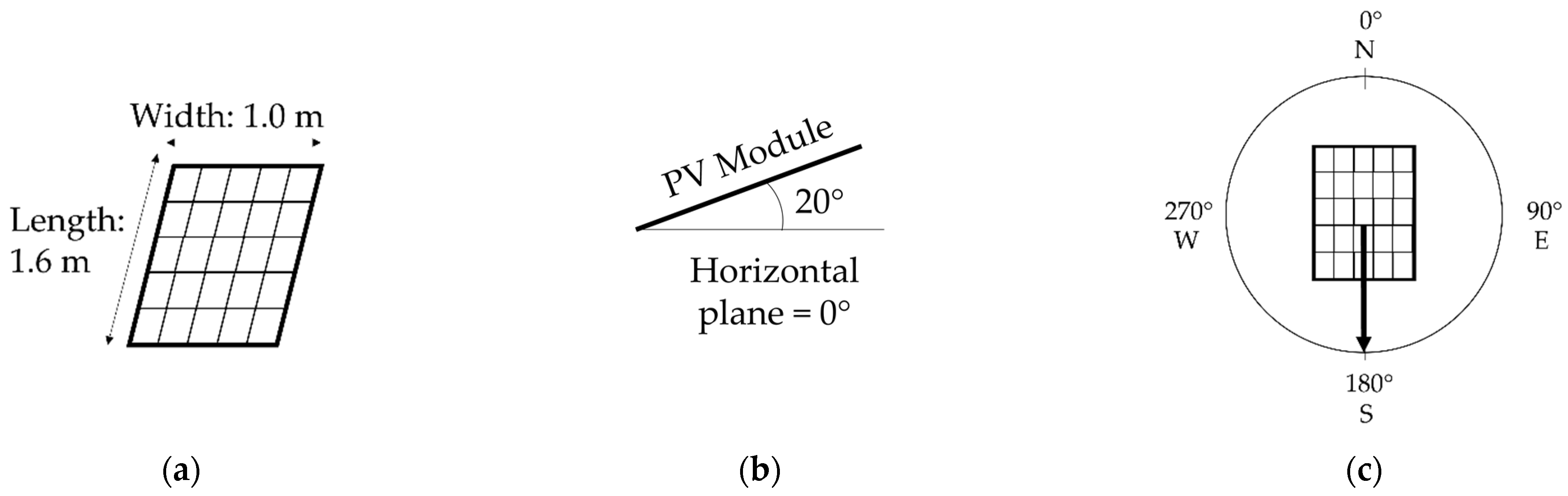
Since the main objective of this research was investigating the potential of sharing PV systems, it was necessary to assume that each household within a community had the same PV system size and configuration (modules’ tilt and orientation). Using SAM software, the supply of several PV system sizes was simulated and then manually compared to the demand of every single household electricity profile in the database. The electricity savings provided by the supply of each system was compared to their cost. The aim of this comparison was to identify the range of PV system sizes that would present the highest financial benefit above others. Based on that, four PV sizes (0.25 kWp, 0.5 kWp, 0.75 kWp, and 1 kWp) were further analyzed and presented in this paper. The PV systems consisted of modules with 20% efficiency and dimensions of 1.6 m × 1.0 m (Figure 2a). The modules were tilted at an angle of 20° (Figure 2b) and with an azimuth of 180°, which corresponds to the south orientation (Figure 2c). This configuration can be found as a recommendation for flat roof buildings by Swedish solar panel retailers [22,23]. The tilt of the module is lower than the optimal tilt for Swedish locations (around 40°) to maximize the number of solar panels in the roof space without the panels shading each other.

Furthermore, shading from other objects on the modules was not considered in order to simplify the study’s analysis. By considering shading, the PV electricity production would be reduced in all cases. Losses due to dust or other soiling on the modules were considered to be 5%. Soiling or dust loss values can vary according to the installation location. Previous research [24] stated the variation of those losses, 4.4% in Spain and from 1.1% to 6.9% in Italy.

2.3. Statistical Approach for Sampling

Probability sampling was used to determine the number of samples needed for the analysis. Every combination in the population has a non-zero chance of being selected, so the sample is completely aleatory [25]. For each combination size, the term “population” refers to all possible combinations that can be made with the 1067 household electricity profiles, and the term “sample” refers to a single combination.

According to earlier research [26], it is more reasonable to employ sampling than census, which involves analyzing the entire population and is more suitable for small groups. However, this brings the issue of choosing a sample size large enough to represent the whole population’s statistical characteristics. The Yamane equation, which is specifically designed for determining the sample size for large populations [25], is defined as

$$n=\frac{N}{1+N · e^2}$$

(1)

in which a desired margin of error is used to decide the number of samples, considering that the population’s standard deviation is unknown.

In the equation, the number of samples is symbolized by “n”, the population by “N”, and “e” represents the desired margin of error. As it shows in Figure 3, for larger populations, the equation result is mainly influenced by the chosen margin of error, and it barely changes from 400 samples. It is important to note that two electricity profiles are the bare minimum that can be combined. Additionally, repeated selection is allowed, i.e., selecting a repeated electricity profile in the same combination, resulting in more than 8000 possible combinations. In this study, a margin of error of 0.05 was considered to determine the number of samples. Hence, 400 samples were chosen to suit the study’s time and computational limitations.

2.4. Randomized Combinations

The random selection method was used to create household combinations, using VBA-coding application in MS Excel. The combination sizes were set to be for 2, 5, 10, 20, and 50 households.

All household profiles from the initial database were included in a randomization process. By using a random selection function, the necessary number of participants was grouped into one combination by randomly selecting profiles from the available database of 1067 electricity use profiles (Figure 4). The total population of profiles was considered for selection in every independent run of the randomization process, so previously selected profiles were free to be selected for multiple runs. The randomization was finalized by creating a database with all created combinations.

2.5. Electricity Balance

The electricity balance concept represents the correlation of household’s electricity demand with PV electricity supply. Figure 5 shows an example of hourly household electricity together with PV electricity supplied during a 24 h period. From the chart, two curves can be observed: the household electricity use and PV electricity supply, in which the hourly difference between these curves is called the electricity balance (B).

In each hour (t), the electricity balance (B) was calculated for an individual household, referred to as n, using Equation (2). The supplied PV electricity was considered as S(t) and the used household electricity as U(t). When the equation’s result is negative (−), it depicts electricity that needs to be bought (E_b) (Equation (3)). When the result is positive (+), it depicts a surplus of electricity that could be sold (E_s) (Equation (4)). Moreover, if the result is equal to zero, it means that the PV electricity supply matched the electricity use.

$$B_n\left(t\right)=S_n\left(t\right)-U_n\left(t\right)$$

(2)

$$E_{b n}\left(t\right)=\{\begin{array}{c}-B_n\left(t\right), B_n<0\\ 0, B_n\ge 0\end{array}$$

(3)

$$E_{s n}\left(t\right)=\{\begin{array}{c} 0, B_n\le 0\\ B_n\left(t\right), B_n>0\end{array}$$

(4)

Every single household from the 1067 was coupled with a PV system. This was done for the PV systems of size 0.25 kWp, 0.5 kWp, 0.75 kWp, and 1 kWp. Finally, the electricity balance was calculated for all 8760 hours of the year for each household with the previously mentioned PV systems.

2.6. Electricity Trading

A price model proposed by previous research [15], the so-called mid-market rate, was used in the calculation of the electricity cost for a household trading electricity within a community. The electricity trading method and equations developed in this paper were based on previous research [15]. Considering the electricity user’s perspective, three prices were considered in the model: the hourly price to buy electricity from the electricity grid (Pr_bg), to sell electricity to the electricity grid (Pr_sg), and the hourly price of buying or selling electricity from and to other households (Pr_c). In the model, Pr_c is assumed as the average of Pr_bg and Pr_sg. Figure 6 shows the price scheme with an example of a three-household community trading electricity.

In a community, each household uses their PV system supply to satisfy their whole electricity demand or at least part of it. After that, some of the households can still have electricity available to sell, while others still need to purchase electricity. Considering all the households, the amount of available electricity and electricity that needs to be purchased are respectively called the community’s electricity offer (El_offer) and demand (El_demand). Equations (5) and (6) shows the calculation of El_offer and El_demand, respectively.

$$E{l}_{offer}\left(t\right)={{\displaystyle \sum }}_{n=1}^N{E}_{s n}\left(t\right)$$

(5)

$$E{l}_{demand}\left(t\right)={{\displaystyle \sum }}_{n=1}^N{E}_{\mathrm{b} n}\left(t\right)$$

(6)

In different hours, offer and demand for electricity within a community can vary. When electricity offer matches electricity demand (El_offer = El_demand), all of the electricity can be traded among households at the trading price (Pr_c). Households do not need to sell or buy electricity to or from the grid. In that case, an individual household’s electricity cost (C) is obtained by

$$C_n \left(t\right)=\{\begin{array}{c}{E}_{\mathrm{b} n}\left(t\right) · P{r}_c \left(t\right), B_n\left(t\right)<0\\ – E_{s n}\left(t\right) · P{r}_c \left(t\right), B_n\left(t\right)>0 \end{array} if E{l}_{offer}=E{l}_{demand}$$

(7)

At a certain hour, the electricity offer can be higher than electricity demand (El_offer > El_demand). So first, the community’s electricity demand is fully satisfied by trading part of the electricity surplus among households. Thus, the amount of electricity surplus sold at trading price (Pr_c) is equal to the amount of electricity demand (El_demand). The remaining amount of electricity surplus is then sold back to the grid at electricity grid’s price (Pr_sg). Therefore, the community’s profit from sold electricity (P_s) is defined as

$$P_s\left(t\right)=E{l}_{demand}\left(t\right) · P{r}_c\left(t\right)+\left(E{l}_{offer}\left(t\right)-E{l}_{demand}\left(t\right)\right) · P{r}_{sg}\left(t\right)$$

(8)

The profit is shared among the households that sell electricity surplus. The share of each household is determined by the ratio of their individual electricity surplus and the community’s electricity offer. Hence, an individual household’s electricity cost is given by

$$C_n \left(t\right)=\{\begin{array}{c}{E}_{\mathrm{b} n}\left(t\right) · P{r}_c\left(t\right), B_n\left(t\right)<0\\ \frac{– E_{s n}\left(t\right)}{E{l}_{offer}\left(t\right)} · P_s\left(t\right), B_n\left(t\right)>0 \end{array} if E{l}_{offer}>E{l}_{demand}$$

(9)

On the other hand, a community’s electricity demand can be higher than its electricity offer (El_offer < El_demand). In that case, all of the electricity surplus is traded among households to satisfy part of the electricity demand. Therefore, the amount of electricity being purchased at the trading price (Pr_c) is equal to the amount of offered electricity (El_offer). The lacking electricity is then bought from the grid at electricity grid’s price (Pr_bg). Therefore, the community’s electricity cost (P_b) is defined as

$$P_b\left(t\right)=E{l}_{offer}\left(t\right) · P{r}_c\left(t\right)+\left(E{l}_{demand}\left(t\right)-E{l}_{offer}\left(t\right)\right) · P{r}_{bg}\left(t\right)$$

(10)

This cost is also shared, but this time among the households that still need to buy electricity after using their own produced electricity. The share of each household is determined by the ratio of their individual electricity need and the community’s electricity demand. Thus, an individual household’s electricity cost is determined by

$$C_n \left(t\right)=\{\begin{array}{c}\frac{E_{\mathrm{b} n}\left(t\right)}{E{l}_{demand}\left(t\right)} · P_b\left(t\right), B_n\left(t\right)<0\\ – E_{s n}\left(t\right) · P{r}_c \left(t\right), B_n\left(t\right)>0 \end{array} if E{l}_{offer}<E{l}_{demand}$$

(11)

2.7. LCC Calculation

For a household, referred as n, the LCC was calculated considering the PV system investment cost (C_inv), the system’s maintenance (C_main), and the annually purchased electricity (C_el.purchased). The annual purchased electricity cost was determined by just summing the electricity costs in all 8760 h, as shown in Equation (12). Hence, by considering a certain number of years (Y) and using an interest rate (i), an electricity price growth rate (g) and a maintenance cost growth rate (m), the net present value (NPV) for the cashflows C_main and C_el.purchased can be calculated as shown in Equations (13) and (14) [27]. Finally, the LCC was the sum of the investment cost and the NPV for maintenance and purchased electricity cost as it is shown in Equation (15).

$$C_{el. purchased n}={\displaystyle \sum }_{t=0}^{8760}{C}_n\left(t\right)$$

(12)

$$NP{V}_{main n}=C_{main n} ·\left(1+m\right)·\frac{\left(1-{\left(1+m\right)}^Y · {\left(1+i\right)}^Y\right)}{i-m}$$

(13)

$$NP{V}_{el.purchased n}=C_{el. purchased n} ·\left(1+g\right)·\frac{\left(1-{\left(1+g\right)}^Y · {\left(1+i\right)}^Y\right)}{i-g}$$

(14)

$$LC{C}_n=C_{inv n}+NP{V}_{main n}+NP{V}_{el. purchased n}$$

(15)

The financial assessment of the cases was carried out to monetize expenses and income for households that participated in combinations. Life cycle costs calculations were performed for a period of 40 years. The scope of analysis included initial investment, maintenance, and electricity costs.

The initial and maintenance costs were based on the market situation, according to the NSPS [1]. Both types of costs were calculated individually for each household, according to the size of their PV system. It also means that, in case of shared PV systems, the initial and maintenance costs were not shared between participants.

Below one can find the list with the cost parameters considered in the LCC calculation:

• 16090 SEK/kWp for initial costs (PV system cost and installation, inverter and meter);
• 2040 SEK/kWp for the inverter change each 10 years;
• 3170 SEK/kWp for the PV modules change each 25 years;
• 2% growth rate applied to the costs of the PV modules and inverter change;
• 1.9% interest rate.

The maintenance cost growth rate was based on the consumer price index (CPI) from previous years [28] The interest rate was calculated based on the data from previous years (2016–2019), according to SCB [20].

Electricity costs included running costs for purchased and sold electricity and were based on hourly spot prices from 2019, since it was the last year before the Corona pandemic affected the energy market. The spot price was given hourly according to Nord Pool [29]. In addition, all trading and network fees were calculated and added based on the data from the biggest electricity provider of the region where the electricity profiles are located [30,31]. It is worthwhile to note that only the variable type of electricity contract was considered, as it allowed for more transparent data from electricity providers. To set assumptions for growth rates, the average of electricity trading and network prices in the region was calculated based on archive data from past years (2016–2020) [32].

Below is a list with the considered inputs of hourly electricity prices and growth rate according to the price scenario of 2019:

• Vattenfall was identified as the biggest electricity provider in the region;
• Network fixed fee of 0.0205 SEK/hour plus 0.31 SEK/kWh of variable fee;
• Electricity price growth rate of 2%;
• All prices include a VAT of 25%.

In the current tax system of Sweden, the subsidies for PV ownership are an important tool to create awareness of the potential and value of PV systems [1]. However, it is impossible to make predictions regarding tax reduction changes over the years. Tax reduction rules could change rapidly, according to governmental goals [1]. Therefore, the main LCC calculations initially excluded tax reduction, but the impact of it was studied in the sensitivity analysis. The option for selling electricity certificates was not taken into account in this study.

2.8. Sensitivity Analysis for LCC

The sensitivity analysis followed the Morris method [33], in which one parameter is changed at a time in each simulation run. Two parameters in the LCC calculations were considered for the sensitivity analysis: the electricity price growth rate and the implementation of a tax reduction benefit. The first step of the sensitivity analysis consisted of calculating the results for a slightly increased electricity price growth of 3% [20], assuming a scenario where electricity becomes more expensive. The results were then compared to the results with an electricity price growth of 2%.

The second step was to consider a tax reduction benefit applied to the electricity surplus that is sold from individual households to the grid. According to the latest data, PV micro producers in Sweden that produce a maximum of 43.5 kW while selling less electricity than they consume from the main grid, are accounted for a tax reduction of 0.6 SEK/kWh. The calculated amount is added to their income from selling surplus electricity to the main grid [34]. Results for households owning an individual PV system were then compared in two situations: with and without the tax reduction benefit. Those results were also compared to the results of households sharing their PV system without the tax reduction benefit.

2.9. Profitability

The profitability is defined as making a profit when the time to recover investment was shorter than the project’s lifespan. The calculation method was applied to compare different scenarios and draw the difference between single households that were a part of a shared PV community, own PV individually without sharing, or do not use PV at all. It was implemented through a formula that extracts the difference between LCC costs and therefore validates the potential savings of choosing one scenario over another, as was presented in the Equation (16).

$$Profitability=LC{C}_{withPV}-LC{C}_{noPV}$$

(16)

To establish common ground, LCC for a case with no PV system ($LC{C}_{noPV}$) was chosen. It was further compared with the LCC ($LC{C}_{\begin{array}{c}withPV\end{array}})$ of a household owning a shared PV system and owning a PV system individually. As a result, using the same formula, two types of profitability were extracted: for cases wherein households share their PV with others and wherein they own PV systems individually.

3. Results

This section presents the results as the average profitability and payback of all households participating in 400 samples. The results first show the electricity balance of an average household in Karlstad (Section 3.1). The households’ profitability and payback period are also presented (Section 3.2). It is followed by the sensitivity analysis, which shows the results of a single-household profit including the tax reduction benefit (Section 3.3). Those results are compared with the profitability results from the previous sections.

3.1. Electricity Balance of an Average Household

Figure 7 shows the PV supply of a 1 kWp system with a 180° azimuth and a 20° tilt and the electricity use of an average household in Karlstad based on profiles from the initial database. A mismatch can be observed between the average electricity use profile and PV supply for Karlstad. This mismatch can be seen during the winter months, when the electricity demand is high, but the solar supply is low due to shorter days. It depicts well the typical situation in Sweden, where, due to the geographical location, the self-use can be reduced by the electricity imbalance.

3.2. Profitability and Payback

In this section, profitability results were analyzed over a period of 40 years, and it does not consider the tax reduction benefit. Figure 8 shows the average household profitability in combinations of 1, 2, 5, 10, and 50 households, with a 0.25 kWp system per household. The results were displayed for scenarios of electricity price growth of 2% and 3%.

It was observed that a household sharing a PV system presented higher profitability when compared to a household with an individual PV system. For example, with an electricity price growth of 2%, a household in a two-household combination presented a profit of 1610 SEK. It was an increase of 677 SEK when compared to the profit of 933 SEK for a household with an individual system. The average household profitability kept increasing as more households started to share PV systems. However, the greater the number of households included in the combination, the smaller the increase in profitability. It was also observed that the average household profitability increased in all combinations when the electricity price growth changed from 2% to 3%.

Further, Figure 9a,b shows the average household profitability for different PV systems (0.25 kWp, 0.5 kWp, 0.75 kWp, and 1 kWp) in the same combination sizes. Figure 9a shows the results for an electricity price growth of 2%, wherein the 0.25 kWp and 0.5 kWp systems remained profitable in all combinations. The 0.75 kWp system was only not profitable for one household with an individual system, and the 1 kWp was not profitable in any combination. Importantly, in combinations with more than two households, the 0.5 kWp system became more profitable than the 0.25 kWp system. Moreover, in Figure 9b, when electricity price growth is 3%, all four PV systems were profitable in all combinations, while the 0.75 kWp system was the most profitable.

Figure 10a shows the payback results for electricity price growth of 2%. It was noticed that the system’s payback can be reduced by up to 10 years when a household is sharing a PV system in a combination of five or more households. In Figure 10b, a reduction was also seen for the electricity price growth scenario of 3%, wherein the system’s payback can be reduced by up to 4 years. Moreover, for all four PV systems, the payback curves started to flatten after five-household combinations, presenting the same payback period in combinations of 10, 20, and 50 households.

In Figure 11a,b, average household profitability was analysed over the years to explain the difference in payback reduction between different scenarios of electricity price growth. In the analysis, the payback is represented by the year when the PV system becomes profitable for the first time. Recurrent costs such as the change of the inverter in the 30th year (Figure 11a,b) and the change of the module in the 25th year (Figure 11b) cause financial losses. Given that, more time is needed for a PV system to become profitable. It was observed for an individual PV system (1H) with an electricity price growth of 2% (Figure 11a) that profitability drops in the 30th year when the inverter is exchanged. After that year, profit is again achieved, making the system reach its payback in the 33rd year. The same case with an electricity price growth of 3% (Figure 11b) reaches its payback after 23 years, which is before the 25th year when PV modules are exchanged. As a consequence, the difference in payback time between an individual system and a shared system is smaller when considering an electricity price growth of 3%.

3.3. Sensitivity Analysis: Tax Reduction

Furthermore, the tax reduction benefit was implemented for the cases of households owning an individual PV system. Figure 12 shows the average profitability, wherein one household was compared in two situations: with tax reduction and without tax reduction. When considering the tax reduction benefit, one household presents higher profitability with any system size when compared to other cases without the tax reduction benefit. The only exception was for a system of 0.25 kWp, wherein it was more profitable when shared with other households.

4. Discussion

The results of this study demonstrate that shared PV systems were more profitable than individually owned PV systems. The profitability determined in this study was for a specific case: apartment buildings in Sweden. Results comparison with other studies can be complex and inaccurate due to the unique combination of parameters (e.g., electricity use profiles, location, electricity prices, system cost, etc.). The profitability magnitude depends on several factors, especially electricity prices. For example, considering higher electricity prices can substantially increase the profitability shown in this research.

The profitability of shared PV systems was achieved through electricity trading between households in residential communities. As previous research has demonstrated [11], prosumers can have more financial benefits trading electricity among themselves than trading with the electricity grid. It is also seen that households, with individual PV systems, can increase their PV system size when sharing it with other households to maximize their profit. The reason is the increase of the system’s electricity self-use when sharing it. However, when sharing PV with a large number of households, the difference in profitability is minimal; hence, the profit does not overcome the investment costs to own a bigger PV system. Furthermore, future research can investigate the average household profitability by using another pricing model or trading approach.

The implementation of an electricity trading scheme could impact the electricity usage in the apartments. The residents’ awareness of such a solution could affect their everyday habits, possibly increasing or decreasing their electricity use. Previous research has identified homeowners who use PV systems as a justification for the changes in their electricity use behaviour [35].

Electricity trading is enhanced by combining households with different electricity use behaviour. Combinations with a larger number of households have more electricity being traded than smaller combinations. However, as the combination size increases, the number of households with similar electricity use behaviour increases as well. Hence, a small difference in the average profitability between the larger combination sizes (10, 20, and 50 households) was observed.

The payback analysis showed that a household can reduce the PV system’s payback time by sharing PV electricity with other households. This aligns with earlier research [9] that demonstrated a reduction in payback time when comparing the sharing of PV systems with individually owning one. Reducing the PV system’s payback is beneficial since long payback periods are one of the main barriers that prevent homeowners from actively investing in PV systems [2].

The study’s method considered apartments where owners were allowed to install their own solar cells on the building’s roof and to share electricity production. The method can also be applied to single-family houses; however, there could be differences in terms of electricity use when comparing apartments to houses. If single-family households were to be considered, the accuracy of the results would be reduced. Moreover, future research can be focused on studying the combinations of profiles with different load variations, such as apartments, single-family houses, schools, and offices. This will provide larger variations and thus potentially increase the benefits of sharing.

Furthermore, the system’s installation could be potentially simplified with shared PV systems, for which not all apartments would need individual inverters or mounted structures on the roofs. This would make installation planning simpler and would reduce PV system costs. Moreover, other variables such as modules’ tilt, orientation, location (e.g., roof or landscape), and efficiency did not vary, to isolate the effect of different electricity profile combinations on the results. Future research could study the impact on profitability from changing the values of those variables.

The study did not investigate the willingness of PV owners to share their systems, nor how a community would be constructed. The research findings focused only on the financial outcomes of shared PV systems.

Finally, future climate impact was not considered in this study. According to the predictions of the Swedish Meteorological and Hydrological Institute (SMHI), the maximum temperature in Sweden will increase in all emission scenarios by 2040 [36]. Warmer temperatures could decrease the modules’ efficiency and result in lower electricity production. Consequently, it would reduce the profitability values for PV systems in all cases (individually owned and shared). Future research could explore the impact of future climate in the profitability of shared PV systems.

5. Conclusions

The research was focused on analysing profitability while looking at multi-scaled communities with shared PV systems. The goal was to demonstrate how profitable it was for an individual household to share a PV system in different community sizes and to compare it to when they used a system on their own.

Overall, the study’s findings demonstrated that:

• The individual profitability of a household was greater when PV systems were shared within a group of households than when the PV system was owned individually.
• The profitability of households was higher when they share electricity in larger communities. The study confirmed that, by sharing electricity with more households, the most profitable PV system’s size increases. However, it mostly affected smaller communities where the difference in profit was larger.
• Profitability increase was a result from electricity trading between households, where a price model was implemented. This enabled electricity trading to be more financially advantageous than exchanging electricity with the grid.
• The impact of the tax reduction benefit was analysed, and the results showed significant financial benefits. Currently, subsidies implemented by the government in Sweden are strong tools to motivate homeowners making decisions towards solar energy sources [37]. However, subsidies are directly dependent on governmental goals, so there is no guarantee that these would be in place during the following years [37]. Regardless of the tax reduction benefit, the results demonstrated that PV sharing is beneficial on its own.