Deep Forest-Based DQN for Cooling Water System Energy Saving Control in HVAC

Abstract

Currently, reinforcement learning (RL) has shown great potential in energy saving in HVAC systems. However, in most cases, RL takes a relatively long period to explore the environment before obtaining an excellent control policy, which may lead to an increase in cost. To reduce the unnecessary waste caused by RL methods in exploration, we extended the deep forest-based deep Q-network (DF-DQN) from the prediction problem to the control problem, optimizing the running frequency of the cooling water pump and cooling tower in the cooling water system. In DF-DQN, it uses the historical data or expert experience as a priori knowledge to train a deep forest (DF) classifier, and then combines the output of DQN to attain the control frequency, where DF can map the original action space of DQN to a smaller one, so DF-DQN converges faster and has a better energy-saving effect than DQN in the early stage. In order to verify the performance of DF-DQN, we constructed a cooling water system model based on historical data. The experimental results show that DF-DQN can realize energy savings from the first year, while DQN realized savings from the third year. DF-DQN’s energy-saving effect is much better than DQN in the early stage, and it also has a good performance in the latter stage. In 20 years, DF-DQN can improve the energy-saving effect by 11.035% on average every year, DQN can improve by 7.972%, and the model-based control method can improve by 13.755%. Compared with traditional RL methods, DF-DQN can avoid unnecessary waste caused by exploration in the early stage and has a good performance in general, which indicates that DF-DQN is more suitable for engineering practice.

1. Introduction

In order to achieve the goal of carbon neutrality, countries around the world are committed to energy saving and emission reduction. Building energy consumption accounts for a large part of energy consumption around the world [1], and heating, ventilation, and air-conditioning (HVAC) systems occupy a major part, reaching more than half of energy consumption. The cooling water system is an essential subsystem of the HVAC system, which mainly consists of cooling water pumps, cooling towers, and chiller condensers [2]. The operation of the cooling water system has an important influence on the entire HVAC system, and optimal control of the cooling water system can effectively reduce energy consumption of the HVAC system. Thus, the optimal control of the cooling water system is crucial.

In HVAC systems, optimal control policies are often used to reduce operation costs and to ensure the thermal comfort of occupants [3,4]. Optimal control policies can be classified into traditional control policies and advanced control policies in intelligent buildings, where the former one contains sequencing control (rule-based control) and process control, and the latter one includes soft-computing control policies, hard-computing control policies, and hybrid control policies [5]. Many optimal control methods have been tried for cooling water system control, such as proportional-integral (PI) controllers, proportional integral derivative (PID) controllers, and model predictive control (MPC) controllers. These methods heavily rely on the system model, various sensors, and controllers in the system, so the disadvantages of these methods are also obvious. Model-based methods often require a perfect model of the system, while system modeling is usually difficult in real applications even if we can attain enough data from different sensors. According to Zhu et al., the uncertainties of the model have a serious impact on the control performance [6]. In the actual system operation, the aging of the equipment or the renewal of some equipment may lead to inconsistency between the system model and the actual system [7]. Even if the initially established model is accurate enough, continuous changes in the actual system over time lead to an unavoidable decrease in the performance of the control method.

To avoid the impact of the imperfect system model on control policies, data-driving methods in artificial intelligence have received too much attention in HVAC control problems recently. Reinforcement learning (RL) is a kind of classical data-driven and model-free method in artificial intelligence. In recent years, RL has attracted increasing attention for building energy efficiency control problems [8,9], because it can provide a simple framework by learning from interaction with the environment directly. In these studies, RL methods can provide a model-free framework for achieving energy saving, but they often fail to achieve a good control effect in the early stage, or can be even worse than some baseline control policies, which are mainly caused by the agent’s exploration of the environment. Moreover, in the exploration process by the trial-and-error mechanism, they may also cause a certain degree of damage to the equipment, which may directly lead to an increase in cost. These two problems severely limit the practical use of RL in the field of HVAC optimization applications. Therefore, in order to maintain RL control effectiveness and achieve the maximum possible energy savings, it is necessary to reduce the time of this process in some way so that the RL control policy converges more quickly to reduce unnecessary costs.

In this paper, we tried to use DF-DQN to tackle this problem. Due to the introduction of DF, we mapped the original action space to a smaller one, and then combined the label of DF to attain the final control action, which directly reduced the output action of DQN. Moreover, the label of DF had the guidance of a priori knowledge, which not only ensured a good control effect, but also can realize energy saving in the early stage. The main contributions of this paper are as follows:

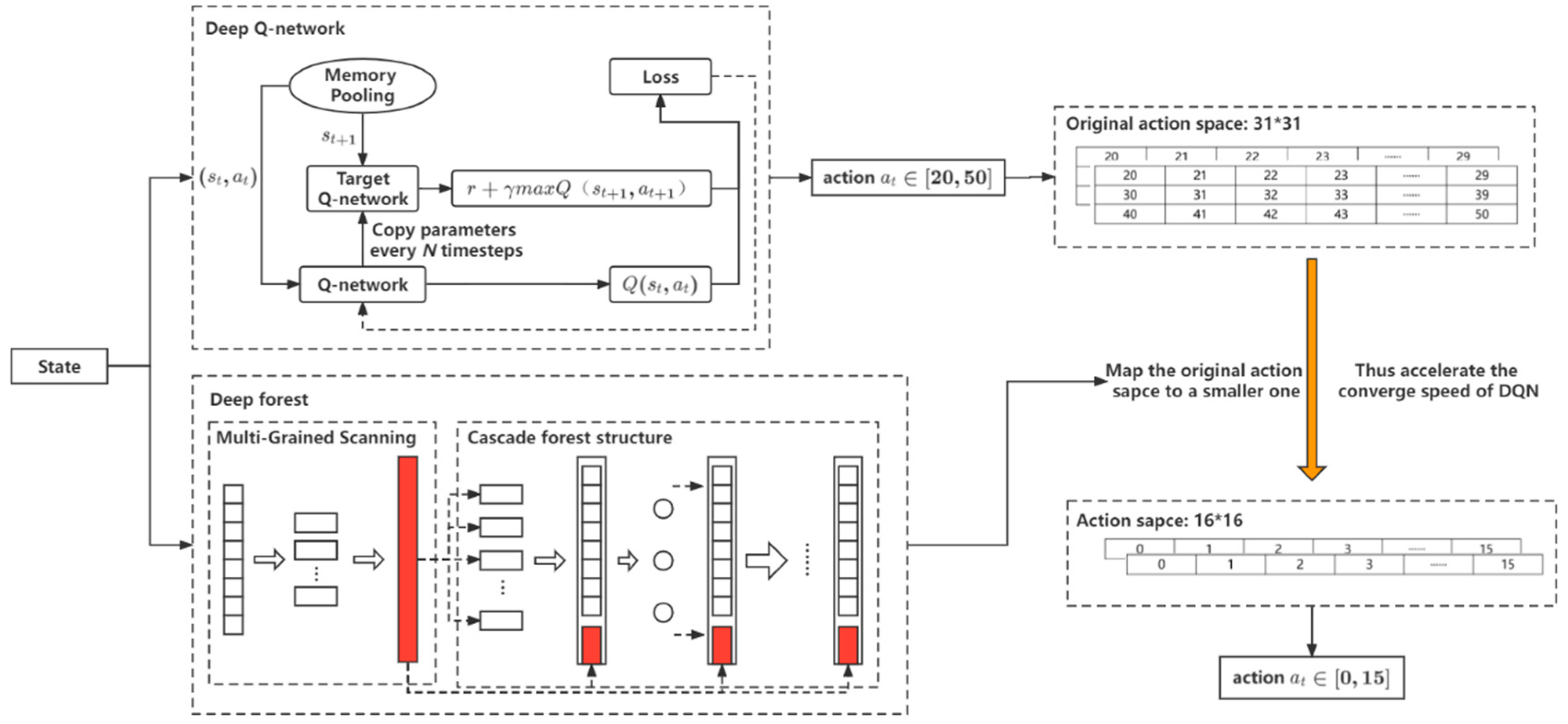
• We extended our previously proposed DF-DQN from the prediction problem to the control problem. The introduction of DF mapped the original DQN output action space into a new smaller action space, which could accelerate the convergence speed of DQN;
• We used DF-DQN to control a cooling water system in HVAC and to realize energy savings from the early stage. A priori knowledge was introduced as a deep forest classifier, which can not only reduce the action space, but also reduce the exploration of the agent. The experimental results show that DF-DQN can save energy from the first year, while DQN can achieve similar energy saving from the third year;
• We verified the performance of DF-DQN in an environment based on the modeling of a real cooling water system, so as to ensure the credibility of DF-DQN. The data that DF-DQN and other compared methods used were collected from a real-world system, and the simulation environment was built based on this system. The code and the experimental data are available at: https://github.com/H-Phoebe/DF-DQN-for-energy-saving-control (accessed on 20 August 2022).

2. Related Works

In recent years, more and more researchers have tried to solve practical problems with RL methods. In the applications of the HVAC system, the complexity and lag of the HVAC system directly lead to an increase in modeling cost, while RL can provide model-free control and have good control performance. However, RL generally takes a relatively long time to learn a better control policy, and this process may lead to some unnecessary energy wastage and cost increases, so some researchers try to avoid this wastage by speeding up the convergence of RL algorithms, which can achieve more energy saving at the same time.

Applications of RL in HVAC. Lork et al. [10] used Q-learning to achieve a balance between comfort and energy savings in rooms. They used a Bayesian convolutional neural network combined with data from all rooms to construct a temperature and air conditioning power prediction model to reduce uncertainty. This model was then adapted to individual rooms and the temperature set point was controlled using Q-learning. Qiu et al. [8] used Q-learning to obtain optimal control of the cooling water system in HVAC, wherein the RL controller can save 11% of the system energy, more than the 7% saved by the local feedback controller. Ahn et al. [11] used DQN to achieve a model-free optimal control policy in HVAC and the results proved that DQN can reduce energy consumption, and provided model-free optimal control. Brandi et al. [12] used DQN to control the water supply temperature set point of the heating system terminal unit, which can achieve a heating energy saving ranging between 5% and 12%. Yan et al. [13] applied DDPG to generate an optimal control policy for a multi-zone residential HVAC system, which can greatly reduce energy consumption while ensuring comfort. In addition, the DDPG-trained agent can intelligently balance different optimization objectives with generalization ability and adaptability to unknown environments. Ding et al. [14] used RL algorithms to control the indoor temperature of a residential HVAC system, which can achieve energy conservation while maintaining indoor thermal comfort. Qiu et al. [15] used three multi-agent RL algorithms to control the condenser system in HVAC. The experimental results showed that the interaction multi-agent RL algorithm can achieve better energy-saving effects compared to the other two algorithms. Amasyali et al. [16] used the deep RL controller to control the power cost of electric water heaters in residential buildings. The experimental results showed that this method does not cause discomfort to users, and can save 19–35% of the power cost compared with the baseline control.

Improve RL convergence speed. In engineering applications, the convergence time of RL methods may be several months or even years, which directly leads to an increase in cost. Therefore, some researchers have tried to shorten this time to reduce the cost of practical applications. Li et al. [17] controlled the HVAC system in order to control energy consumption and ensure comfort, and they put forward multi-grid Q-learning to solve the problem of slow convergence rate in RL. Yu [18] et al. developed an exploration policy for the RL controller using a priori knowledge, which can guide the RL controller to explore the action space, thus reducing the training time. Fu et al. [19] used a multi-agent RL to realize the collaborative control optimization of multiple devices in the HVAC system. The experimental results showed that the method converges faster than single-agent RL method. In [20], the authors mention that adding a priori knowledge can help the RL controller reduce training time.

3. Preliminaries

3.1. MDP

RL, as a class of control techniques in machine learning, has been explored for its potential in HVAC systems. In RL, the problem can often be considered as a sequential decision-making case, and the agent can learn by interacting with the environment directly, as shown in Figure 1.

Markov’s decision process (MDP), a classical formalization of sequential decision-making, is often used to model RL problems. An MDP can be defined as a tuple $\langle S, A, T, R, \gamma \rangle$, where $S$ is the collection of states, $A$ is the collection of actions, $T$ is a transition function, $R$ is an immediate reward function, and $\gamma$ is a discount factor. In the interactive process, for some states, the agent can select an action to act on the environment, and receive a scalar reward and a next state [21]. The final goal of RL is to maximize a cumulative numerical reward, $R_t$, as is shown in Equation (1).

$$R_t={\displaystyle \sum }_{k=0}^{\infty }{\gamma }^k{r}_{t+k+1}$$

(1)

where $\gamma \in \left[0, 1\right]$ is the discount factor, $k$ represents $k$ time steps after time step t, and $r_{t+k+1}$ represents the immediate reward of the corresponding time step. The agent selects an action $a ϵ A$ by policy $\pi$, then the agent moves to the next state $s_{t+1}$, then the agent obtains the immediate reward $r_{t+1}$ from the environment. In RL, the action value $Q$ is used to represent the exception of a cumulative discounted reward, which is starting from state $s$ and taking action $a$. The action value $Q$ is shown in Equation (2).

$$Q_{\pi }\left(s,a\right)=E_{\pi }\left[{\displaystyle \sum }_{k=0}^{\infty }{\gamma }^k{R}_{t+k+1}|s_t=s, a_t=a\right]$$

(2)

The optimal policy ${\pi }_{\ast }$ can be achieved by evaluating the action value function:

$$Q_{\ast }\left(s,a\right)=\max Q_{\pi }\left(s,a\right)=E\left[R_{t+1}+\gamma \underset{a^{\prime }}{\max }{Q}_{\ast }\left(s_{t+1}, a^{\prime }\right)|s_t=s, a_t=a\right]$$

(3)

Finally, the optimal policy ${\pi }_{\ast }$ can be obtained.

3.2. Deep Forest

Deep forest (DF) [22] is a decision tree ensemble approach and can be applied to classification tasks. DF can obtain good performance in most cases, even with different data in different domains, which mainly benefits from two techniques, namely multi-grained scanning and the cascade forest structure.

Multi-grained scanning uses sliding windows of various sizes for sampling to obtain more feature sub-samples, so as to obtain more and richer feature relationships. Then, a certain amount of the random forest and cascade forest are trained with the obtained feature sub-samples to obtain the feature vector.

The cascade forest structure is used to enhance the representation learning ability of DF. In a cascade forest, each level receives the characteristic information processed by the previous level, then the processing results in inputs, which are then output to the next level. The first level’s input of a cascade forest is the feature vector after multi-granularity scanning transformation. The final prediction result is obtained at the last level and expressed as an aggregate value.

In addition, the training process of the deep forest is efficient, and it can operate normally even if the training data scale is small. The structure of DF is shown in Figure 2.

3.3. DQN

Traditional methods in RL, such as SARSA and Q-learning, can effectively solve problems with a small state and action space by establishing Q-table. However, when the state space is large enough or continuous, such as practical problems in HVAC, these methods may fail to achieve a control policy. DQN, a method proposed by Google’s DeepMind in 2015 [23], has been applied in HVAC controls in recent years. Different from SARSA and Q-learning, DQN can solve problems with large or continuous state space [24], mainly benefiting from its two specific techniques.

Firstly, DQN uses the mechanism of experience replay to eliminate the correlation of network inputs. This means storing the transfer samples $\left(s,a,r,s^{\prime }\right)$ while the agent interacts with the environment and samples randomly to train the agent. Secondly, there are two networks in DQN, where one is the Q-network, and the other is the target network. These two networks have the same structure, but have different parameters. The Q-network outputs the current Q value, and the target network outputs the target Q value. After some iterations, the parameters of the Q-network are copied to the target network. The loss function is shown in Equation (4).

$$L\left({\theta }_i\right)=E\left[{\left(r+\gamma \underset{a^{\prime }}{\max }Q(s^{\prime }, a^{\prime } |{\theta }_i^{-})-Q(s, a |{\theta }_i)\right)}^2\right]$$

(4)

where $a^{\prime }$ is the action selected in state $s^{\prime }$, and ${\theta }_i$ and ${\theta }_i^{-}$ are the parameters of Q-network and target network, respectively.

4. Environment and Modeling

4.1. Cooling Water System Layout

In this paper, we tried to control the cooling water system to reduce the energy consumption of the HVAC system. The cooling water system is an important part of HVAC, including chillers, cooling water pumps, cooling towers, and some other necessary equipment. To achieve the goal of energy saving, it is important to enable this equipment to be controlled more efficiently. In another word, we should try to find an optimal policy to coordinate this equipment. Based on a real application, we constructed a cooling water system platform, which contained four chillers, three cooling water pumps, and seven cooling towers (the same type of equipment has the same settings), as shown in Figure 3.

To measure the effect of the control policy, we adopted the system coefficient of performance (COP), which is often used to measure the energy-saving performance of HVAC systems. The system COP is defined in Equation (5).

$$COP=\frac{C{L}_{system}}{\sum P_{chillers}+\sum P_{towers}+\sum P_{pumps}}$$

(5)

where $\sum P_{chillers}$ is the total power of all chillers (kW), $\sum P_{towers}$ is the total power of all cooling towers (kW), and $\sum P_{pumps}$ is the total power of all cooling water pumps (kW). $C{L}_{system}$ is the system cooling load, which is defined in Equation (6).

$$C{L}_{system}=C_p\times \rho \times F_{chw}\times \left(T_{chwr}-T_{chws}\right)÷3600 \mathrm{s}/\mathrm{h}$$

(6)

where $C_p$ is the specific heat capacity of water ($4.2 \mathrm{kJ}/\left(\mathrm{kg}·\mathrm{K}\right)$), $\rho$ is the water density ($1000 \mathrm{kg}/{\mathrm{m}}^3$), $F_{chw}$ is the chilled water flowrate (${\mathrm{m}}^3/\mathrm{h}$), $T_{chwr}$ is the inlet chilled water temperature of chillers (°C), and $T_{chws}$ is the outlet chilled water temperature of chillers (°C).

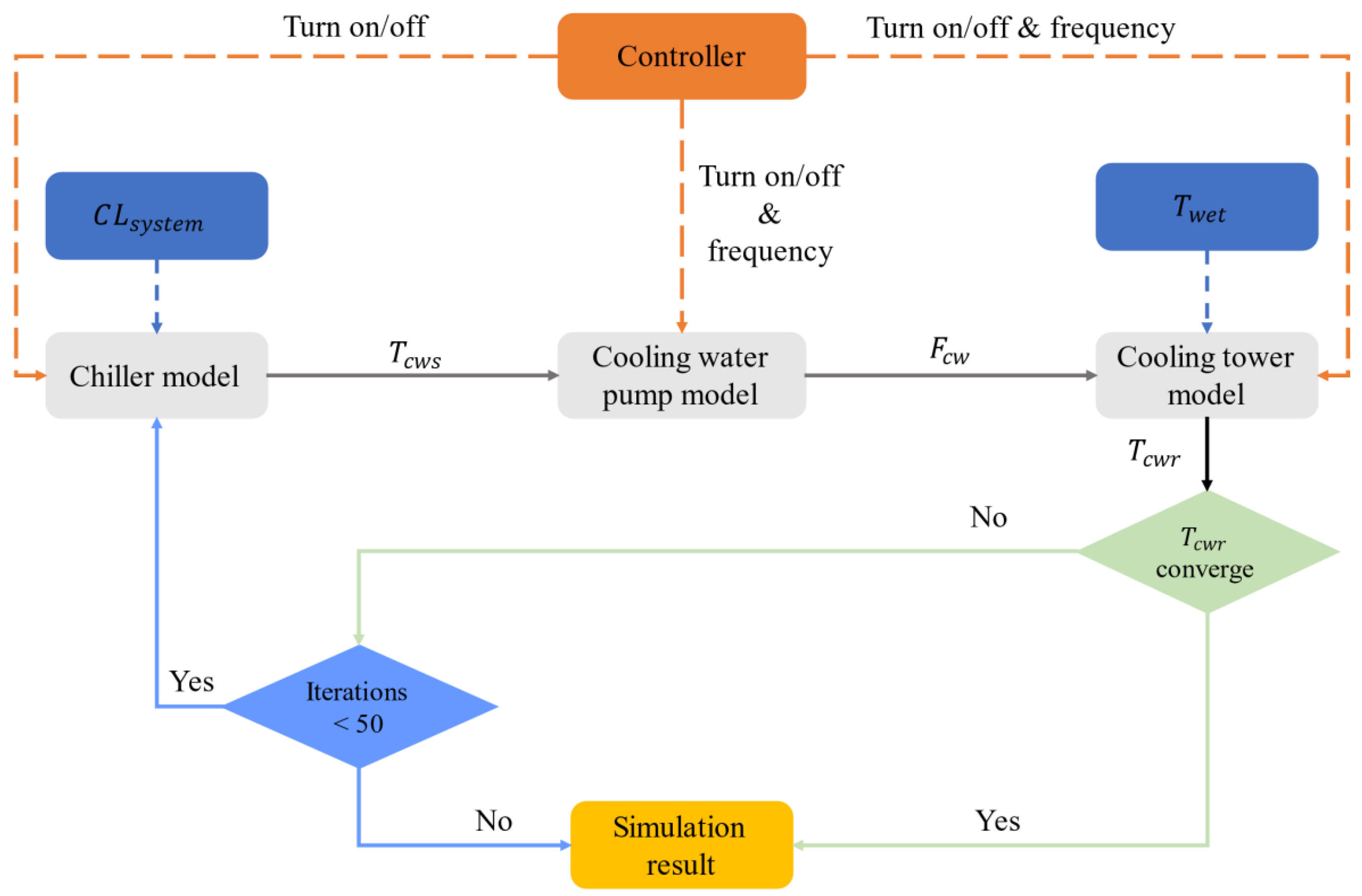
4.2. System Simulation Modeling

For the system simulation, some real data and parameters were collected, but some others could not be achieved directly, so we tried to use the regression method to attain them.

We regressed the chiller model with historical data, which could be used to attain the chiller’s COP, and further, we calculated the chiller’s power, as shown in Equation (7).

$$P_{chiller}=CL / CO{P}_{chiller}$$

(7)

where $CO{P}_{chiller}$ is obtained by Equation (8).

$$CO{P}_{chiller}=chiller model\left(CL, T_{cwr}, T_{chws}, F_{chw}\right)$$

(8)

where $T_{cwr}$ is the inlet cooling water temperature of chillers (°C). Some other related parameters are shown in Equations (9)–(11) [8].

$$T_{cws}=T_{cwr}+\left(P_{chiller}+CL\right)÷\frac{C_p\times F_{cw}\times \rho }{3600 \mathrm{s}/\mathrm{h}}$$

(9)

$$T_{chws}=\max \left[T_{chws}{}_{set}, T_{chwr}^{\prime }-CC÷\frac{C_p\times F_{chw}\times \rho }{3600 \mathrm{s}/\mathrm{h}}\right]$$

(10)

$$T_{chwr}=T_{chws}+CL ÷\frac{C_p\times F_{chw}\times \rho }{3600 \mathrm{s}/\mathrm{h}}$$

(11)

where $T_{{chws}_{set}}$ is the $T_{chws}$ set point of a chiller, $T_{chws}^{\prime }$ is the $T_{chws}$ of last time step, $F_{cw}$ is the cooling water flowrate (${\mathrm{m}}^3/\mathrm{h}$), and CC is the chiller cooling capacity.

The power of the cooling water pump model is calculated by Equations (12) and (13).

$$K=\frac{f_{pum{p}_{actual}}}{f_{pum{p}_{rated}}}$$

(12)

$$P_{pump}=a+b\times K+c\times K^2+d\times K^3$$

(13)

where $f_{pum{p}_{actual}}$ and $f_{pum{p}_{rated}}$ are the actual running frequency and rated running frequency of the real cooling water pump, and $a, b, c, d$ are determined by the regression of historical data.

The cooling tower model is defined as Equations (14) and (15).

$$P_{tower}=a+b\times f_{{tower}_{actual}}+c\times {f_{{tower}_{actual}}}^2+d\times {f_{{tower}_{actual}}}^3$$

(14)

$$T_{cwr}=tower model\left(T_{cws}, f_{towe{r}_{actual}}, T_{wb}, F_{cw}\right)$$

(15)

In Equation (14), $f_{towe{r}_{actual}}$ is the actual running frequency of cooling tower, $a,b,c,d$ are determined by the regression of historical data. In Equation (15), $T_{cwr}$ is the inlet cooling water temperature of chillers (°C), $T_{cws}$ is the outlet cooling water temperature of chillers (°C), $T_{wb}$ is ambient wet-bulb temperature (°C), and $F_{cw}$ is the cooling water flowrate (${\mathrm{m}}^3/\mathrm{h}$).

For each model, we randomly selected 80% of the collected data set for training and 20% of the data for testing, using MAPE (mean absolute percentage error) and CVRMSE (the coefficient of variation of the root mean square error) as the error metrics to evaluate the accuracy of the models. All models had a MAPE of less than 5% and CVRMSE of less than 10%, which indicates that the accuracy of each model was within the acceptable range.

The controller controlled the on and off states of this equipment and the operating frequency. An iterative process was as follows: Firstly, $T_{cws}$ was obtained from the $CL$ and the switching state of the chiller model; then, $F_{cw}$ was obtained by combining the operating frequency and $T_{cws}$; finally, $T_{cwr}$ was obtained by combining the cooling tower model with $F_{cw}$ and the $T_{wet}$. All the parameters were iterated until $T_{cwr}$ converged (i.e., the difference of $T_{cwr}$ between two successive iterations was less than 0.1 °C). If the $T_{cwr}$ did not converge within 50 iterations, the last result of $T_{cwr}$ was adopted and the iteration was stopped [8]. The specific process is shown in Figure 4.

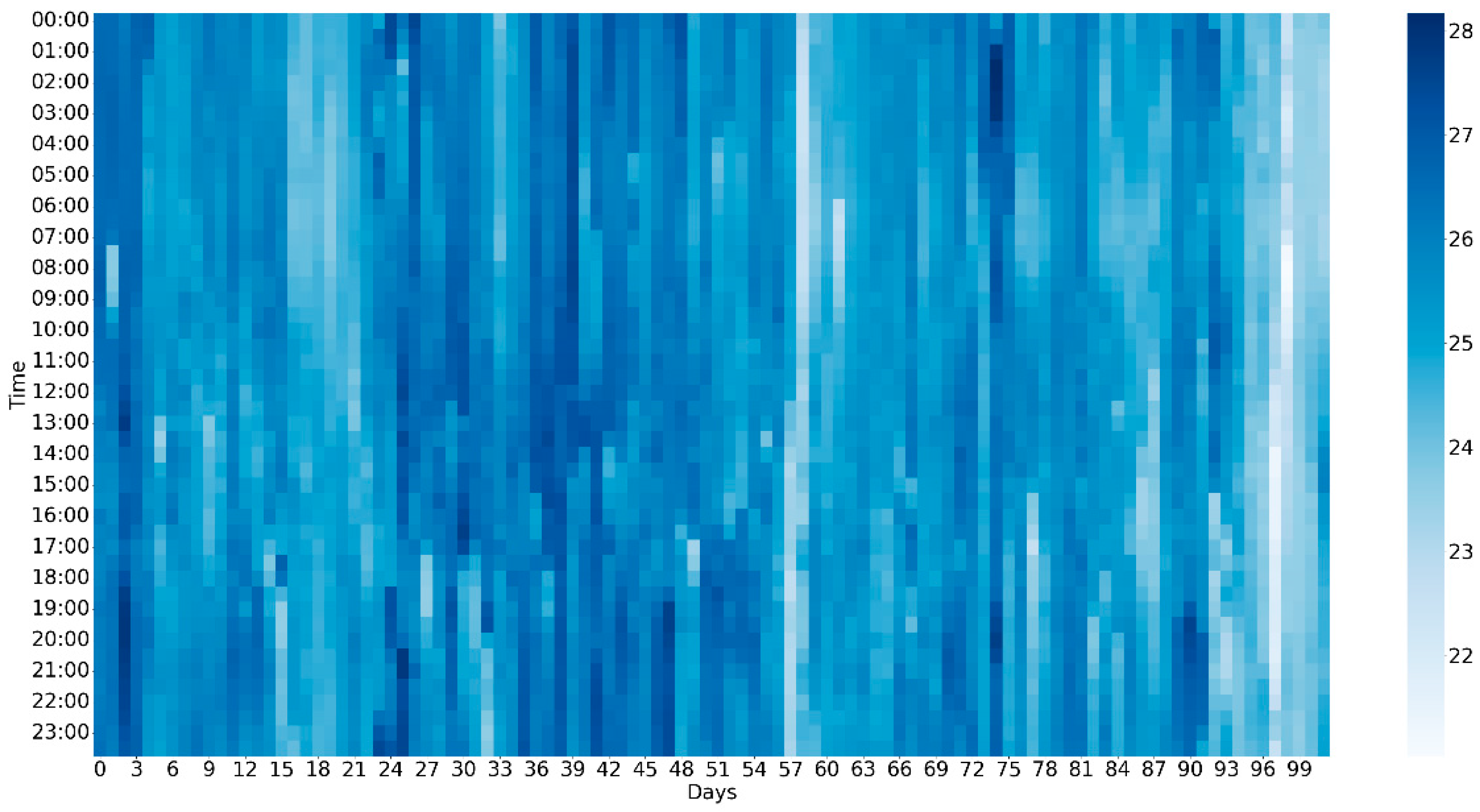
4.3. Data Collection

We used the data collected from the actual system to verify our proposed method. The details of this actual system corresponded with our simulation environment.

We collected real data from 1 July 2021 to 10 October 2021, 102 days in total, where the sample interval was half an hour. The $CL$ is shown in Figure 5, and the wet-bulb temperature is shown in Figure 6.

As shown in Figure 5 and Figure 6, the darker the color, the greater the value of $CL$ and the wet-bulb temperature ($T_{wet}$). From Figure 5, we can find that the main cooling demand of the system was concentrated between 6:00 and 23:00 every day.

5. Methodology

5.1. MDP Modeling

Using RL methods for control problem requires MDP modeling of the environment. The details of the modeling are represented as follows:

(a)

State

In this paper, we took the combination of ambient the wet-bulb temperature ($T_{wet}$) and system cooling load ($C{L}_{system}$) as state. There were two reasons for using these two variables:

(1)

The operation of the system has no influence of these variables;

(2)

$C{L}_{system}$ is a component factor of COP, which is related to the operation of cooling water system.

(b)

Action

In this paper, operating frequencies of cooling tower fans and cooling water pumps were taken as the action (e.g.,$\left[pump\_action:35\mathrm{hz},tower\_action:35\mathrm{hz}\right]$). In addition, the action was discretized and the control accuracy was 1 hz. In order to protect the equipment, the action needed to be limited within a reasonable range. We limited the action frequency within [20, 50] for both the cooling tower and cooling water pump, so there were 31 actions in total for each one.

(c)

Reward

COP was taken as the reward in this paper. In the case of the same $C{L}_{sysytem}$, the higher the COP value is, the sum of power is the lowest, which reflects the purpose of energy saving. The reward is shown in Equation (16).

$$Reward=COP=\frac{C{L}_{system}}{\sum P_{chillers}+\sum P_{towers}+\sum P_{pumps}}$$

(16)

5.2. DF-DQN for Control

Figure 7 depicts the overall framework of DF-DQN for control in cooling water system. Firstly, we labeled the collected state data, including cooling load and wet-bulb temperature, according to the a priori knowledge. The label was the running frequency of the equipment more or less than the value of the base number under this state. If the operating frequency of the equipment under this state was less than base number, the label was ‘0’; otherwise, the label was ‘1’. The labeled state data were used to train the deep forest classification model, of which 80% was used for training and 20% was used to test the accuracy of the trained model.

After training, the DF classification model can output a label for the new state, which represents the relationship between the actual frequency of equipment operation and the base number, and this label can be converted into a sign to shrink the action space thereafter. Figure 8 gives more details.

Secondly, we obtained the relationship between the actual frequency of the equipment operation and base number under some states, namely the sign. We also needed the difference between the operating frequency of the actual equipment and the base number. In this part, we trained DQN agent, which output an action $a_t^{\prime }$, the absolute value of the difference between the true action and base number, namely $\Delta$.

At last, according to the actual data we collected, the DF classifier output a positive sign or negative sign (‘+’ & ‘−’), and DQN output $\Delta$. Based on sign, $\Delta$, and base number, we could obtain the actual equipment running frequency, namely action $a_t$. The actual action is calculated according to Equations (17) and (18).

$$Sign=D{F}_{classifier}\left(state\right)$$

(17)

$$a_t=bas{e}_{number}+Sign\left(a_t^{\prime }\right)$$

(18)

where $sign$ is output by DF, $a_t^{\prime }$ is output by DQN in DF-DQN.

5.3. Theoretical Analysis of Shrink Action

The DF classifier labeled each state. It could replace the original action space with a smaller action space combined with the label, so as to realize the reduction of the action space.

Owing to the introduction of DF in DQN, the original action space of each equipment was reduced from 31 to 16, so the original combined action pace was reduced from 31 × 31 to 16 × 16. Therefore, the action space of each equipment was reduced by nearly half, while the combined action of the two equipment reduced the action space by nearly 3/4 with the increase in equipment types. The introduction of DF could make the combined action space decrease exponentially. Figure 9 presents more details.

Theoretically, if DF can divide each action into M categories with the same number, and the final combined actions include N kinds, the reduced action space of DF-DQN can follow Equation (19).

$$\frac{{\left(Action space\right)}_{DF-DQN}}{Original action space} \approx {\left(\frac{1}{M}\right)}^N$$

(19)

Based on the above analysis, when dealing with the problem with large action space or multiple action combinations, DF can significantly shrink the scale of the original action space, which can reduce the complexity of the problem to a certain extent finally.

In this paper, $M=2$, $N=2$, so the combined action of the two equipment was shrunk into about 1/4 of the original action space.

5.4. DF-DQN Algorithm

The details of DF-DQN for the cooling water system is shown in Algorithm 1.

Algorithm 1. DF-DQN for cooling water system

Initialize replay memory $D$ to capacity $N$ Initialize action value function $Q$ with random weights $\theta$ Detect and replace outliers in training set Split the training set (80% for training, 20% for testing) Train the deep forest classifier $F$ For episode = 1, M do  Attain initial state $s_t$ of the cooling water system  For t = 1, T do   Select a random action $a_t^{\prime }$ with probability $\epsilon$, otherwise $a_t^{\prime }=\max Q\left(s_t, a; \theta \right)$   Attain positive or negative sign through $F$   Combine base number, sign (‘+’ or ‘−’), $a_t^{\prime }$ to derive $a_t$(the true running frequency of cooling water system)   Execute action $a_t$ in cooling water system   Observe reward $r_t$ and state $s_{t+1}$ from the simulation system   Store transition ($s_t, a_t^{\prime }, r_t, s_{t+1}$) in $D$   Sample random minibatch of transitions ($s_j, a_j^{\prime }, r_j, s_{j+1}$) from $D$   Set $y_j=\{\begin{array}{cc}\hfill r_j\hfill & for terminal state s_{t+1}\hfill \\ \hfill r_j+\gamma \underset{a^{\prime }}{\max }Q\left(s_{j+1}, a^{\prime }; \theta \right)\hfill & otherwise\hfill \end{array}$   Update Q function using ${\left(y_i-Q\left(s_j, a_j; \theta \right)\right)}^2$   Copy parameters every $J$ steps   Update state $s_t\leftarrow s_{t+1}$  End for End for

6. Experiment and Result

To verify the performance of DF-DQN, we compared it with three other benchmark methods. In addition, we presented some experiments about the effect of DF accuracy on the performance of DF-DQN.

6.1. Compare Methods

• DF-DQN: DF-DQN is the method we proposed before [25], which has been used to solve prediction problem. We extended DF-DQN to control problems in this paper;
• DQN: In this paper, DQN and DF-DQN share the same parameter settings in the DQN part. For the cooling water system, the action space was small and discrete, and its state space was large enough, so usually DQN can provide a good control policy according to paper [24];
• Baseline control: The PID control was selected as the baseline method, which is often used in real HVAC control applications. This method selects the action by approaching the difference between $T_{cws}$ and $T_{cwr}$. We took the baseline control method for comparison because it is the original control method in this system;
• Model-based control: The model-based control is the best method among all methods, and can select the best action in each situation, but this method is heavily dependent on the model. In this paper, we traversed the best action in each state as the model-based control. Actually, it is often impossible to deploy the model-based control method in real applications, but in this paper, based on our simulation model, the model-based control method provided the best policy. We used the model-based control method for comparison because it has the best control performance of all methods in this system.

6.2. Parameters Setting

We used DF-DQN and three other methods to control this system for comparison, including DQN, a baseline control, and a model-based control.

The agent in DF-DQN took the $\epsilon -greedy$ policy to select the action. At the beginning, we ensured the agent could explore the environment as much as possible, so we set ${\epsilon }_{inital}=1$. We used a liner decay during the process, and set $\Delta \epsilon =0.0001$, ${\epsilon }_{min}=0.01$. In order to make the agent take more focus on the current COP, we set $\gamma =0.01$. The agent’s policy network and target network were both composed of two hidden layers. The minibatch was set to 32. The capacity of memory pooling ($Memor{y}_{capacity}$) was set to 1000, and we set $C_{step}$ (Copy steps) to 100, $C_{step}=100$. The learning rate was set to 0.01, $\alpha =0.01$. All parameters are shown in

Table 1. Parameters of DF-DQN and DQN.

Parameters	Value
${\epsilon }_{inital}$	1
$\Delta \epsilon$	0.0001
${\epsilon }_{min}$	0.01
$\gamma$	0.01
$Memor{y}_{capacity}$	1000
$C_{step}$	100
$\alpha$	0.01

.

In this system, the equipment contained chillers, cooling water pumps, and cooling towers. We used RL to control the cooling water pumps and cooling towers. As for the chillers, we used a sequence control [26] to reduce unnecessary refrigerating capacity, which can protect chillers at the same time. The workflow of this system is shown in Appendix A.

6.3. Experimental Result

In this paper, we used the model-based control to attain the best action in each state, so that we could attain the label of the cooling water pump and cooling tower’s action under each state. We used DF for two classifications to judge whether the frequency of the cooling water pump and cooling tower was more or less than the base number in each state. If it was more than the base number, we labeled it as 1 (represent ‘+’); otherwise, we labeled it as 0 (represent ‘−’). The accuracy of DF can reach 97.319% and 99.694%. DF-DQN combined DF and DQN, where DF output sign ‘+’ or ‘−’, and DQN of DF-DQN output $\Delta$, and then we combined them with base number to attain the final action of the cooling water pump and cooling tower.

Cumulative reward in an episode was taken to prove the convergence of DF-DQN. With the increase in episode, when the value of cumulative reward fluctuated less, we believe that the method converged. One of the comparison methods, DQN, also used the same method. The reward was defined by Equation (16), namely COP, and the higher reward not only conveyed that it had better converge, but also represented that the method had better energy-saving performance.

We explain the experimental results from two aspects: one is the influence of DF’s accuracy on DF-DQN, and the other is control performance of DF-DQN.

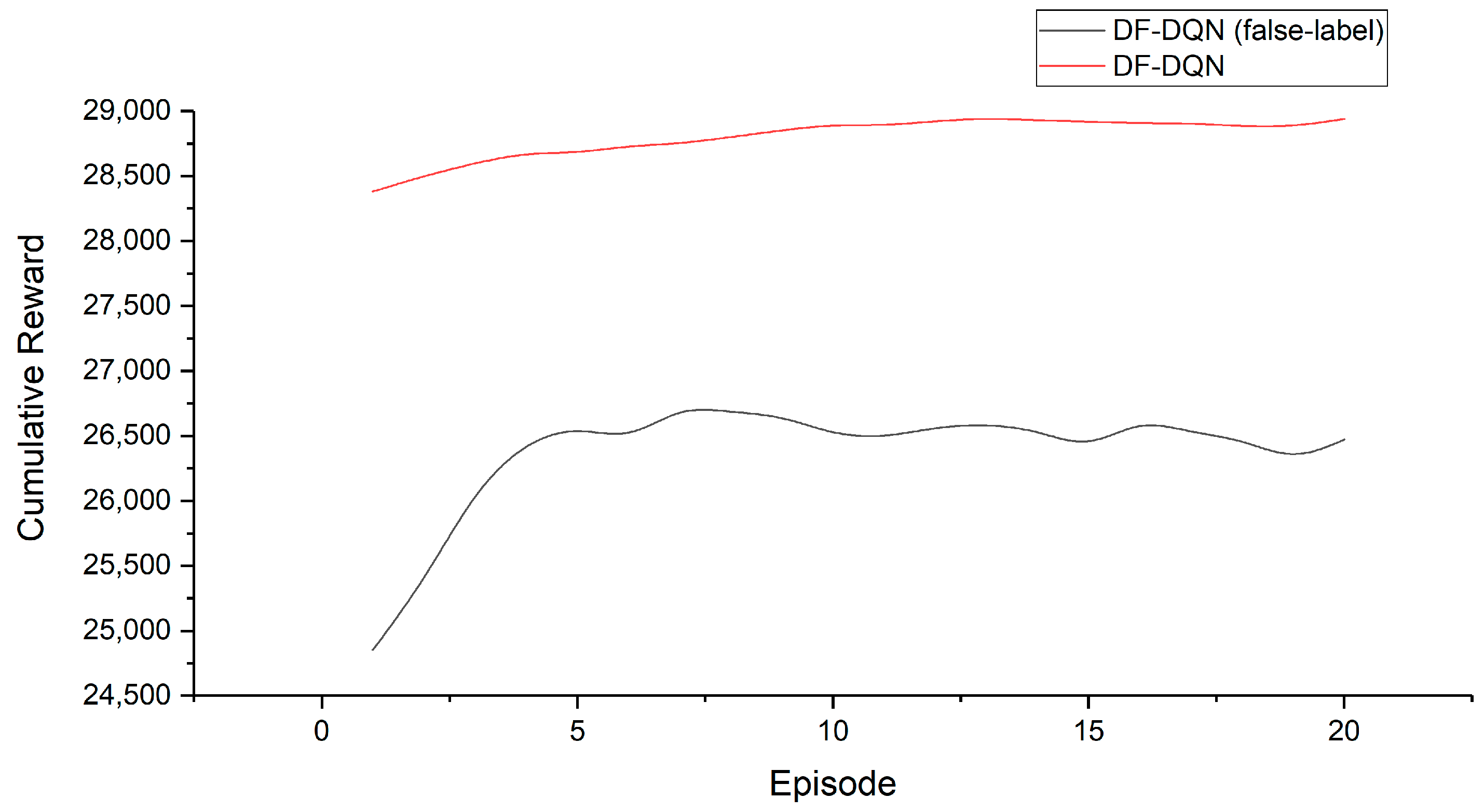
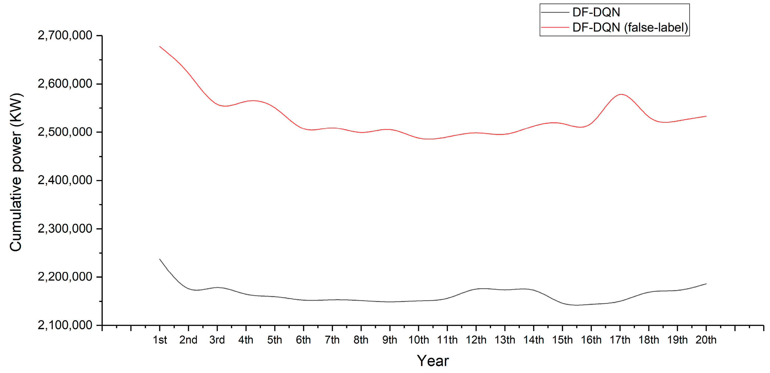
6.3.1. Influence of DF’s Accuracy on DF-DQN

The accuracy of DF affected the performance of DF-DQN. In order to better explain the influence of DF accuracy on the performance of DF-DQN, we made a test with a low accuracy case. We used DF-DQN (false label) and DF-DQN to control the system for 20 years in our simulation environment. We randomly generated labels to replace the original labels that DF generated, so that we could analyze the impact of DF accuracy on the performance of DF-DQN. The accuracy of the randomly generated labels was 50% of the original labels. We compared the experimental results of DF-DQN (false label) with the DF-DQN from three aspects: COP, cumulative power, and energy-saving effect.

Before comparison, we needed to ensure that both methods could converge. The convergence of the two methods is shown in Figure 10, where one episode in the training process is one year.

DF-DQN (false label) and DF-DQN both converged at last. Although the wrong label was used, DQN still learned the control policy under the wrong labels and converged. However, the cumulative reward of DF-DQN was higher than that of DF-DQN (false label) on the whole, which also reflected the better performance of DF-DQN. In addition, the performance of DF-DQN (false label) decreased a lot due to the false labels.

As shown in Figure 11, the COP of DF-DQN (false label) was lower than that of DF-DQN in 20 years, which indicates that the control performance of DF-DQN (false label) was worse than that of DF-DQN in each year, and the energy-saving effect decreased accordingly, which also can be found in the cumulative power comparison in Figure 12.

We compared the energy-saving effect of these two methods, and used the baseline control method of the system as a benchmark. The partial energy-saving effect comparison can be found in

Table 2. Partial energy-saving effect comparison result.

Energy Saving (Compared to Baseline Control)
Year	DF-DQN	DF-DQN (False Label)
1st	8.074%	−10.022%
2nd	11.337%	−8.037%
3rd	10.086%	−4.224%
5th	11.157%	−5.191%
10th	11.580%	−1.934%
15th	12.168%	−3.754%
20th	10.177%	−4.094%
Average (20 years)	11.035%	−4.104%

.

Regardless of the comparison of COP, the cumulative power, or the energy-saving effect, DF-DQN (false label) was worse than DF-DQN. The direct reason for this result was the wrong labels. From the comparison result, we found that the accuracy of DF directly affected the performance of DF-DQN, and the low accuracy of DF led to a decrease in the performance of DF-DQN. Therefore, for DF-DQN control in this problem, it was crucial to improve the accuracy of DF as much as possible.

6.3.2. Performance of DF-DQN Compared with DQN, Baseline Control, and Model-Based Control

DF-DQN and DQN both converged at last, but in the beginning episodes, DF-DQN achieved a higher cumulative reward. The difference between DF-DQN and DQN can be found in Figure 13 more clearly.

As shown in Figure 13, the cumulative reward of DF-DQN was much greater than that of DQN before the fifth episode, which reflects that the control performance of DF-DQN was much better than DQN in the early stage. After the fifth episode, DQN outperformed DF-DQN, which was due to the accuracy of DF. However, the performance of DF-DQN was almost approaching DQN.

In order to compare the performance of the baseline control method, DQN, DF-DQN, and the model-based control method, we used them to control the system for 20 years in our simulation environment. We compared their performance in three aspects: the COP, the cumulative power, and the energy-saving effect.

(a)

COP

The COP is shown in Figure 14. The model-based control method was the best method among these methods in theory, and its COP was the highest in practice. The baseline control method is a relatively poor control method compared with others, and its COP was the lowest in most of the years.

From Figure 14, we found that the COP obtained by DQN and DF-DQN was gradually becoming higher, indicating that their energy-saving effect was gradually becoming better, which is just as we have mentioned before, and the higher system COP, the better the energy-saving performance. The distribution of COP in the first year reflects that the control effect of DQN was much worse than that of DF-DQN, but it gradually became better in the later years. The COP reflected its better energy-saving performance to a certain extent, but not absolutely. In addition, the minimum COP obtained by DQN and DF-DQN was relatively small, which was due to the poorly selected actions in a few states.

As for DQN, its COP was less than the baseline control method in the first year, and the distribution of COP in the first year was also relatively scattered, but in the second year, the distribution of COP became concentrated, and its COP was more than the baseline control method, which meant that DQN’s control performance became better in the second year. Finally, DQN’s COP became stable, which means that the control policy of DQN was becoming stable and convergent.

In contrast with DQN, DF-DQN’s COP was between the baseline control method and model-based control method from the first year and this trend remained in the following 20 years, which reflected that DF-DQN can obtain a better control effect from the beginning, and the control effect was better than DQN in the early stage. Moreover, the performance of DF-DQN was more stable than DQN in 20 years.

The performance of DQN was not good in the early stage, and its COP was not between the baseline control method and model-based control method until the policy converged. In contrast, DF-DQN met this condition not only after the convergence of the control policy, but also from the very beginning, which reflected that DF-DQN converged faster than DQN, and had a better performance than DQN in the early stage.

(b)

Cumulative power

In order to intuitively analyze the energy-saving effect of these four methods, we compared the annual cumulative power under these four methods’ control policies, and the comparison results are shown in Figure 15.

In Figure 15, the model-based control method had the lowest cumulative power, which is consistent with the intuition. The baseline control method had a relatively poor energy-saving effect, and its cumulative power was relatively more than others.

The magnitude of DQN’s cumulative power was larger than that of the model-based control method and less than the baseline control method from the third year. In Figure 14, though DQN’s COP was more than the baseline control method in the second year, its cumulative power was still more than the baseline control method. In Figure 15, the cumulative power of DQN in the second year was less than that in the first year, and it continued to decrease until the fourth year, and then remained stable. As we mentioned in the previous part, the lower COP did not absolutely mean a better energy-saving effect, but from the experimental results, we found that the second year’s policy was better than the first year’s, which is also be conveyed in Figure 15.

DF-DQN’s cumulative power was much lower than the baseline control method from the first year, and this trend continued to decrease until the second year and then remained stable. In addition, DF-DQN’s cumulative power was also much less than DQN’s in the first three years, and after that, it almost approached DQN. It is obvious that DF-DQN can not only achieve a good energy-saving effect, but can also save energy from an early stage. Compared with DQN, the energy-saving effect of DF-DQN in the early stage was much better.

(c)

Energy saving

Taking the baseline control method as the benchmark, we compared the other three methods’ energy-saving effects in each year. The partial comparison results are represented in

Table 3. Partial comparison effect results.

Energy Saving (Compared to Baseline Control)
Year	DQN	DF-DQN	Model-Based Control
1st	−29.996%	8.074%	13.755%
2nd	−9.843%	11.337%	13.755%
3rd	0.798%	10.086%	13.755%
5th	12.195%	11.157%	13.755%
10th	11.908%	11.580%	13.755%
15th	11.461%	12.168%	13.755%
20th	12.094%	10.177%	13.755%
Average (20 years)	7.972%	11.035%	13.755%

, and the complete comparison results are shown in Appendix B.

There is no doubt that the model-based control method had the best energy-saving effect, reaching 13.775%. The energy-saving effect of DQN and DF-DQN both had a growth process before the convergence.

According to the experimental results, DQN could not achieve the goal of energy saving until the third year. In particular, in the first year, its energy-saving effect was 29.996% worse than the baseline control method. In the second year, DQN’s saving effect became much better than the first year, but was still 9.843% worse than the baseline control. Until the third year, DQN’s saving effect was 0.798% better than the baseline control method, and began to remain stable from the fourth year, and was able to achieve a 10–12% energy-saving effect each year. DQN’s energy-saving effect was not good in the early stage, but it became better and better with training. After 20 years control, its average energy-saving effect reaches 7.972%.

In contrast, DF-DQN could achieve the goal of energy saving from the first year, and remained with a 10–11% energy-saving effect. In the first year, it could achieve 8.074% better than the baseline control method, and kept becoming better in the second year, reaching 11.337%. After 20 years of the control, its average energy-saving effect reached about 11.035%.

DQN may have a better energy-saving effect in the later years, but it has to explore the environment before converging, which led to its worse performance in the early stage. Considering of the service life of the equipment, DF-DQN may have a better energy-saving effect than DQN in general, and our experimental results also proved this.

7. Conclusions and Future Work

In this paper, we extended DF-DQN from the prediction problem to the control problem, which was used to achieve the goal of energy saving with respect to the cooling water system control in HVAC. We compare its performance with DQN, baseline control method and the model-based control method. The experimental results show that since the a priori knowledge was introduced as a deep forest classifier, DF-DQN’s action space could be mapped to a smaller one. DF-DQN did not need to spend a lot of on exploring the environment, so it converged much faster than DQN, which is the main reason that DF-DQN shows a better performance in the early stage compared to DQN. In the latter stage, the performance of DF-DQN was always slightly worse than DQN, and the reason is that the DF classifier may have output some wrong labels in a few states, which directly affected the result and DF-DQN’s performance. Compared with the model-based control method, DF-DQN performed slightly worse in saving energy, but it did not require any complete system model, thus avoiding the unnecessary cost of modeling, which was valuable in the engineering practice.

DF-DQN had obvious energy-saving effects in the early stage and the overall energy-saving effect was also good, but its performance was directly affected by DF, which relied on historical data or expert experience. Thus, it is particularly important to train a DF classifier with excellent performance. DF-DQN has a good energy-saving effect in engineering applications, and is more practical than traditional RL methods, but it is not suitable for systems lacking historical data or expert experience. In addition, in this paper, we only considered two controllable equipment, but if more equipment need to be controlled, for example, more than 10 equipment, the performance of DF-DQN might decrease, which is limited by the DQN. Thus, for the future works, we will focus on following two aspects: (1) improving the accuracy of DF classifier or constructing a new classifier with higher accuracy, which could improve the final control performance in the current DF-DQN framework. (2) When more equipment of different types is involved, multi-agent reinforcement learning method can be adopted into the DF-DQN framework.

References

1. Cao, X.; Dai, X.; Liu, J. Building energy-consumption status worldwide and the state-of-the-art technologies for zero-energy buildings during the past decade. Energy Build. 2016, 128, 198–213. [Google Scholar] [CrossRef]
2. Taylor, S.T. Fundamentals of Design and Control of Central Chilled-Water Plants; ASHRAE Learning Institute: Atlanta, GA, USA, 2017. [Google Scholar]
3. Wang, S.; Ma, Z. Supervisory and optimal control of building HVAC systems: A review. HVAC&R Res. 2008, 14, 3–32. [Google Scholar] [CrossRef]
4. Wang, J.; Hou, J.; Chen, J.; Fu, Q.; Huang, G. Data mining approach for improving the optimal control of HVAC systems: An event-driven strategy. J. Build. Eng. 2021, 39, 102246. [Google Scholar] [CrossRef]
5. Gholamzadehmir, M.; Del Pero, C.; Buffa, S.; Fedrizzi, R.; Aste, N. Adaptive-predictive control strategy for HVAC systems in smart buildings–A review. Sustain. Cities Soc. 2020, 63, 102480. [Google Scholar] [CrossRef]
6. Zhu, N.; Shan, K.; Wang, S.; Sun, Y. An optimal control strategy with enhanced robustness for air-conditioning systems considering model and measurement uncertainties. Energy Build. 2013, 67, 540–550. [Google Scholar] [CrossRef]
7. Heo, Y.; Choudhary, R.; Augenbroe, G.A. Calibration of building energy models for retrofit analysis under uncertainty. Energy Build. 2012, 47, 550–560. [Google Scholar] [CrossRef]
8. Qiu, S.; Li, Z.; Li, Z.; Li, J.; Long, S.; Li, X. Model-free control method based on reinforcement learning for building cooling water systems: Validation by measured data-based simulation. Energy Build. 2020, 218, 110055. [Google Scholar] [CrossRef]
9. Claessens, B.J.; Vanhoudt, D.; Desmedt, J.; Ruelens, F. Model-free control of thermostatically controlled loads connected to a district heating network. Energy Build. 2018, 159, 1–10. [Google Scholar] [CrossRef] [Green Version]
10. Lork, C.; Li, W.T.; Qin, Y.; Zhou, Y.; Yuen, C.; Tushar, W.; Saha, T.K. An uncertainty-aware deep reinforcement learning framework for residential air conditioning energy management. Appl. Energy 2020, 276, 115426. [Google Scholar] [CrossRef]
11. Ahn, K.U.; Park, C.S. Application of deep Q-networks for model-free optimal control balancing between different HVAC systems. Sci. Technol. Built Environ. 2020, 26, 61–74. [Google Scholar] [CrossRef]
12. Brandi, S.; Piscitelli, M.S.; Martellacci, M.; Capozzoli, A. Deep reinforcement learning to optimise indoor temperature control and heating energy consumption in buildings. Energy Build. 2020, 224, 110225. [Google Scholar] [CrossRef]
13. Du, Y.; Zandi, H.; Kotevska, O.; Kurte, K.; Munk, J.; Amasyali, K.; Mckee, E.; Li, F. Intelligent multi-zone residential HVAC control strategy based on deep reinforcement learning. Appl. Energy 2021, 281, 116117. [Google Scholar] [CrossRef]
14. Ding, Z.; Fu, Q.; Chen, J.; Wu, H.; Lu, Y.; Hu, F. Energy-efficient control of thermal comfort in multi-zone residential HVAC via reinforcement learning. Connect. Sci. 2022, 34, 2364–2394. [Google Scholar] [CrossRef]
15. Qiu, S.; Li, Z.; Li, Z.; Wu, Q. Comparative Evaluation of Different Multi-Agent Reinforcement Learning Mechanisms in Condenser Water System Control. Buildings 2022, 12, 1092. [Google Scholar] [CrossRef]
16. Amasyali, K.; Munk, J.; Kurte, K.; Kuruganti, T.; Zandi, H. Deep reinforcement learning for autonomous water heater control. Buildings 2021, 11, 548. [Google Scholar] [CrossRef]
17. Li, B.; Xia, L. A multi-grid reinforcement learning method for energy conservation and comfort of HVAC in buildings. In Proceedings of the 2015 IEEE International Conference on Automation Science and Engineering (CASE), Gothenburg, Sweden, 24–28 August 2015; pp. 444–449. [Google Scholar] [CrossRef]
18. Yu, Z.; Yang, X.; Gao, F.; Huang, J.; Tu, R.; Cui, J. A Knowledge-based reinforcement learning control approach using deep Q network for cooling tower in HVAC systems. In Proceedings of the 2020 Chinese Automation Congress, CAC 2020, Shanghai, China, 6–8 November 2020; pp. 1721–1726. [Google Scholar] [CrossRef]
19. Fu, Q.; Chen, X.; Ma, S.; Fang, N.; Xing, B.; Chen, J. Optimal control method of HVAC based on multi-agent deep reinforcement learning. Energy Build. 2022, 270, 112284. [Google Scholar] [CrossRef]
20. Yang, L.; Nagy, Z.; Goffin, P.; Schlueter, A. Reinforcement learning for optimal control of low exergy buildings. Appl. Energy 2015, 156, 577–586. [Google Scholar] [CrossRef]
21. Sutton, R.; Barto, A. Reinforcement Learning: An Introduction, 2nd ed.; MIT Press: Cambridge, MA, USA; London, UK, 2018. [Google Scholar]
22. Zhou, Z.H.; Feng, J. Deep forest. Natl. Sci. Rev. 2019, 6, 74–86. [Google Scholar] [CrossRef]
23. Mnih, V.; Kavukcuoglu, K.; Silver, D.; Rusu, A.A.; Veness, J.; Bellemare, M.G.; Graves, A.; Riedmiller, M.; Fidjeland, A.K.; Ostrovski, G.; et al. Human-level control through deep reinforcement learning. Nature 2015, 518, 529–533. [Google Scholar] [CrossRef]
24. Fu, Q.; Han, Z.; Chen, J.; Lu, Y.; Wu, H.; Wang, Y. Applications of reinforcement learning for building energy efficiency control: A review. J. Build. Eng. 2022, 50, 104165. [Google Scholar] [CrossRef]
25. Fu, Q.; Li, K.; Chen, J.; Wang, J. A Novel Deep-forest-based DQN method for Building Energy Consumption Prediction. Buildings 2022, 12, 131. [Google Scholar] [CrossRef]
26. Li, Z.; Huang, G.; Sun, Y. Stochastic chiller sequencing control. Energy Build. 2014, 84, 203–213. [Google Scholar] [CrossRef]
Figure 1. The interaction progress between agents and environments in RL.
Buildings 12 01787 g001
Figure 2. Structure of deep forest.
Buildings 12 01787 g002
Figure 3. The layout of the cooling water system.
Buildings 12 01787 g003
Figure 4. Simulation process.
Buildings 12 01787 g004
Figure 5. The temporal distribution of the cooling load. The deeper the color, the heavier the load.
Buildings 12 01787 g005
Figure 6. The temporal distribution of the wet-bulb temperature. The deeper the color, the higher the temperature.
Buildings 12 01787 g006
Figure 7. Overall framework of DF-DQN for cooling water system.
Buildings 12 01787 g007
Figure 8. The process of training a DF classifier.
Buildings 12 01787 g008
Figure 9. DF reduce action space.
Buildings 12 01787 g009
Figure 10. Comparison of cumulative reward between DF-DQN (false label) and DF-DQN.
Buildings 12 01787 g010
Figure 11. Comparison of COP between DQN and DF-DQN.
Buildings 12 01787 g011
Figure 12. Comparison of cumulative power between DF-DQN and DF-DQN (false label).
Buildings 12 01787 g012
Figure 13. Comparison of cumulative reward between DQN and DF-DQN.
Buildings 12 01787 g013
Figure 14. COP comparison of each method.
Buildings 12 01787 g014
Figure 15. Cumulative power of each method in 20 years.
Buildings 12 01787 g015