Ensuring Earthquake-Proof Development in a Swiftly Developing Region through Neural Network Modeling of Earthquakes Using Nonlinear Spatial Variables

Abstract

Northern Pakistan, the center of major construction projects due to the commencement of the China Pakistan Economic Corridor, is among the most earthquake-prone regions globally owing to its tectonic settings. The area has experienced several devastating earthquakes in the past, and these earthquakes pose a severe threat to infrastructure and life. Several researchers have previously utilized advanced tools such as Machine Learning (ML) and Deep Learning (DL) algorithms for earthquake predictions. This technological advancement helps with construction innovation, for instance, by designing earthquake-proof buildings. However, previous studies have focused mainly on temporal rather than spatial variables. The present study examines the impact of spatial variables to assess the performance of the different ML and DL algorithms for predicting the magnitude of short-term future earthquakes in North Pakistan. Two ML methods, namely Modular Neural Network (MNN) and Shallow Neural Network (SNN), and two DL methods, namely Recurrent Neural Network (RNN) and Deep Neural Network (DNN) algorithms, were used to meet the research objectives. The performance of the techniques was assessed using statistical measures, including accuracy, information gain analysis, sensitivity, specificity, and positive and negative predictive values. These metrics were used to evaluate the impact of including a new variable, Fault Density (FD), and the standard seismic variables in the predictions. The performance of the proposed models was examined for different patterns of variables and different classes of earthquakes. The accuracy of the models for the training data ranged from 73% to 89%, and the accuracy for the testing data ranged from 64% to 85%. The analysis outcomes demonstrated an improved performance when using an additional variable of FD for the earthquakes of low and high magnitudes, whereas the performance was less for moderate-magnitude earthquakes. DNN, and SNN models, performed relatively better than other models. The results provide valuable insights about the influence of the spatial variable. The outcome of the present study adds to the existing pool of knowledge about earthquake prediction, fostering a safer and more secure regional development plan involving innovative construction.

1. Introduction

Earthquakes are among the most perilous natural disasters, causing loss of life, serious calamities, and destruction of building infrastructures, resulting in both life and economic losses [1,2]. In the past two decades, earthquakes and tsunamis have naturally been the fatalist form of disasters, accounting for 58% of overall fatalities regardless of their comparatively low frequency [3]. In recent decades, a series of strong earthquakes have been responsible for inducing landslides in different global regions [4]. Flushing excess debris downstream of rivers, leading to bank erosion and floodplain accumulation, and channel eruptions that affect flood frequency, towns, ecosystems, and infrastructure are slower consequences of earthquakes [5].

Earthquakes also cause wide cracks and fractures on verges and mountain crests, thus increasing the occurrence of landslides that may last for years [6]. Due to the dreadful consequences of earthquakes, seismologists and geologists have a huge compel to make accurate predictions for earthquakes by considering the time, place, and magnitude [7,8,9,10]. Therefore, many researchers have adopted different methods for predicting an earthquake by considering the environmental and regional dynamics of different seismically prone areas.

Existing earthquake prediction research can be broadly split into four groups based on the methodologies used: (1) precursor signal investigation, (2) mathematical analysis, (3) Machine Learning (ML)-based algorithms, and (4) Deep Learning (DL)-based algorithms. For the first group, researchers have explored earthquake precursor signals. The researchers have observed different features, such as an increase in temperature [11,12], recording the behavior of animals [13,14], an emanation of radon gas [15], lithosphere–atmosphere ionosphere coupling [16], and variability of Aerosol Optical Depth (AOD) [17]. The air above the epicentral region of an impending significant earthquake frequently becomes overloaded with positive airborne ions due to the electromagnetic signals from the crustal rocks. These positive airborne ions have been shown to cause changes in stress hormone levels in animals and humans [13]. The water on the surface is also oxidized to hydrogen peroxide due to these charges, and this, plus oxidation, can cause behavioral changes among aquatic animals [13,14]. The concentration of Rn-222 in soil has been observed to be influenced before earthquakes [15].

Researchers have adopted statistical methods and techniques in the second type to accomplish earthquake prediction. TheFibonacci, Dual, and Lucas (FDL) approach [18], fuzzy mathematics [19], likelihood analysis of earthquake catalogs [20], stochastic models [21], statistical physics approach [22], Poisson distribution [23], etc., are some of the techniques that have been studied for predicting earthquakes.

The third type of research focused on using data-mining or ML methods such as Fuzzy Logic [24], AdaBoost [10], Decision Tree [25,26], Support Vector Machines (SVM) [27], K-nearest Neighbors [28], etc., to predict earthquakes based on previously recorded seismic data in the same region. DL algorithms have been used in the fourth type of work to anticipate the magnitude and timing of significant seismic events. DL is a rapidly expanding field of ML research that detects and classifies data patterns using multi-layered representations and is inspired by ANNs. The term ‘deep’ in this strategy refers to a series of levels, through which data from one level are converted into another level [29]. A suitable data transformation allows obtaining the most appropriate hierarchical representations of data as the number of layers (i.e., network depth) increases [30]. To date, various DL architectures (e.g., Recurrent Neural Networks (RNNs), and Convolutional Neural Networks (CNNs)) have been presented [31,32,33], all of which have enhanced the state-of-the-art in ML research.

Although much work has been carried out on earthquake predictions, very few can accurately predict seismic events [2,34]. The insufficient earthquake predictions are due to the number of real-time factors that are difficult to analyze and the higher complexities of the prediction processes. Traditional and existing statistical methods cannot accurately predict the complex nonlinear correlations amongst earthquake occurrences [35]. However, due to their relatively better prediction performance, numerous ML and DL neural networks (NNs) have recently become the center of attention in the prediction of earthquakes for various situations and with different seismic parameters and have performed well [8,36,37,38,39,40]. Some of the most prominently used NN architectures in earthquake-related studies include the Multilayer Perceptron (MLP) [41], Backward Propagation Neural Network [42], Deep Neural Network (DNN) [43], and Feed-Forward Neural Network [44], RNN [45], Shallow Neural Network (SNN) [26], Pattern Recognition Neural Network (PRNN) [46], etc. Various NN architectures have also been used in other fields for prediction and classification purposes, and their exceptional performances have been documented. Some of the prominent architectures include the Modular Neural Network (MNN) [47], Long Short-Term Memory [48], Residual Network [49], etc.

Furthermore, in previous studies, only history-based time-series data were used to predict earthquakes in a specific area; hence, excellent or accurate results could not be produced [50]. The study of earthquakes’ spatial and temporal properties is an important branch of seismic science divided into two general forecast categories: long-term forecasting based on months and years and short-term forecasting based on days and hours [51,52]. Short-term earthquake prediction is more challenging due to the complexity of earthquake phenomena [53], crustal blocks-and-faults structure [54], the intricacies of the Earth’s lithosphere, and the lack of a credible approach for such forecasts [55]. Moreover, short-term seismic events are directly associated with social infrastructure and human lives [56].

Some studies [55,57] have focused on the variables directly correlated with the expected output variable. However, these studies ignored the less correlated variables when making predictions. Moreover, most existing studies are based on the temporal correlation between independent and dependent variables rather than spatial correlations. Furthermore, it is also considered important to change the parameters of the DL or ML models, which include the neurons, hidden layers, learning rate, epochs, etc., to obtain the best architecture for the model [58].

This provides the novelty of the present study, where both the spatial and temporal characteristics of a large area and real-time data, along with history-based data, are considered to make earthquake predictions using multiple state-of-the-art NNs. The overall outcomes of the study are the primary contributions of this study. Generally, this study had the following objectives:

• To utilize two ML methods, MNN and SNN, and two DL methods, RNN and DNN, and check their applicability and performance for earthquake prediction. The choice of methods was based on the literature review and the application and performance of the techniques in different research areas.
• To explore the spatiotemporal viewpoint of earthquake prediction, as the results of prediction models for certain input variables are different, as each method extracts the information from the input variables differently.
• To examine the prediction accuracy of the models by introducing and analyzing the role of an additional spatial variable, namely Fault Density (FD), involved in the earthquake-prediction process.
• To use accuracy, information gain analysis (IGA), and sensitivity metrics for evaluating the descriptive power of each input variable, including the suggested FD, to evaluate the overall performance of the considered models.

The rest of the study is organized such that the study area is described in Section 2. Data preparation, the considered seismic variables, and the description of the methods used are given in Section 3. The obtained results of this study are presented in Section 4, and the discussion about the general outcomes of the study and their importance are presented in Section 5. Eventually, Section 6 is the conclusion, offering a brief description of the outcomes of the present study.

2. Study Area

The targeted area for this study is the northern part of Pakistan. Despite being the most spectacular and fascinating region of Pakistan, the northern part of Pakistan is a geohazard notspot. It is among the most seismically active regions globally [27,35]. Three of the world’s prominent mountain ranges, the Hindukush, the Karakorum, and the Himalayas, meet here. These mountain ranges were formed because of the conformation of the Indian and Eurasian tectonic plates during Eocene. The region’s seismic activity is caused by its location as a subduction zone (compression) between the colliding Indian and Eurasian plates [34]. The region is known for its intermediate-depth seismic events (70–300 km). However, some deep seismic events (>300 km) have also been reported [46]. Numerous opposing reasons for the intriguing deep seismicity of the region have been presented by researchers. Still, the halting point is that no suitable and persuasive explanations are presented [27].

3. Materials and Methods

The proposed process of predicting short-term earthquakes is demonstrated in Figure 1. The estimation of the dependent variable (earthquake magnitude) was the final goal of this study. The dependent variable categorizes the magnitude of the largest earthquake occurring in the subsequent week. The initial step in the process was acquiring the data associated with the three chosen pixels that met C1 and C2, which are mentioned as criteria in Figure 1. Subsequently, for every record of the data, independent variables were computed. Then, the splitting of data into three portions, namely, training (50%), validation (25%), and testing (25%), was carried out. The Natural Breaks categorization procedure assisted in determining class limits and record rearrangement, resulting in a consistent class distribution across all three datasets (training, validation, and testing). In other words, all classes were equally characterized in the training, testing, and validation of datasets. The models were trained, tested, and validated, and the accuracy assessment was performed. All the involved steps are explained in the subsequent subsections.

3.1. Data Collection and Processing

The data for this study were collected from the United States Geological Survey (USGS) and the International Institute of Earthquake Engineering and Seismicity (IIEES). The analysis period ranged from 1 January 1970 to 31 December 2021. The frequency of the earthquakes per year for the considered period in the region is shown in Figure 2. The highest number of earthquakes is in the year 2005. This is the same year that the catastrophic earthquake of Mw 7.6 hit Northern Pakistan. Figure 2 shows that there has been a notable surge in the number of occurrences in recent years.

After acquiring and saving the raw catalog data from the two specified sources, the data were put together, and the identified identical rows were eliminated. Only the latitude, longitude, and depth columns from catalog data were taken as input variables for prediction purposes. Next, the catalog data were sorted to eliminate events with moment magnitudes (Mw) less than 3 (Richter Scale). This step resulted in data containing more critical earthquakes. Numerous studies [59,60] have also adopted the same sort of methodology. They removed earthquakes with Mw 3 or less because they are not regarded as significant and can introduce errors in the modeling. Moreover, the used earthquake catalog had a magnitude of completeness as Mw 3, so events with Mw 3 were considered in the analysis.

After filtering the data, the locations of the events with an Mw greater than or equal to 3 are shown in Figure 3. The total number of events recorded during the considered period in North Pakistan is 12,646. The most critical events with significant magnitudes are displayed in red. Seismic events with magnitudes ranging from 3 to 7.7 were spread across the whole region, as shown in Figure 3.

Following the data collection and filtering, a grid size of 1 × 1 degree was built for the study area. To study the more earthquake-prone areas in Pakistan’s Northern region, only pixels with a minimum of 300 seismic occurrences (C1) and at least one Mw 5 (C2) event were included. As a result, just three pixels met the C1 and C2 requirements. It was assumed that setting the threshold of 300 seismic events and Mw 5 will result in more exposed areas or hotspots that require the utmost attention, as future earthquakes somehow align with the previous earthquake trends. Consequently, the three pixels were selected as the input pixels for future investigation. One of the pixels that met the criteria is shown in a window in Figure 3.

Moreover, statistics about the earthquake events for each pixel are listed in

Table 1. Statistics of the events lying in the three selected pixels (Avg is average, Std is the standard deviation, No. is the number).

Pixel (Row-Column)	No. of Events	Avg of Magnitude	Variance of Magnitude	Std of Magnitude	Magnitude Range
(4–9)	361	4.763	0.297	0.54	6.8–3
(7–11)	373	4.236	0.348	0.43	7.6–3
(11–5)	301	4.387	0.423	0.48	7.1–3

. The standard deviation (std) of the events in the three pixels shows that the Mw of the events is relatively less dispersed in relation to the average Mw. Moreover, the total number of events in the selected pixels is 1035.

3.2. Dependent and Independent Variables

In the present work, the earthquake prediction problem was deemed as a classification problem. The input data were converted into well-structured records before feeding into the proposed models in this study. Every data record contains numerous independent variables (which are basically the used seismic variables in this study) and a single dependent variable (earthquake magnitude). The dependent (output) variable represents the maximum magnitude of the seismic event in the next seven days. The magnitude of the next week’s extreme earthquake was projected to be one of the four magnitude classes listed in

Table 2. The boundaries of output classes.

Range (Dependent Variable)	Class	No. of Events
3–4	1	276
4–5	2	376
5–6	3	256
6–7	4	127

.

Former research has demonstrated that an imbalanced dataset resulting from the classification of the dependent variable might considerably jeopardize the performance of ML models for earthquakes [61]. As a result, in this investigation, the frequency distribution of the dependent variable was used to designate the periods, and the Natural Breaks classification approach [4,6,35] was used to create the class bounds.

A total of 19 independent variables referenced from previous studies were considered. These include longitude, latitude, 16 commonly used seismic variables, depth, and the suggested FD variable. They comprise 20 input variables. These variables were normalized (between 0 and 1) before being processed by the models. The commonly used 16 seismic input variables and their description are listed in

Table 3. Description of the used seismic variables (adopted from [26,37,62]).

ID	Variable	Description
1	b-value	b-value from the prominent Gutenberg–Richter (GR) law
2	X1	Increment of b between i and i-4 events
3	X2	Rise amongst i-4 and i-8 events
4	X3	Rise amongst i-8 and i-12 events
5	X4	Rise amongst i-12 and i-16 events
6	X5	Rise amongst i-16 and i-20 events
7	X6	Maximum magnitude from the events documented through the last week using OU’s law
8	X7	Likelihood of events with magnitude equal or greater than 6.0, computed as P (Ms ≥ 6) = e − 3b/log€ = −0 − 3b
9	a-value	a-value of GR law
10	η	Resultant of the mean square deviation (MSD) from the regression line centered on GR law
11	ΔM	Remainder of the maximum noted magnitude and the anticipated extreme one centered on GR law
12	T	Elapsed time (the duration amongst the last n events), computed from T = tn − t1
13	μ	Mean time between key seismic events (characteristic events) among the last n events
14	dE1/2	Rate of the square root of seismic energy
15	C	Coefficient of variation
16	Mmean	Mean magnitude of the last n events

.

The variable b-value is from the prominent Gutenberg Richter (GR) law [63]. Panakkat and Adeli [37] suggested this variable and computed it using the least-squares method. However, given the lack of sturdiness in processing the infrequent earthquakes, Reyes, Morales-Esteban and Martínez-Álvarez [26] proposed that the b-value can be computed using the maximum likelihood approach provided in Equation (1).

$$b=\frac{\log \left(e_i\right)}{\left(\frac{1}{n}\right){{\displaystyle \sum }}_{j=0}^{n-1}{M}_{i-j}-M_0}$$

(1)

where e is the Euler’s number (around 2.718), n is the sum of events deemed prior to the event e_i, M_i−j is the magnitude of e_i, and M₀ indicates the cutoff magnitude. Based on the previously conducted research [26,39,64,65], the n value was set to 50 in this study. The other variables listed in Table 3 were computed based on their mentioned description.

Along with the most frequently previously utilized variables, this study used a different variable, named FD, in short-term earthquake prediction techniques. The preliminary hypothesis for this study is that the probability of a large earthquake can increase in the region, given the short distances to the active faults [66]. The kernel density estimation (KDE) analysis was applied to the faults data layer to compute the FD for transmitting the effect of the adjacent faults [67,68]. The search radius was set as a cardinal parameter of KDE analysis. The distance that magnifies the association between the neighborhood defects and the dependent variable is the absolute radius of the KDE analysis. This distance was determined by employing bivariate Moran’s I [69], as Yousefzadeh et al. [55] suggested. The distance that amplifies Moran’s I index between the magnitude of the biggest earthquake in the subsequent week (the dependent variable) and the distance from the faults (independent variable) was regarded as the absolute distance of the KDE analysis. The KDE was calculated for the entire research area, and the FD variable was determined by its value in each cell.

3.3. Models

As previously discussed, four NN models were utilized in this study. These are explained in the following.

3.3.1. Shallow Neural Network (SNN)

The present study utilized an MLP with three input, three hidden, and three output layers referred to as SNN. The MLP, often known as an ANN, is a commonly used ML technique for classifying and predicting problems in various sectors of science. Several studies have shown the superior prediction performance of MLP over other traditional methods for various purposes [41,62,70,71]. That is why it was selected as one of the NNs to be used in the present studies. The main components of MLP are the input layer, also known as the hidden layer, and the output layer. Input layers are responsible for feeding the network with the input variables, and output layers give the result. All the intermediate layers are considered hidden layers [72]. The number of layers is dependent on the number of input and output variables. The required hidden layers are obtained through a trial-and-error process. Backpropagation is the most commonly known algorithm used for training the ANN model to determine the weights. Backpropagation continues the network’s training until the least error is reached, at which point the successfully trained MLP model is utilized to classify the data [25,73].

3.3.2. Recurrent Neural Network (RNN)

To capture nonlinear correlations among data, DL methods such as RNN are used [74]. RNNs are considered the most effective in considering time-series data to make predictions, so it was selected in this study. Numerous prediction-based studies targeting different subject areas have documented an adequate performance of RNN [31,75,76,77]. Among all NNs, RNNs are the deepest and can produce and handle reminiscences of arbitrary-length sequences of input configurations [31]. RNN is capable of building relationships among units from a targeted cycle. RNN can also map from the history of earlier inputs to focus vectors on tenet and permit a collection of earlier inputs to be maintained in the network’s core state. It is the opposite of basic MLP NN, which can merely map from input data to focus vectors. Backpropagation can be used to train RNNs over time for controlled tasks with successive input data and focused outputs [31].

3.3.3. Modular Neural Network (MNN)

MNN is a type of NN centered on the divide-and-conquer notion [47]. MNN comprises several NNs that are internally connected. MNN can enhance the reliability and generalization ability compared with single NNs. Due to this advantage of MNN, several researchers have successfully applied it for modeling purposes [78,79,80]. This was the reason for the selection of MNN for the present study. More complex systems are handled through MNNs. In this case, NNs are considered modules, with each solving a separate portion of the problem [58]. The integrator is responsible for dividing the problems into sub-problems and allocating those subproblems to intermediate modules, then gathering results from submodules to extract and combine the final result [81].

3.3.4. Deep Neural Network (DNN)

This study used a DNN feed-forward architecture to make earthquake predictions. DNN has been used in several previous studies and demonstrates good prediction performance [62,71,82,83,84]. DNN is a deep structure possessed by several hidden layers. This makes DNN a particular type of ANN; thus, it was selected for this study. DNN attempts to present a hierarchical depiction beneath data and comprehend the arrangements by constructing numerous layers of information-processing modules in hierarchical styles. The increased number of hidden layers of DNN results in satisfactory data transformations in its structures, thus extracting the most suitable hierarchical depiction of the data [85]. Speech recognition, object detection, and image classification are some domains in which DNN has shown significant improvements [86]. Moreover, the generality of DNNs, accessibility of computer hardware for augmenting their process, and open-source code, primarily when the task at hand handles abundant data, are some reasons for the augmented prominence of DNNs [87].

3.4. Prediction Methodology

The MNN, SNN, DNN, and RNN algorithms were trained and calibrated using the training and validation sections. The trained models were then used to determine the earthquake’s class for the testing data for the next seven days. Finally, the testing data were used to create a confusion matrix that accounted for the expected and projected classes.

All the NNs were calibrated to accomplish superior generalization while diminishing the overfitting problem. In this study, the purpose of the calibration process was to determine the finest pattern of the hyperparameters of every model. Previously, researchers have utilized various metaheuristics methods, for instance, artificial bee colony [88], coronavirus optimization [89], genetic algorithm [90], and particle swarm optimization [91], to deal with the problem of hyperparameter tuning. However, in this study, the weight decay parameter [92] and the dropout rate [93] were used to diminish the impact of overfitting for the NNs. The four models were tuned for the dropout rate, weight decay activation function, and the number of layers and nodes. Repeated modification, training, and validation of the models were carried out to accomplish the best models exhibiting superior performance (free of over and underfitting). Various hyperparameters of the models were iteratively modified, including the number of layers, the number of units per layer, dropouts, learning rate, and regularization. The optimal hyperparameters were chosen as the set of hyperparameters that resulted in the best model performance.

Four-fold cross-validation was used to conduct the calibration process, a commonly adopted practice for earthquake-prediction-related studies [26,94]. In particular, once the data was reserved for testing purposes (25%); the rest of the data were distributed into four equivalent parts. The training and validation were accomplished in four iterations. In each iteration, training was carried out using three parts, while the remaining part was used for validation. The ultimate validation count was attained and computed from the mean of the four validation counts. Eventually, after the successful training and determination of the optimal hyperparameters using the validation count, the four trained models, RNN, MNN, SNN, and DNN, were used to make predictions based on the testing data. These were not fed to the models during training and validation.

3.5. Evaluation

In this study, the outcomes resulting from the application of the testing dataset were evaluated using the IGA, accuracy, and sensitivity measures. Primarily, IGA was utilized to gauge the descriptive ability of individual input variables and the extent to which each ML and DL algorithm can benefit from these variables. According to the IGA, the feature that significantly reduces entropy is considered a highly significant attribute for classification [95]. The IGA of an attribute A over the dataset S can be defined using Equation (2) [96].

$$Gain\left(S,A\right)=Entropy\left(S\right)-{\displaystyle \sum }_{v\epsilon values\left(A\right)}\frac{S_v}{S}Entropy\left(S_v\right)$$

(2)

where Entropy(S) represents the entropy of the entire dataset, Sv represents the subset of S for which the attribute (A) has a value (v). More specifically, the Entropy(S) was calculated as a degree of impurity using Equation (3) [96].

$$Entropy\left(S\right)={\displaystyle \sum }_{i=1}^c-p_{i}lo{g}_2{p}_i$$

(3)

where p_i is the possibility that a specific occurrence goes to class i. The number of classes is represented by c.

In addition to IGA, after making the predictions using the trained models, the initial observations and expected values from the testing data were utilized to structure the confusion matrix. Firstly, the accuracy of the models was computed, utilizing the confusion matrix that indicates the number of events successfully predicted by the model. Then, Equation (4) was used to compute the accuracy.

$$Accuracy=\frac{TP+TN}{TP+FP+TN+FN}$$

(4)

where TP (true positive) represents the earthquake that occurred and was predicted correctly by the model. TN (true negative) indicates that there was no earthquake and that the model did not predict this. FP (false positive) means no earthquake happened, but the model predicted one, while FN (false negative) means an earthquake happened, but the model could not predict one. The confusion matrix [10] was used to describe these measures.

Subsequently, the sensitivity of the models was computed. This indicates how precisely a model predicted the earthquakes that occurred (positive class). Equation (5) was used to calculate the sensitivity.

$$Sensitivity=\frac{TP}{TP+FN}$$

(5)

Moreover, to comprehend the behavior of the DNN model, its Positive Predictive Value (PPV) and Negative Predictive Value (NPV) were calculated. Specificity denoted the degree of definite negative predictions of models and was computed using Equation (6).

$$Specificity=\frac{TN}{TN+FP}$$

(6)

PPV indicates the ratio of definite positive predictions amongst all the positive predictions, calculated using Equation (7).

$$PPV=\frac{TP}{TP+FP}$$

(7)

NPV signifies the ratio of actual definite predictions out of all the negative predictions. Equation (8) was used to compute the NPV.

$$NPV=\frac{TN}{TN+FN}$$

(8)

4. Results

4.1. Importance Analysis of the Input Variables

The outcomes of IGA are listed in

Table 4. Information Gain Value (IGV) for the input variables.

ID	Variables	IGV
1	X6	0.31
2	T	0.121
3	Latitude	0.071
4	b-value	0.062
5	X7	0.062
6	a-value	0.062
7	Mmean	0.062
8	η	0.061
9	C	0.06
10	Longitude	0.055
11	dE1/2	0.051
12	ΔM	0.031
13	FD	0.03
14	μ	0.025
15	Depth	0.02
16–20	X1, X2, X3, X4, X5	0

. The higher the IGV, the better the information provided by the variable to the used models. The outcomes showed that, when predicting earthquakes, the additionally introduced FD (a nonlinear variable) in this study has a greater IGV than some of the other variables, such as X1, X2, X3, X4, X5, and depth. The elapsed time (T) is the variable with the highest IGV, demonstrating that it offers the most information to the used models.

4.2. Used Different Variable Combinations

Table 5. Examined variables sets.

Variables Set	16 Seismicity Variables (Table 3), Longitude and Latitude	FD	Depth
1	*	-	*
2	*	*
3	*	*	*

* signifies that the variable(s) is included in a particular set.

shows the different variable combinations used to operate the four models with the input variables. For three different variable sets, the used variables are different. The first set did not contain the FD variable, whereas the second set did not contain the depth variable. However, all the variables were included for the third variable set.

4.3. Training and Testing Results of the Models

The ideal hyperparameters for the ML (SNN and MNN) and DL (RNN) techniques are shown in in

Table 6. Optimal parameter settings for the models.

Variables Set	Model	Parameter and Structure Settings
		Activation	Hidden	Neurons	Decay
1	MNN	Logistic	1	14	1 × 10−2
	RNN	Logistic	1	14	0
	SNN	Logistic	1	14	0
2	MNN	Logistic	1	14	0
	RNN	Logistic	1	14	0
	SNN	Logistic	1	14	0
3	MNN	Logistic	1	14	0
	RNN	Logistic	1	14	2 × 10−1
	SNN	Logistic	1	14	0

. For all the models listed in Table 6, the optimal activation function was Logistic, while all of them had 1 hidden layer and 14 neurons. To obtain the best architecture for every model, the parameters of the models were altered, including the activation function, neurons, hidden layers, learning rate, epochs, etc.

The models were operated using different activation functions, but the Logistic activation function was found to be effective in terms of performance. As this study had a single input dataset, there was only a single hidden layer for the models. There were 14 datasets inside the single input, so the number of neurons was 14. The decay rate shows the extent of loss function for the output layer. The decay rate of MNN and RNN was different for the first and third set, respectively. However, for most of the models for different variables set, this was 0.

Table 7. DNN Optimal structure for the variables set 3.

Layer Type	Units	Activation	Value	Output Shape	No. of Parameters
Dense	512	Tanh	-	(None, 512)	127,543
Dropout			0.4	(None, 512)	0
Dense	512	ReLU		(None, 512)	119,843
Dropout			0.4	(None, 512)	0
Dense	256	ReLU		(None, 256)	85,843
Dropout			0.4	(None, 256)	0
Dense	256	Tanh		(None, 256)	79,453
Dropout			0.4	(None, 256)	0
Dense	512	ReLU		(None, 512)	116,321
Dropout			0.4	(None, 512)	0
Dense	256	ReLU		(None, 256)	84,387
Dropout			0.4	(None, 256)	0
Dense	4	SoftMax		(None, 4)	516
Total parameters: 613,906; Trainable parameters: 613,906; Optimizer: RMSprop; Loss function: Categorical Crossentropy; Metric: Accuracy

contains the details of the structure of the ideal DNN, along with the shape of the output and the number of parameters. The selected ideal DNN structure was the one with 1 input layer, 6 hidden layers, and 1 output layer. In addition, there were four nodes in the output layer, together with an activation function (SoftMax) to forecast the four classes. There were two different kinds of layer types for DNN, namely, dense and dropout. There were different numbers of units inside the dense layer (512, 256, 4). Moreover, a constant value of 0.4 was selected for the dropout layer. The output shape depends on the number of units, so it was the same as the number of units. Finally, the model generated the number of parameters.

The accuracies obtained by different ML and DL models for the training and testing data on the three different variable sets are listed in

Table 8. Accuracy of the used models for training data.

Variables Set	MNN	DNN	RNN	SNN
1	84.1%	74.1%	73.7%	83.40%
2	83.3%	81.7%	82.1%	89.30%
3	78.5%	81.7%	81.7%	88.20%

and

Table 9. Accuracy of the used models for testing data.

Variables Set	MNN	DNN	RNN	SNN
1	84.9%	64.9%	83.3%	78.5%
2	85.7%	74.1%	81.7%	81.7%
3	83.7%	73.7%	82.1%	81.7%

, respectively. The SNN model obtained the best overall training accuracy, followed by MNN, RNN, and DNN for the three sets of variables, as shown in Table 8. In contrast, the MNN model outperformed other models in terms of testing accuracy. After the MNN model, RNN and SNN models had the highest testing accuracy values, respectively. The DNN model achieved the least testing accuracy among all the models, as listed in Table 9.

4.4. Validation of the Models

The sensitivity obtained for the four classes for MNN, DNN, RNN, and SNN is exhibited in

Table 10. Outcomes of the sensitivity analysis of the used models.

Variables Set	Model	Class 1	Class 2	Class 3	Class 4
1	MNN	86.20%	52.30%	72.50%	68.90%
2	MNN	82.70%	77.30%	81.40%	61.40%
3	MNN	79.20%	76.30%	42.80%	68.90%
1	DNN	94.00%	66.90%	82.00%	68.40%
2	DNN	98.00%	66.90%	76.70%	73.10%
3	DNN	88.70%	59.30%	78%	67.30%
1	RNN	91.50%	60.30%	79%	88.30%
2	RNN	88.00%	60.30%	76.50%	86.80%
3	RNN	91.50%	52.30%	79.50%	86.80%
1	SNN	95.00%	56.30%	68%	88.30%
2	SNN	88.00%	48.30%	69.60%	95.80%
3	SNN	89.70%	56.30%	75%	88.30%

. SNN was the most accurate model for forecasting high-magnitude earthquakes, whereas DNN was the most accurate model for low-magnitude earthquakes. High sensitivity values of models for class 1 (earthquakes between Mw 3 and 3.7) mean that all models performed efficiently in estimating the class 1 earthquakes, whereas low sensitivity values of models for class 2 (earthquakes between Mw 3.7 and 4.5) mean that almost all models showed comparatively poor performance in estimating the class 2 earthquakes. However, for classes 3 and 4, the performances of the models were relatively moderate, as can be witnessed in Table 10.

Moreover, as the performance of the DNN model was relatively better than the other models, the PPV, NPV, and specificity for variables set 3 for the DNN model were also calculated and are presented in

Table 11. Different measures for the DNN model on variables set 3.

Measures	Class 1	Class 2	Class 3	Class 4
Specificity	87.30%	77.30%	85.70%	80.90%
PPV	88.10%	76.50%	84.10%	84.10%
NPV	86.10%	76.10%	84.50%	84.10%

. The PPV value of 84.10% for class 4, predicted by the DNN model, is promising. However, as shown in Table 11, there is a trade-off between NPV and specificity, signifying that the chances of false-positive predictions are more likely for high specificity.

5. Discussion

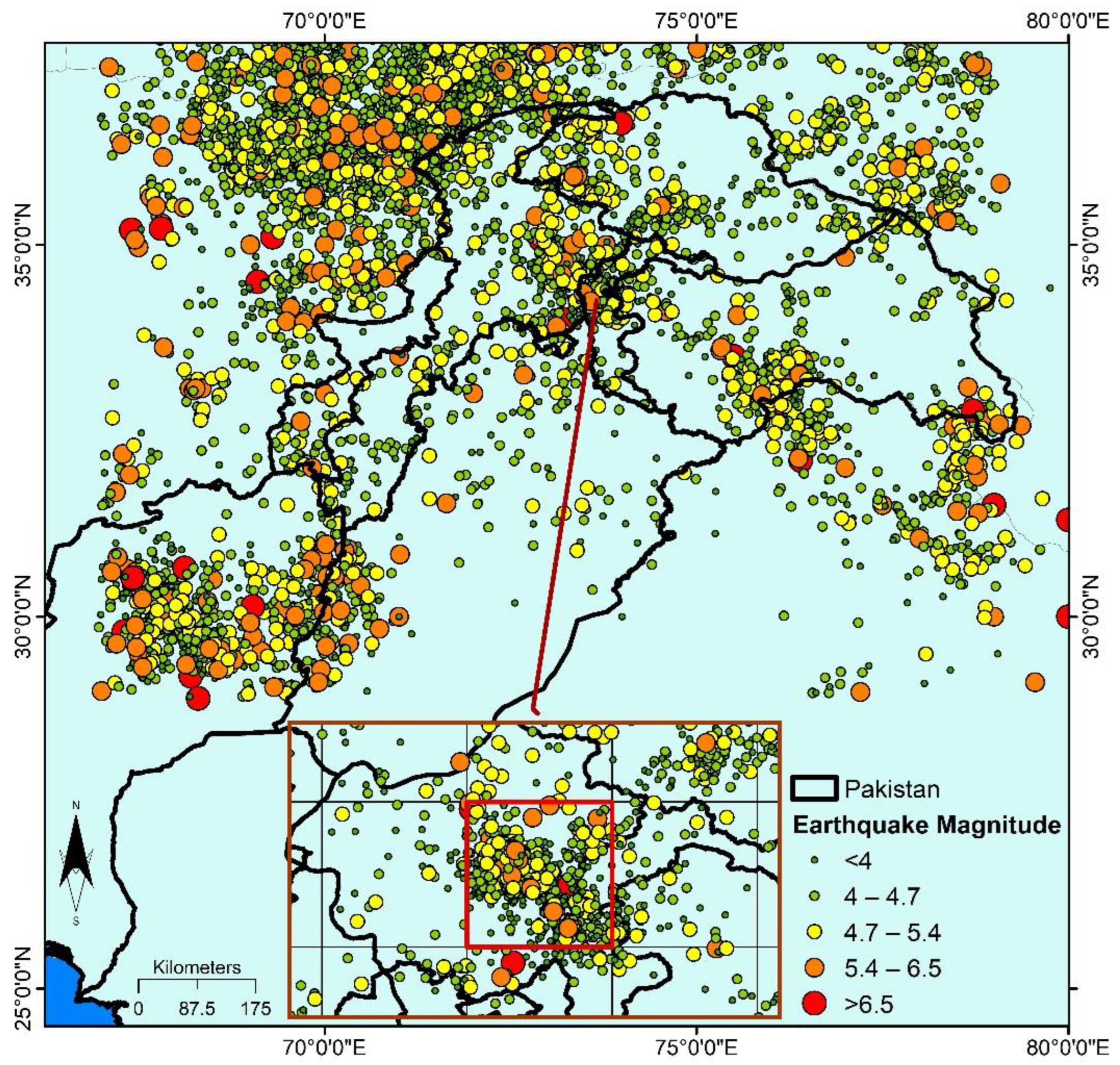
Earthquake is among the major catastrophes that cause significant casualties and damage to infrastructures [9,32,97]. Hindu Kush, Himalayas, and the Karakoram Mountains range in the North of Pakistan are amongst the most seismically lively regions globally. Unfortunately, the North of Pakistan has a record of suffering mild to rigorous and, at times, overwhelming earthquakes, primarily due to its presence at the boundary of the Indian and Eurasian plates [27,35]. Although naturally occurring earthquakes cannot be stopped, their prediction and adequate protection measures can prevent the loss of human life and several valuables.

A mechanism suitable for earthquake prediction that can offer positive predictions is a pressing need at present. A system that is competent in earthquake prediction should predict the accurate location, exact magnitude range, a specific incidence timespan, and the likelihood of incidence. However, no such comprehensive earthquake prediction system has existed to date [8,27]. Several researchers have tackled this problem individually, and investigations have been conducted to predict some of the aforementioned characteristics. However, a holistic study is missing.

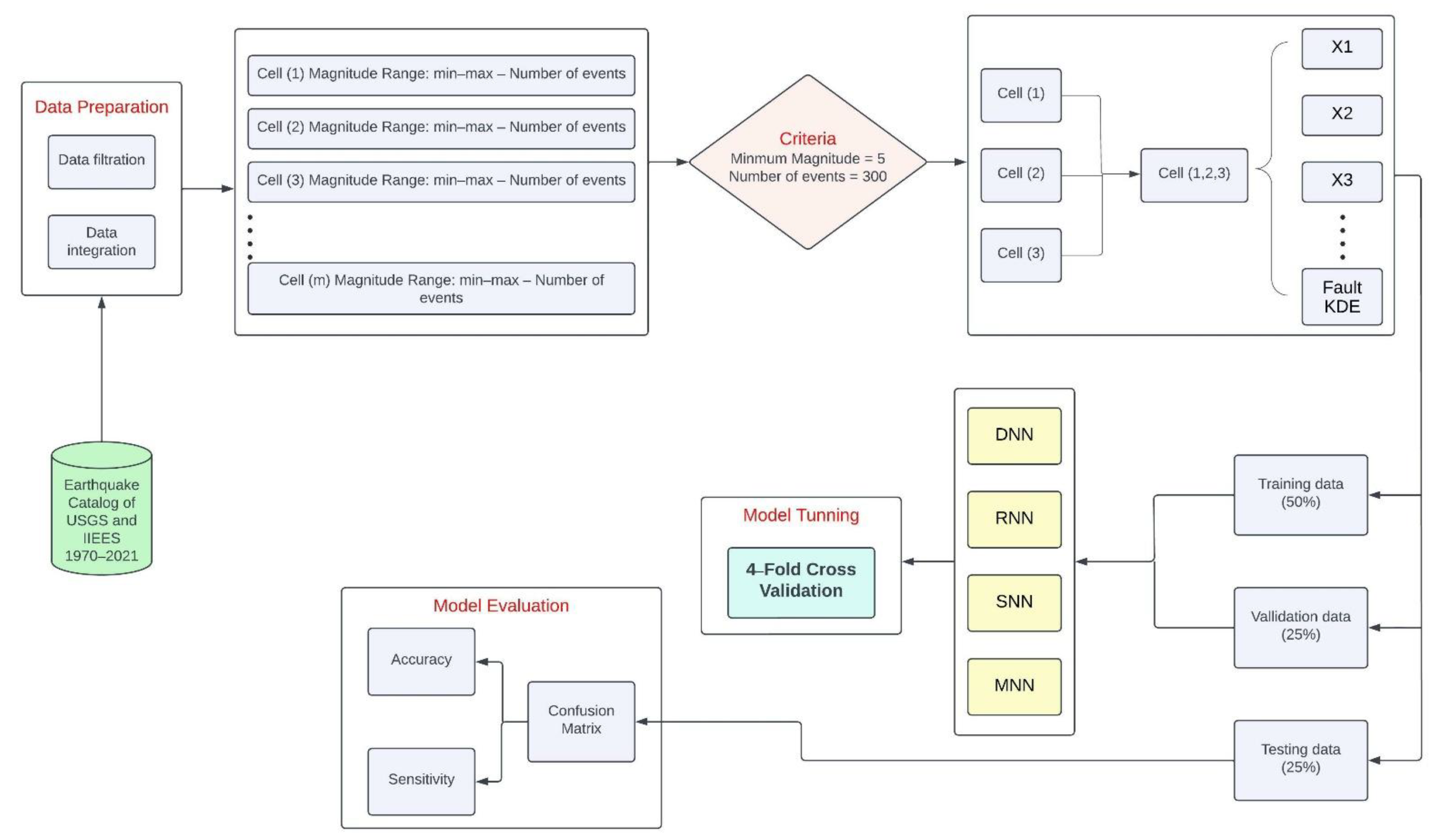
The present study attempts to predict earthquakes of Richter magnitude greater than or equal to 3 in Northern Pakistan using four models (two ML and two DL models): DNN, RNN, SNN, and MNN, combined with 20 seismicity indicators from previously conducted investigations. The arithmetically computed seismicity indicators from the former earthquakes signify the seismic trend of the region. These indicators were used as input to the approaches for earthquake prediction. The seismic indicators were mathematically computed using the records from the earthquake catalog of IIEES and USGS.

Interestingly, some former investigations [8,10] suggested that the cutoff magnitude centered on the GR law must be computed in advance. Moreover, following the calculation of the cutoff magnitude, all events below the computed cutoff magnitude must be excluded. The reason for doing this is to safeguard that inadequate and deceptive information is not fed into the model [10]. Nevertheless, this approach of computing and utilizing the cutoff magnitude results in dropping a big chunk of the data, which is not suitable for operating the models. Therefore, the present research did not apply the cutoff magnitude to the data but excluded all the events with a Richter Mw less than 3.

The seismic variables used in this study are listed in Table 3. These include 16 traditionally used variables and the variables of longitude, latitude, and depth, and a new variable FD. The variables of depth and FD were identified by IGA as being spatial variables of intermediate significance. Therefore, to further investigate the role of the FD variable along with depth, the four used algorithms were operated with distinct sequences of input variables presented in Table 5.

It is important to point out that the variables (X1, X2, X3, X4, and X5) with low IGA values were not removed from the input vector, which is the opposite of the widespread practice of excluding such variables. The reasoning for not excluding these variables stems from the notion that a variable’s effectiveness correspondingly hinges on the capability of the fundamental model. A practical model would benefit from the valuable information coming from less important variables and could offer improved predictions. It is also important to mention that several architectures with distinct hyperparameters were tested to locate the perfect DNN model. The model with the most excellent validation accuracy was chosen as the ideal model. The details of the perfect structure of the DNN model for variable set 3 are listed in Table 7.

Contemplating the two variables of depth and FD, it appears that MNN and SNN were able to utilize the underlying information held by these variables. However, the DNN and RNN could not successfully exploit these two variables. Meanwhile, MNN was the most successful ML algorithm in terms of utilizing the data stored by the depth and FD variables. The deep neural structure of MNN could be a reason for such efficacy by MNN. Furthermore, this structure can obtain valuable information from minimally associated independent input variables.

To analyze the performance of the used ML and DL models in this study, the accuracy and the sensitivity measures were computed. Accuracy was selected as a generic metric for examining the general implementation of the models. The purpose of using sensitivity was to understand how each model performed for each of the four classes. More specifically, the overall performance of the used models is represented by accuracy, whereas the ability of the models to accurately perceive the earthquakes that occurred is indicated by sensitivity.

Sensitivity values for classes 1 and 4 are higher than those for classes 2 and 3. According to Table 10, the highest sensitivity values for classes 1 and 4 occurred when the models were using variables set 1. The most straightforward explanation for this is that the magnitudes for these classes are more closely linked to the FD variable. The low sensitivity values for classes 2 and 3 relatives to classes 1 and 4 for all models are most likely due to significant noise in the magnitude data.

Even though MNN performs much better than the other considered models in terms of accuracy, the sensitivity values were not the highest for MNN, as can be seen from Table 8, Table 9 and Table 10. The best models in terms of sensitivity for predicting classes 1, 2, 3, and 4 were SNN on the variables set 1, DNN on the variables set 1, RNN on the variables set 2, and MNN on the variables set 1. A closer look at the listed sensitivity results in Table 10 reveals that optimal predictions of classes 1, 3, and 4 occurred when the models were exploiting the additional FD variable. This specifies the appropriateness and practicality of the variable, specifically for predicting large-magnitude earthquakes. Classes 3 and 4 can be predicted with the probability of good sensitivity values using the FD variables.

Moreover, the accuracy for both training and testing data for SNN and MNN, which are ML techniques, is surprisingly more than the DL techniques of DNN and RNN, as can be witnessed from Table 8 and Table 9. Technically, this is impossible because ML employs fewer layers for analysis, whereas DL uses more layers, which leads to more accurate results [86,98]. The constructed ML models demonstrated a markedly higher prediction capability than the DL models. This may mean that the DL models considered the classification problem to be linear while it was nonlinear in its nature. Additionally, the different hyperparameter settings affect the performance of ML and DL models [99]. Even though the hyperparameters were changed, and optimal models were constructed during the training process, the choice of the hyperparameters used for the models might not be compatible with the data considered for the analysis.

The DNN model outperformed other models regarding the sensitivity values for class 1. In some cases, such as for class 2, other models outperformed DNN. Amongst the used models, DNN had the most extraordinary complexity. Therefore, in certain situations, this lower sensitivity might be due to its greater parametrization, as was previously observed in an investigation conducted by Mignan and Broccardo [75]. The authors suggested that, due to the structured and tabular nature of catalog data and the insufficient number of calculated features, NN models with shallow structures might compete with DNNs in earthquake prediction. A few other investigations also observed such an adherence regarding the predictive ability of SNNs and deep learning [100,101]. However, the involvement of several hidden layers in DNN allows for one to understand features at distinct levels of perception [98]. This was a key reason for the better performance of the DNN model as compared to other models.

After learning the superiority of the four models, the prediction abilities of the models per class were assessed. The outcomes demonstrated that when the objective was to utilize a general model to predict both high- and low-magnitude earthquakes, RNN or SNN could be a better choice. Nevertheless, as per the sensitivity analysis of classes 1 and 3, MNN or DNN can be a suitable option, as they can better detect and sense low- and moderate-magnitude earthquakes than other models. Regardless of the size of the network and the substantial number of parameters required for the training of the DNN model, the outcomes showed that this complicated model was considerably effective in employing the information from the FD and depth variables. Additionally, the SNN model outperformed other models in predicting high-magnitude earthquakes. This performance of SNN was unexpected, as its structure is comparatively straightforward, and the associations between the input variables and the higher-magnitude earthquakes are quite complicated.

From the viewpoint of a disaster management organization, any model attempting to predict earthquakes should not produce false alarms, as they can cause massive panic and economic loss [46]. Centered on this notion, specificity, NPV, and PPV were computed for all four classes of the DNN model, and the results are shown in Table 11. The specificity, PPV, and NPV values for class 1 are relatively higher than those in other classes. For class 4, the PPV value of 84.10% for the DNN model is very promising.

The advantages of the proposed methods for earthquake magnitude prediction become clear after a comparison with similar studies published previously in the same region and other parts of the world. Asim, Martínez-Álvarez, Basit and Iqbal [46] utilized four ML techniques, RNN, PRNN, LPBoost Ensemble, and Random Forest, to predict earthquakes in the Hindukush region of Northern Pakistan using eight seismic indicators. These indicators were centered on the eminent geophysical facts of GR’s inverse law, dissemination of distinctive earthquake magnitudes and seismic quiescence, and mathematically computed from the earthquake catalog of the region. The authors observed that the LPBoost Ensemble (79%) and PRNN (79%) have the highest accuracy for validation data, while the LPBoost Ensemble (65%) and RNN (64%) have the highest accuracy for the testing data. Compared to this previously conducted study, the present study used more seismic variables, and the accuracy of most of the models for validation and testing data was relatively higher. For example, the testing accuracy of SNN for variable set 2 was 89.30%, while the testing accuracy of MNN for variable set 1 was 84.9%. Moreover, the DNN model also outperforms all the used models in the previous study in terms of specificity.

Moreover, Aslam, Zafar, Khalil and Azam [34] used eight seismic features based on seismological notions, such as the dissemination of typical earthquake extents, the eminent geophysical specifics of Gutenberg–Richter’s inverse law, and seismic quiescence for earthquake prediction in Northern Pakistan. The authors developed a hybrid classification system based on a Support Vector Regressor (SVR) and Hybrid Neural Network (HNN) for earthquakes greater than or equal to 5.5. The accuracy assessment of the SVR-HNN model revealed that the model has a specificity of 86% and a sensitivity of 61%. However, the model attained an accuracy of 79% for the testing data. Compared to the results of the present study, this previously conducted study not only used fewer variables but also attained relatively less accuracy for the developed model compared to the sensitivity results of most of the models of the present study.

Furthermore, Yousefzadeh, Hosseini and Farnaghi [62] introduced and investigated the impact of spatial parameters on the performance of four ML models, specifically, SNN, DNN, DT, and SVM, for predicting future earthquakes’ magnitude in Iran. The results showed that the SVM and DT model achieved the highest accuracy for training data while DT and DNN achieved the highest accuracy for testing data. The authors also used different variable sets for different models and found that DNN and SVM models better detect intermediate- and high-magnitude earthquakes than other models. As the present study introduced different models than the mentioned study, the outcomes of this study also concluded that the DNN model is better than the other practiced models. This establishes the superiority of DNN compared to other conventional techniques.

Based on the outcomes of the present study, it can be stated that the adopted methods can be assessed for their accuracy in other locations by considering spatial variables. Then, a comparison can be carried out to highlight the limitations or adequacies of the methods for the two cases.

6. Conclusions

In the present study, two ML algorithms of SNN, MNN, and two DL algorithms of RNN, and DNN, were utilized to predict short-term earthquakes in the Northern Part of Pakistan, a seismically active region. An additional seismic variable named FD was used, along with the most frequently utilized seismic variables defined in the earlier research. Three different variable sets containing different variables were separately utilized to check the performance of the individual model in response to different variables. When used in different variable sets, the variables of depth and FD facilitated the accuracy of the used ML and DL earthquake prediction models to a certain extent.

The outcomes demonstrated adequate performances of DNN and SNN in predicting the low-magnitude earthquakes, respectively. The DNN model demonstrated an accuracy of 98% for variables set 2 and class 1, whereas the accuracy was 94% for variables set 1. The SNN model showed an accuracy of 95% for variables set 1 and class 1. However, the performance of both RNN and SNN was more encouraging in dealing with high-magnitude events. The SNN model exhibited an accuracy of 95.80% for variables set 2 and class 4, while the RNN model demonstrated an accuracy of 88.30% for variables set 1 and class 4.

6.1. Limitations

The present study only used historical earthquake records from two open-access sources. For future studies, it is important to acquire data from multiple sources to better represent the documented earthquake events in the area. Moreover, it could also be beneficial to acquire some field data from the relevant authorities in the area. Furthermore, different input variables can also be used along with the variables used in this study to check for their influence on the model performance.

6.2. Implications and Future Research

The model presented in this study can be used to predict earthquakes with low and high magnitudes, as advocated by the accuracy assessment results. Moreover, earthquake prediction systems can be a great deal of help for the concerned authorities. An alert triggered by such a system can allow for controls to activate supplies and halt critical damage-causing systems such as electricity and nuclear power plants to avoid fatalities.

Future research can assess the usability of further DNN architectures, such as CNNs, for earthquake prediction and contrast their functioning with other techniques to establish the most superior model. Additionally, the effect of the FD variable on the performance of other contemporary and conventional methods can also be assessed in the context of other seismic regions.

References

1. Chen, H.; Li, S. Collinear Nonlinear Mixed-Frequency Ultrasound with FEM and Experimental Method for Structural Health Prognosis. Processes 2022, 10, 656. [Google Scholar] [CrossRef]
2. Chen, H.; Liu, M.; Chen, Y.; Li, S.; Miao, Y. Nonlinear Lamb Wave for Structural Incipient Defect Detection with Sequential Probabilistic Ratio Test. Secur. Commun. Netw. 2022, 2022, 9851533. [Google Scholar] [CrossRef]
3. Alam, Z.; Sun, L.; Zhang, C.; Samali, B. Influence of seismic orientation on the statistical distribution of nonlinear seismic response of the stiffness-eccentric structure. Structures 2022, 39, 387–404. [Google Scholar] [CrossRef]
4. Zhang, W.; Liu, X.; Huang, Y.; Tong, M.-N. Reliability-based analysis of the flexural strength of concrete beams reinforced with hybrid BFRP and steel rebars. Archiv. Civ. Mech. Eng. 2022, 22, 171. [Google Scholar] [CrossRef]
5. Zhong, T.; Cheng, M.; Lu, S.; Dong, X.; Li, Y. RCEN: A Deep-Learning-Based Background Noise Suppression Method for DAS-VSP Records. IEEE Geosci. Remote Sens. Lett. 2022, 19, 1–5. [Google Scholar] [CrossRef]
6. Zhu, Z.; Zhu, Z.; Wu, Y.; Han, J. A Prediction Method of Coal Burst Based on Analytic Hierarchy Process and Fuzzy Comprehensive Evaluation. Frontiers in earth science (Lausanne). Front. Earth Sci. 2022, 9, 1424. [Google Scholar] [CrossRef]
7. Liu, E.; Chen, S.; Yan, D.; Deng, Y.; Wang, H.; Jing, Z.; Pan, S. Detrital zircon geochronology and heavy mineral composition constraints on provenance evolution in the western Pearl River Mouth basin, northern south China sea: A source to sink approach. Mar. Pet. Geol. 2022, 145, 105884. [Google Scholar] [CrossRef]
8. Zhu, Z.; Wu, Y.; Liang, Z. Mining-Induced Stress and Ground Pressure Behavior Characteristics in Mining a Thick Coal Seam With Hard Roofs. Front. Earth Sci. 2022, 10, 843191. [Google Scholar] [CrossRef]
9. Guo, Y.; Yang, Y.; Kong, Z.; He, J.; Wu, H. Development of Similar Materials for Liquid-Solid Coupling and Its Application in Water Outburst and Mud Outburst Model Test of Deep Tunnel. Geofluids 2022, 2022, 8784398. [Google Scholar] [CrossRef]
10. Zhang, X.; Ma, F.; Yin, S.; Wallace, C.D.; Soltanian, M.R.; Dai, Z.; Ritzi, R.W.; Ma, Z.; Zhan, C.; Lü, X. Application of upscaling methods for fluid flow and mass transport in multi-scale heterogeneous media: A critical review. Appl. Energy 2021, 303, 117603. [Google Scholar] [CrossRef]
11. Huang, S.; Liu, C. A computational framework for fluid–structure interaction with applications on stability evaluation of breakwater under combined tsunami–earthquake activity. Comput.-Aided Civ. Infrastruct. Eng. 2022, 23. [Google Scholar] [CrossRef]
12. Huang, S.; Huang, M.; Lyu, Y. Seismic performance analysis of a wind turbine with a monopile foundation affected by sea ice based on a simple numerical method. Eng. Appl. Comput. Fluid Mech. 2021, 15, 1113–1133. [Google Scholar] [CrossRef]
13. Li, J.; Cheng, F.; Lin, G.; Wu, C. Improved Hybrid Method for the Generation of Ground Motions Compatible with the Multi-Damping Design Spectra. J. Earthq. Eng. 2022, 1–27. [Google Scholar] [CrossRef]
14. Huang, S.; Lyu, Y.; Sha, H.; Xiu, L. Seismic performance assessment of unsaturated soil slope in different groundwater levels. Landslides 2021, 18, 2813–2833. [Google Scholar] [CrossRef]
15. Guo, L.; Ye, C.; Ding, Y.; Wang, P. Allocation of Centrally Switched Fault Current Limiters Enabled by 5G in Transmission System. IEEE Trans. Power Deliv. 2021, 36, 3231–3241. [Google Scholar] [CrossRef]
16. Guo, C.; Ye, C.; Ding, Y.; Wang, P. A Multi-State Model for Transmission System Resilience Enhancement against Short-Circuit Faults Caused by Extreme Weather Events. IEEE Trans. Power Deliv. 2021, 36, 2374–2385. [Google Scholar] [CrossRef]
17. Teng, H.; Ng, H.D.; Li, K.; Luo, C.; Jiang, Z. Evolution of cellular structures on oblique detonation surfaces. Combust. Flame 2015, 162, 470–477. [Google Scholar] [CrossRef] [Green Version]
18. Sun, W.; Lv, X.; Qiu, M. Distributed Estimation for Stochastic Hamiltonian Systems With Fading Wireless Channels. IEEE Trans. Cybern. 2022, 52, 4897–4906. [Google Scholar] [CrossRef]
19. Gu, M.; Mo, H.; Qiu, J.; Yuan, J.; Xia, Q. Behavior of Floating Stone Columns Reinforced with Geogrid Encasement in Model Tests. Front. Mater. 2022, 9, 980851. [Google Scholar] [CrossRef]
20. Cheng, Y.; Fu, L. Nonlinear seismic inversion by physics-informed Caianiello convolutional neural networks for overpressure prediction of source rocks in the offshore Xihu depression, East China. J. Pet. Sci. Eng. 2022, 215, 110654. [Google Scholar] [CrossRef]
21. Asim, K.M.; Idris, A.; Iqbal, T.; Martínez-Álvarez, F. Seismic indicators based earthquake predictor system using Genetic Programming and AdaBoost classification. Soil Dyn. Earthq. Eng. 2018, 111, 1–7. [Google Scholar] [CrossRef]
22. Paola, J.D.; Schowengerdt, R.A. A detailed comparison of backpropagation neural network and maximum-likelihood classifiers for urban land use classification. IEEE Trans. Geosci. Remote Sens. 1995, 33, 981–996. [Google Scholar] [CrossRef]
23. Reyes, J.; Morales-Esteban, A.; Martínez-Álvarez, F. Neural networks to predict earthquakes in Chile. Appl. Soft Comput. 2013, 13, 1314–1328. [Google Scholar] [CrossRef]
24. Asim, K.M.; Awais, M.; Martínez–Álvarez, F.; Iqbal, T. Seismic activity prediction using computational intelligence techniques in northern Pakistan. Acta Geophys. 2017, 65, 919–930. [Google Scholar] [CrossRef]
25. Rasel, R.I.; Sultana, N.; Islam, G.A.; Islam, M.; Meesad, P. Spatio-temporal seismic data analysis for predicting earthquake: Bangladesh perspective. In Proceedings of the 2019 Research, Invention, and Innovation Congress (RI2C), Bangkok, Thailand, 11–13 December 2019; pp. 1–5. [Google Scholar]
26. Ullah, I.; Aslam, B.; Shah, S.H.I.A.; Tariq, A.; Qin, S.; Majeed, M.; Havenith, H.-B. An Integrated Approach of Machine Learning, Remote Sensing, and GIS Data for the Landslide Susceptibility Mapping. Land 2022, 11, 1265. [Google Scholar] [CrossRef]
27. Khalil, U.; Imtiaz, I.; Aslam, B.; Ullah, I.; Tariq, A.; Qin, S. Comparative analysis of machine learning and multi-criteria decision making techniques for landslide susceptibility mapping of Muzaffarabad district. Front. Environ. Sci. 2022, 10, 1–19. [Google Scholar] [CrossRef]
28. Sharifi, A.; Mahdipour, H.; Moradi, E.; Tariq, A. Agricultural Field Extraction with Deep Learning Algorithm and Satellite Imagery. J. Indian Soc. Remote Sens. 2022, 50, 417–423. [Google Scholar] [CrossRef]
29. Bera, D.; Das Chatterjee, N.; Mumtaz, F.; Dinda, S.; Ghosh, S.; Zhao, N.; Bera, S.; Tariq, A. Integrated Influencing Mechanism of Potential Drivers on Seasonal Variability of LST in Kolkata Municipal Corporation, India. Land 2022, 11, 1461. [Google Scholar] [CrossRef]
30. Fu, C.; Cheng, L.; Qin, S.; Tariq, A.; Liu, P.; Zou, K.; Chang, L. Timely Plastic-Mulched Cropland Extraction Method from Complex Mixed Surfaces in Arid Regions. Remote Sens. 2022, 14, 4051. [Google Scholar] [CrossRef]
31. Majeed, M.; Lu, L.; Haq, S.M.; Waheed, M.; Sahito, H.A.; Fatima, S.; Aziz, R.; Bussmann, R.W.; Tariq, A.; Ullah, I.; et al. Spatiotemporal Distribution Patterns of Climbers along an Abiotic Gradient in Jhelum District, Punjab, Pakistan. Forests 2022, 13, 1244. [Google Scholar] [CrossRef]
32. Tariq, A.; Yan, J.; Gagnon, A.S.; Riaz Khan, M.; Mumtaz, F. Mapping of cropland, cropping patterns and crop types by combining optical remote sensing images with decision tree classifier and random forest. Geo-Spat. Inf. Sci. 2022, 1–19. [Google Scholar] [CrossRef]
33. Morales-Esteban, A.; Martínez-Álvarez, F.; Troncoso, A.; Justo, J.; Rubio-Escudero, C. Pattern recognition to forecast seismic time series. Expert Syst. Appl. 2010, 37, 8333–8342. [Google Scholar] [CrossRef]
34. Martínez-Álvarez, F.; Reyes, J.; Morales-Esteban, A.; Rubio-Escudero, C. Determining the best set of seismicity indicators to predict earthquakes. Two case studies: Chile and the Iberian Peninsula. Knowl.-Based Syst. 2013, 50, 198–210. [Google Scholar] [CrossRef]
35. Last, M.; Rabinowitz, N.; Leonard, G. Predicting the maximum earthquake magnitude from seismic data in Israel and its neighboring countries. PLoS ONE 2016, 11, e0146101. [Google Scholar] [CrossRef] [Green Version]
36. Asim, K.M.; Idris, A.; Iqbal, T.; Martínez-Álvarez, F. Earthquake prediction model using support vector regressor and hybrid neural networks. PLoS ONE 2018, 13, e0199004. [Google Scholar] [CrossRef] [Green Version]
37. Mahmoudi, J.; Arjomand, M.A.; Rezaei, M.; Mohammadi, M.H. Predicting the earthquake magnitude using the multilayer perceptron neural network with two hidden layers. Civ. Eng. J. 2016, 2, 1–12. [Google Scholar] [CrossRef]
38. Lin, J.-W.; Chao, C.-T.; Chiou, J.-S. Determining neuronal number in each hidden layer using earthquake catalogues as training data in training an embedded back propagation neural network for predicting earthquake magnitude. IEEE Access 2018, 6, 52582–52597. [Google Scholar] [CrossRef]
39. Kislov, K.; Gravirov, V. Deep artificial neural networks as a tool for the analysis of seismic data. Seism. Instrum. 2018, 54, 8–16. [Google Scholar] [CrossRef]
40. Florido, E.; Aznarte, J.L.; Morales-Esteban, A.; Martínez-Álvarez, F. Earthquake magnitude prediction based on artificial neural networks: A survey. Croat. Oper. Res. Rev. 2016, 7, 159–169. [Google Scholar]
41. Panakkat, A.; Adeli, H. Recurrent neural network for approximate earthquake time and location prediction using multiple seismicity indicators. Comput.-Aided Civ. Infrastruct. Eng. 2009, 24, 280–292. [Google Scholar] [CrossRef]
42. Asim, K.; Martínez-Álvarez, F.; Basit, A.; Iqbal, T. Earthquake magnitude prediction in Hindukush region using machine learning techniques. Nat. Hazards 2017, 85, 471–486. [Google Scholar] [CrossRef]
43. Li, S.; Yang, S.; Wang, Y.; Yue, W.; Qiao, J. A modular neural network-based population prediction strategy for evolutionary dynamic multi-objective optimization. Swarm Evol. Comput. 2021, 62, 100829. [Google Scholar] [CrossRef]
44. Le, X.-H.; Ho, H.V.; Lee, G.; Jung, S. Application of long short-term memory (LSTM) neural network for flood forecasting. Water 2019, 11, 1387. [Google Scholar]
45. Sarwinda, D.; Paradisa, R.H.; Bustamam, A.; Anggia, P. Deep learning in image classification using residual network (ResNet) variants for detection of colorectal cancer. Procedia Comput. Sci. 2021, 179, 423–431. [Google Scholar] [CrossRef]
46. Jalayer, S.; Sharifi, A.; Abbasi-Moghadam, D.; Tariq, A.; Qin, S. Modeling and Predicting Land Use Land Cover Spatiotemporal Changes: A Case Study in Chalus Watershed, Iran. IEEE J. Sel. Top. Appl. Earth Obs. Remote Sens. 2022, 15, 5496–5513. [Google Scholar] [CrossRef]
47. Sadiq Fareed, M.M.; Raza, A.; Zhao, N.; Tariq, A.; Younas, F.; Ahmed, G.; Ullah, S.; Jillani, S.F.; Abbas, I.; Aslam, M. Predicting Divorce Prospect Using Ensemble Learning: Support Vector Machine, Linear Model, and Neural Network. Comput. Intell. Neurosci. 2022, 2022, 3687598. [Google Scholar] [CrossRef]
48. Ghaderizadeh, S.; Abbasi-Moghadam, D.; Sharifi, A.; Tariq, A.; Qin, S. Multiscale Dual-Branch Residual Spectral-Spatial Network With Attention for Hyperspectral Image Classification. IEEE J. Sel. Top. Appl. Earth Obs. Remote Sens. 2022, 15, 5455–5467. [Google Scholar] [CrossRef]
49. Wahla, S.S.; Kazmi, J.H.; Sharifi, A.; Shirazi, S.A.; Tariq, A.; Joyell Smith, H. Assessing spatio-temporal mapping and monitoring of climatic variability using SPEI and RF machine learning models. Geocarto Int. 2022, 1–20. [Google Scholar] [CrossRef]
50. Tariq, A.; Mumtaz, F.; Zeng, X.; Baloch, M.Y.J.; Moazzam, M.F.U. Spatio-temporal variation of seasonal heat islands mapping of Pakistan during 2000–2019, using day-time and night-time land surface temperatures MODIS and meteorological stations data. Remote Sens. Appl. Soc. Environ. 2022, 27, 100779. [Google Scholar] [CrossRef]
51. Tariq, A.; Siddiqui, S.; Sharifi, A.; Hassan, S.; Ahmad, I. Impact of spatio-temporal land surface temperature on cropping pattern and land use and land cover changes using satellite imagery, Hafizabad District, Punjab, Province of Pakistan. Arab. J. Geosci. 2022, 15, 1–16. [Google Scholar] [CrossRef]
52. Tariq, A.; Shu, H. CA-Markov chain analysis of seasonal land surface temperature and land use landcover change using optical multi-temporal satellite data of Faisalabad, Pakistan. Remote Sens. 2020, 12, 3402. [Google Scholar] [CrossRef]
53. Abbas, I.; Liu, J.; Amin, M.; Tariq, A.; Tunio, M.H. Strawberry fungal leaf scorch disease identification in real-time strawberry field using deep learning architectures. Plants 2021, 10, 2643. [Google Scholar] [CrossRef] [PubMed]
54. Melin, P.; Miramontes, I.; Prado-Arechiga, G. A hybrid model based on modular neural networks and fuzzy systems for classification of blood pressure and hypertension risk diagnosis. Expert Syst. Appl. 2018, 107, 146–164. [Google Scholar] [CrossRef]
55. Aslam, B.; Maqsoom, A.; Tahir, M.D.; Ullah, F.; Rehman, M.S.U.; Albattah, M. Identifying and Ranking Landfill Sites for Municipal Solid Waste Management: An Integrated Remote Sensing and GIS Approach. Buildings 2022, 12, 605. [Google Scholar] [CrossRef]
56. Munawar, H.S.; Ullah, F.; Qayyum, S.; Khan, S.I.; Mojtahedi, M. UAVs in disaster management: Application of integrated aerial imagery and convolutional neural network for flood detection. Sustainability 2021, 13, 7547. [Google Scholar] [CrossRef]
57. Atif, S.; Umar, M.; Ullah, F. Investigating the flood damages in Lower Indus Basin since 2000: Spatiotemporal analyses of the major flood events. Nat. Hazards 2021, 108, 2357–2383. [Google Scholar] [CrossRef]
58. Aslam, B.; Maqsoom, A.; Khalid, N.; Ullah, F.; Sepasgozar, S. Urban overheating assessment through prediction of surface temperatures: A case study of karachi, Pakistan. ISPRS Int. J. Geo-Inf. 2021, 10, 539. [Google Scholar] [CrossRef]
59. Maqsoom, A.; Aslam, B.; Yousafzai, A.; Ullah, F.; Ullah, S.; Imran, M. Extracting built-up areas from spectro-textural information using machine learning. Soft Comput. 2022, 26, 7789–7808. [Google Scholar] [CrossRef]
60. Tariq, A.; Shu, H.; Gagnon, A.S.; Li, Q.; Mumtaz, F.; Hysa, A.; Siddique, M.A.; Munir, I. Assessing Burned Areas in Wildfires and Prescribed Fires with Spectral Indices and SAR Images in the Margalla Hills of Pakistan. Forests 2021, 12, 1371. [Google Scholar] [CrossRef]
61. Ahmad, A.; Ahmad, S.R.; Gilani, H.; Tariq, A.; Zhao, N.; Aslam, R.W.; Mumtaz, F. A Synthesis of Spatial Forest Assessment Studies Using Remote Sensing Data and Techniques in Pakistan. Forests 2021, 12, 1211. [Google Scholar] [CrossRef]
62. Hu, P.; Sharifi, A.; Tahir, M.N.; Tariq, A.; Zhang, L.; Mumtaz, F.; Shah, S.H.I.A. Evaluation of Vegetation Indices and Phenological Metrics Using Time-Series MODIS Data for Monitoring Vegetation Change in Punjab, Pakistan. Water 2021, 13, 2550. [Google Scholar] [CrossRef]
63. Tariq, A.; Shu, H.; Kuriqi, A.; Siddiqui, S.; Gagnon, A.S.; Lu, L.; Linh, N.T.T.; Pham, Q.B. Characterization of the 2014 Indus River Flood Using Hydraulic Simulations and Satellite Images. Remote Sens. 2021, 13, 2053. [Google Scholar] [CrossRef]
64. Tariq, A.; Riaz, I.; Ahmad, Z. Land surface temperature relation with normalized satellite indices for the estimation of spatio-temporal trends in temperature among various land use land cover classes of an arid Potohar region using Landsat data. Environ. Earth Sci. 2020, 79, 40. [Google Scholar] [CrossRef]
65. Adeli, H.; Panakkat, A. A probabilistic neural network for earthquake magnitude prediction. Neural Netw. 2009, 22, 1018–1024. [Google Scholar] [CrossRef] [PubMed]
66. Morales-Esteban, A.; Martínez-Álvarez, F.; Reyes, J. Earthquake prediction in seismogenic areas of the Iberian Peninsula based on computational intelligence. Tectonophysics 2013, 593, 121–134. [Google Scholar] [CrossRef]
67. Hetényi, G.; Epard, J.-L.; Colavitti, L.; Hirzel, A.H.; Kiss, D.; Petri, B.; Scarponi, M.; Schmalholz, S.M.; Subedi, S. Spatial relation of surface faults and crustal seismicity: A first comparison in the region of Switzerland. Acta Geod. Geophys. 2018, 53, 439–461. [Google Scholar] [CrossRef] [Green Version]
68. Bailey, T.C.; Gatrell, A.C. Interactive Spatial Data Analysis; Longman Scientific & Technical Essex: Harlow Essex, UK, 1995; Volume 413.
69. De Smith, M.J.; Goodchild, M.F.; Longley, P. Geospatial Analysis: A Comprehensive Guide to Principles, Techniques and Software Tools; Troubador Publishing Ltd.: Market Harborough, UK, 2007. [Google Scholar]
70. Hu, Z.; Rao, K.R. Particulate air pollution and chronic ischemic heart disease in the eastern United States: A county level ecological study using satellite aerosol data. Environ. Health 2009, 8, 26. [Google Scholar] [CrossRef] [Green Version]
71. Lopez-Martin, M.; Carro, B.; Sanchez-Esguevillas, A.; Lloret, J. Shallow neural network with kernel approximation for prediction problems in highly demanding data networks. Expert Syst. Appl. 2019, 124, 196–208. [Google Scholar] [CrossRef]
72. Ustebay, S.; Turgut, Z.; Aydin, M.A. Cyber attack detection by using neural network approaches: Shallow neural network, deep neural network and autoencoder. In Proceedings of the International Conference on Computer Networks, New York, NY, USA, 24 February 2019; pp. 144–155. Available online: https://link.springer.com/chapter/10.1007/978-3-030-21952-9_11 (accessed on 12 October 2022).
73. Dufera, T.T. Deep neural network for system of ordinary differential equations: Vectorized algorithm and simulation. Mach. Learn. Appl. 2021, 5, 100058. [Google Scholar] [CrossRef]
74. Bayat, M.; Ghorbanpour, M.; Zare, R.; Jaafari, A.; Pham, B.T. Application of artificial neural networks for predicting tree survival and mortality in the Hyrcanian forest of Iran. Comput. Electron. Agric. 2019, 164, 104929. [Google Scholar] [CrossRef]
75. Wang, X.; Gao, L.; Mao, S. CSI phase fingerprinting for indoor localization with a deep learning approach. IEEE Internet Things J. 2016, 3, 1113–1123. [Google Scholar] [CrossRef]
76. Moghar, A.; Hamiche, M. Stock market prediction using LSTM recurrent neural network. Procedia Comput. Sci. 2020, 170, 1168–1173. [Google Scholar] [CrossRef]
77. Chen, J.; Jing, H.; Chang, Y.; Liu, Q. Gated recurrent unit based recurrent neural network for remaining useful life prediction of nonlinear deterioration process. Reliab. Eng. Syst. Saf. 2019, 185, 372–382. [Google Scholar] [CrossRef]
78. Zhang, Y.; Xiong, R.; He, H.; Pecht, M.G. Long short-term memory recurrent neural network for remaining useful life prediction of lithium-ion batteries. IEEE Trans. Veh. Technol. 2018, 67, 5695–5705. [Google Scholar] [CrossRef]
79. Russell, N.; Bakker, H.; Chaplin, R. Modular neural network modelling for long-range prediction of an evaporator. Control. Eng. Pract. 2000, 8, 49–59. [Google Scholar] [CrossRef]
80. Sánchez, D.; Melin, P.; Castillo, O. Optimization of modular granular neural networks using a hierarchical genetic algorithm based on the database complexity applied to human recognition. Inf. Sci. 2015, 309, 73–101. [Google Scholar] [CrossRef]
81. González, B.; Valdez, F.; Melin, P.; Prado-Arechiga, G. Fuzzy logic in the gravitational search algorithm enhanced using fuzzy logic with dynamic alpha parameter value adaptation for the optimization of modular neural networks in echocardiogram recognition. Appl. Soft Comput. 2015, 37, 245–254. [Google Scholar] [CrossRef]
82. Varela-Santos, S.; Melin, P. A new modular neural network approach with fuzzy response integration for lung disease classification based on multiple objective feature optimization in chest X-ray images. Expert Syst. Appl. 2021, 168, 114361. [Google Scholar] [CrossRef]
83. Zhang, Y.; Xie, Y.; Zhang, Y.; Qiu, J.; Wu, S. The adoption of deep neural network (DNN) to the prediction of soil liquefaction based on shear wave velocity. Bull. Eng. Geol. Environ. 2021, 80, 5053–5060. [Google Scholar] [CrossRef]
84. Adege, A.B.; Lin, H.-P.; Tarekegn, G.B.; Jeng, S.-S. Applying deep neural network (DNN) for robust indoor localization in multi-building environment. Appl. Sci. 2018, 8, 1062. [Google Scholar] [CrossRef] [Green Version]
85. Adege, A.B.; Yen, L.; Lin, H.-p.; Yayeh, Y.; Li, Y.R.; Jeng, S.-S.; Berie, G. Applying Deep Neural Network (DNN) for large-scale indoor localization using feed-forward neural network (FFNN) algorithm. In Proceedings of the 2018 IEEE International Conference on Applied System Invention (ICASI), Tokyo, Japan, 13–17 April 2018; pp. 814–817. [Google Scholar]
86. Van Dao, D.; Jaafari, A.; Bayat, M.; Mafi-Gholami, D.; Qi, C.; Moayedi, H.; Van Phong, T.; Ly, H.-B.; Le, T.-T.; Trinh, P.T. A spatially explicit deep learning neural network model for the prediction of landslide susceptibility. Catena 2020, 188, 104451. [Google Scholar]
87. Zhong, G.; Ling, X.; Wang, L.N. From shallow feature learning to deep learning: Benefits from the width and depth of deep architectures. Wiley Interdiscip. Rev. Data Min. Knowl. Discov. 2019, 9, e1255. [Google Scholar] [CrossRef] [Green Version]
88. Feng, X.; Yang, J.; Lipton, Z.C.; Small, S.A.; Provenzano, F.A.; Initiative, A.S.D.N. Deep learning on MRI affirms the prominence of the hippocampal formation in Alzheimer’s disease classification. bioRxiv 2018, 10, 456277. [Google Scholar]
89. Bosire, A. Recurrent neural network training using ABC algorithm for traffic volume prediction. Informatica 2019, 43. [Google Scholar] [CrossRef]
90. Nikoobakht, S.; Azarafza, M.; Akgün, H.; Derakhshani, R. Landslide Susceptibility Assessment by Using Convolutional Neural Network. Appl. Sci. 2022, 12, 5992. [Google Scholar] [CrossRef]
91. Chung, H.; Shin, K.-S. Genetic algorithm-optimized long short-term memory network for stock market prediction. Sustainability 2018, 10, 3765. [Google Scholar] [CrossRef] [Green Version]
92. Liu, Z.; Sun, X.; Wang, S.; Pan, M.; Zhang, Y.; Ji, Z. Midterm power load forecasting model based on kernel principal component analysis and back propagation neural network with particle swarm optimization. Big Data 2019, 7, 130–138. [Google Scholar] [CrossRef] [Green Version]
93. Krogh, A.; Hertz, J. A simple weight decay can improve generalization. Adv. Neural Inf. Process. Syst. 1991, 4, 23. [Google Scholar]
94. Srivastava, N.; Hinton, G.; Krizhevsky, A.; Sutskever, I.; Salakhutdinov, R. Dropout: A simple way to prevent neural networks from overfitting. J. Mach. Learn. Res. 2014, 15, 1929–1958. [Google Scholar]
95. Garg, Y.; Masih, A.; Sharma, U. Predicting Bridge Damage during Earthquake Using Machine Learning Algorithms. In Proceedings of the 2021 11th International Conference on Cloud Computing, Data Science & Engineering (Confluence), Uttar Pradesh, India, 28–29 January 2021; pp. 725–728. [Google Scholar]
96. Toolan, F.; Carthy, J. Feature selection for spam and phishing detection. In Proceedings of the 2010 eCrime Researchers Summit, Dallas, TX, USA, 10–18 October 2010; pp. 1–12. [Google Scholar]
97. Mitchell, T.M. Advances in Neural Information Processing Systems 4 (NIPS 1991); Learning, M., Ed.; McGraw-Hill: New York, NY, USA, 1997; pp. 154–200. [Google Scholar]
98. Khalil, U.; Aslam, B.; Kazmi, Z.A.; Maqsoom, A.; Qureshi, M.I.; Azam, S.; Nawaz, A. Integrated support vector regressor and hybrid neural network techniques for earthquake prediction along Chaman fault, Baluchistan. Arab. J. Geosci. 2021, 14, 2192. [Google Scholar] [CrossRef]
99. Khalil, U.; Aslam, B.; Maqsoom, A. Afghanistan earthquake 2015 aftershocks analysis for a better understanding of the seismicity behavior for future assessment. Acta Geophys. 2021, 69, 1189–1197. [Google Scholar] [CrossRef]
100. Bevilacqua, V.; Brunetti, A.; Guerriero, A.; Trotta, G.F.; Telegrafo, M.; Moschetta, M. A performance comparison between shallow and deeper neural networks supervised classification of tomosynthesis breast lesions images. Cogn. Syst. Res. 2019, 53, 3–19. [Google Scholar] [CrossRef]
101. Nicolis, O.; Plaza, F.; Salas, R. Prediction of intensity and location of seismic events using deep learning. Spat. Stat. 2021, 42, 100442. [Google Scholar] [CrossRef]
Figure 1. The methodological framework of the study.
Buildings 12 01713 g001
Figure 2. Frequency of earthquake occurrence per year from 1970 until 2021 in Northern Pakistan.
Buildings 12 01713 g002
Figure 3. Distribution of earthquakes based on the magnitude of occurrence (greater than 3 Richter) and location from 1970 until 2021 in Pakistan and its surroundings.
Buildings 12 01713 g003