Article

Cost-Based Optimization of Isolated Footing in Cohesive Soils Using Generalized Reduced Gradient Method

1
NUST Institute of Civil Engineering, National University of Sciences and Technology (NUST), Islamabad 44000, Pakistan
2
Department of Civil Engineering, University of Management and Technology, C-II Johar Town, Lahore 54000, Pakistan
3
Department of Civil and Environmental Engineering, Pusan National University, Busan 46241, Korea
4
College of Engineering and Technology, American University of the Middle East, Egaila 54200, Kuwait
*
Authors to whom correspondence should be addressed.
Buildings 2022, 12(10), 1646; https://doi.org/10.3390/buildings12101646
Submission received: 1 September 2022 / Revised: 29 September 2022 / Accepted: 6 October 2022 / Published: 10 October 2022
(This article belongs to the Special Issue Advances in Soils and Foundations)

Abstract

:
This study presents a cost-based optimization model for the design of isolated foundations in cohesive soils. The optimization algorithm not only incorporates safety requirements in the form of ultimate limit state (ULS) and serviceability limit state (SLS) criteria but also deals with the economics simultaneously. In that regard, the generalized reduced gradient (GRG) method is used for the optimization purpose to achieve the least construction cost of an isolated foundation along with the integration of design parameters as optimization variables. The optimization technique is elaborated using a design example in silty clayey soil and the results of the optimized design are compared with those of the conventional design. The optimization model shows that the optimized design can reduce the construction cost by up to 44% as compared to the conventional design cost for the particular example. Moreover, a sensitivity analysis is also performed to evaluate the quantitative impact of cohesive soil properties, design load, and groundwater table on the construction cost. The results indicate that the construction cost majorly depends on the combined effect of four key parameters: Young’s modulus, recompression index, design load, and groundwater table.

1. Introduction

A shallow foundation design should be safe as well as economical. A design is acceptable when it satisfies arithmetic checks of safety along with economics. The ultimate limit state (ULS) and serviceability limit state (SLS) are regarded as the two computational checks of safety in foundation design [1,2]. In general, while designing a foundation, safety is generally prioritized over the economic aspect of the project. Ideally, various conventional design approaches can be used to justify the safety requirements, i.e., ultimate limit state (ULS) and serviceability limit state (SLS), but the least construction cost governs the final acceptable design. Wellington, the father of engineering economy, defined economy as the key parameter for a successful design project [3]. The importance of engineering economics is well established and is described in various literature works [2,4,5,6]. However, most of the discussion is still at the academic and conceptual level. Additionally, conventional design approaches are based on the trial-and-error method, which requires several iterations to approach an economical and safe foundation design. These kinds of approaches, in the absence of any particular guidelines, are monotonous and time-consuming. Therefore, there is a need for developing a comprehensive foundation design framework that explicitly addresses ULS, SLS, and economics simultaneously leading to a progressive sustainable infrastructure.
The scope of the existing literature regarding the optimization of an isolated footing design is limited to safety requirements. Rawat et al. [7] suggested a cost optimization technique for the design of isolated footing considering the structural aspects of the footing design. However, the geotechnical design of an isolated foundation is imperative and must be considered prior to the structural design. Al-Ansari [8] presented an analytical optimization method to compute the structural cost of the reinforced concrete isolated foundation. Kimmerling [9] worked on the economical and safe design of a shallow foundation for a bridge based on Limit State Design (LSD) and Load and Resistance Factored Design (LRFD) procedures. Stolyarov [10] developed an analytical method to optimize the foundation design by determining the minimum volume of the foundation. According to this study, the minimum volume of foundation could be obtained by simultaneous computations of the base and body of the footing. A minimum volume of concrete cannot be considered as the only factor controlling the cost of the foundation since several other factors govern the foundation construction cost, i.e., execution, formwork, reinforcement, backfill, etc. Bhavikatti et al. [11] proposed a linear optimization technique for optimizing a column footing and reported 8–10% savings in cost. However, this work was based on a linear optimization of reinforcement only and did not consider the other structural and geotechnical design aspects of the isolated foundation. Wang [12] presented a reliability-based method for the cost optimization of foundation design, which was based on the uncertainties related to geotechnical engineering. Chaudhuri et al. [13] developed a constrained binary-coded genetic algorithm for the cost optimization of isolated footing design based on the structural safety requirements using MATLAB. Piegay et al. [14] provided a multiobjective approach for the cost optimization of spread footing using the a Monte Carlo simulation technique. However, the use of the Monte Carlo simulation technique, based on the coefficient of variance values of the soil properties, was not a straightforward solution and design engineers may find it challenging to implement such techniques. Juang et al. [15] presented a new technique called robust geotechnical design (RDG) for the cost optimization of spread footing. Islam et al. [16] formulated a genetic algorithm (GA) to optimize spread footings in sandy soil in which a shallow foundation design process for given soil properties and design loads was framed in an optimization procedure to obtain the least construction cost using the GA technique. Wang et al. [17] proposed the optimization of a foundation design considering the variable parameters controlling the design of a shallow foundation in dry sand. Still, the scope of the research was limited to dry sandy soils only and did not consider the effect of groundwater table on the economics of the construction of the foundation. Jelušič et al. [18] proposed a cost-based mixed integer nonlinear programming (MINLP) optimization technique for the pad footing considering ULS and SLS criteria. In general, all the available cost optimization techniques for isolated footing design are either difficult to implement in most conventional practices or they are based on the structural design approach and target particular structural elements and their performance in various soil types [19,20]. In light of the literature review and to the best of the authors’ knowledge, no design framework has been developed so far that not only considers the cost and safety requirements in cohesive soils simultaneously but also encompasses the quantitative impact of groundwater fluctuation on the construction cost of foundations. Furthermore, the existing frameworks are difficult to implement by design engineers in the field. The current study aims to develop an MS Excel-based design framework using the generalized reduced gradient (GRG) method that explicitly considers cost and safety requirements through a straightforward and user-friendly interface, as MS Excel-based design approaches are quite well-known and well-liked among design engineers.
The generalized reduced gradient is a technique that is used for solving nonlinear problems and the cost-based design of foundation is not a straightforward solution. Therefore, the GRG technique can be employed to solve cost-based design problems. This technique can be utilized through “Excel Solver”, an add-in tool available in excel. The advantage of using this technique over the other conventional techniques is that it is a relatively easy excel-based technique that requires a very short time and few inputs to optimize the design to obtain the least construction cost.
This study presents a novel cost-based optimization technique for the isolated foundation design in cohesive soil using the generalized reduced gradient technique. The fundamental aim of the optimization model is to obtain the minimum construction cost of an isolated footing without any detriment to the safety requirements, i.e., ULS, and SLS criteria. Accordingly, an optimization model was developed based on ULS and SLS design computations followed by cost estimation. Henceforth, a design example is also demonstrated in which the optimization model was applied to an isolated foundation design in cohesive soil (ϕ = 0). Furthermore, a sensitivity analysis was performed to assess the economic impact of cohesive soil properties, groundwater table, and design requirements of the isolated foundation. This study presents a comprehensive cost-effective approach that can be applied to isolated foundation design in cohesive soils without performing several iterations.

2. Basics of Foundation Design in Cohesive Soils and Methods

ULS and SLS are safety criteria for a shallow foundation design. ULS is governed by the required factor of safety (FSr) [1,21] which can be computed through Equation (1).
FS r =   q ult F / BL
where qult (kN/m2) is the ultimate bearing capacity, F (kN) is the applied vertical force in the form of building load, and B (m) and L (m) are the width and length of the foundation, respectively.
There are several theories to evaluate the bearing capacity of a shallow foundation. The models presented by Terzaghi [22], Meyerhof [23], and Vesic [24] are the most commonly used for evaluating the bearing capacity of cohesive soils. For the bearing capacity computation in cohesive soils, the ϕ = 0 condition is considered [4,25,26]. Vesic’s model is more comprehensive and detailed as compared to other bearing capacity models. Therefore, Vesic’s bearing capacity equation [24] was used in this study, as given below
q u = c N c S c d c i c b c + σ z N q s q d q i q b q + 1 2   γ   BN γ s γ d γ i γ b γ
where Sc, Sq, and S γ are shape factors, dc, dq, and d γ are depth factors, i c ,   i q , and i γ are load inclination factors, and b c , ,   b q ,   and   b γ are base inclination factors. In this study, inclination factors were equal to 1 due to the concentric nature of the foundation. Other factors are given below.
S c = 1 + ( B L ) ( N q N c )
S q = 1 + ( B L ) tan ϕ  
S γ = 1 0.4 ( B L )
d c = 1 + 0.4 k
d q = 1 + 2 k   tan ϕ   ( 1 sin ϕ ) 2
d γ = 1
The serviceability limit state (SLS) for a shallow foundation is governed by the allowable settlement of 25 mm [27] which can be evaluated using Equation (9) [4].
δ t =   δ i +   δ c
where δi (mm) is the immediate settlement and δc (mm) is the primary consolidation settlement. δi is given by Equation (10) [28].
δ i = F ( 1 v 2 ) β z E ( BL ) ( 1 2 )
where v is poison’s ratio, E (MPa) is the Young’s modulus, F (kN) is the vertical load, B (m) is the width, L (m) is the length, and βz is the shape factor described in Figure 1 [29], which is approximated by the polynomial function obtained from the relationship of βz vs. L/B and is given by Equation (11).
β z = 0.0017 ( L B ) 2 + 0.0597 ( L B ) + 0.9843
The consolidation settlement can be computed using Equations (12)–(14) [4,30], depending upon the overconsolidation ratio (OCR) and specific conditions as given below,
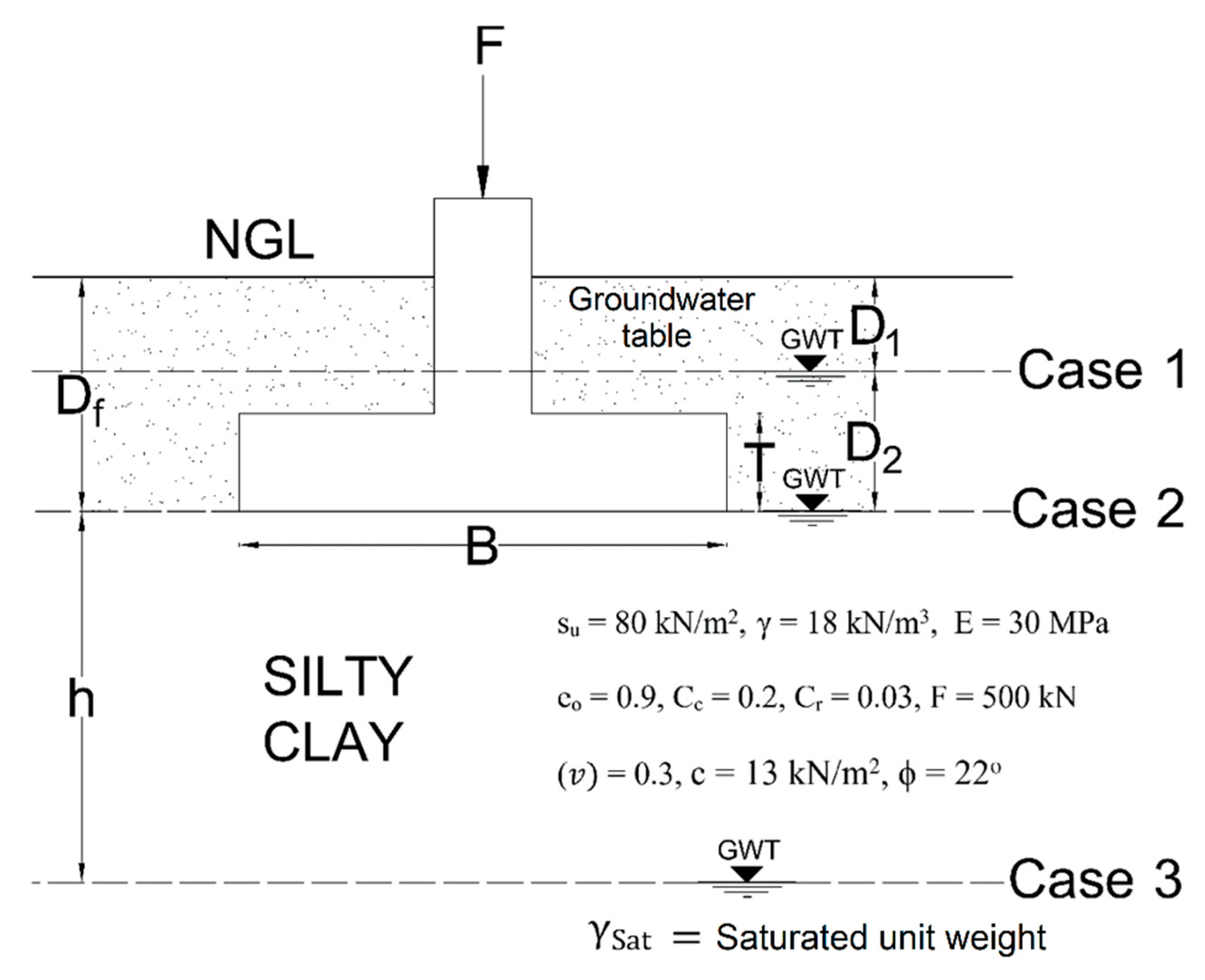
  • Case 1, for normally consolidated soil: (σo = σp)
    δ c = HC c 1 + e o   log ( σ o + Δ σ σ o )
  • Case 2, for overconsolidated soil: (σo+ Δσ < σp)
    δ c = HC r 1 + e o   log ( σ o + Δ σ σ o )
  • Case 3, for overconsolidated soil: (σo < σp < σo+ Δσ)
    δ c = HC r 1 + e o log ( σ p σ o ) + HC c 1 + e o   log ( σ o + Δ σ σ p )
    where σo (kN/m2) is the effective overburden stress, σp (kN/m2) is the preconsolidation pressure, eo is the initial void ratio, H (m) is the clay layer thickness, and Δσ is the stress increase that can be determined with the help of the 2:1 method using Equation (15) [31].
    Δ σ = F ( B + z ) ( L + z )
    where F (kN) is the load, B (m) is the width, L (m) is the length, and z (m) is the depth at H/2 of the clay layer from the base of the footing.

3. Conceptual Framework and Methodology

In general, the design of a shallow foundation is a procedure of specifying the type of foundation and parameters associated with it, i.e., materials and dimensions. The performance of any foundation design is assessed by ULS and SLS criteria. The ULS criterion is given by the factor of safety (FSr), while the SLS criterion is given by the allowable settlement (δr). The ULS criterion is satisfied if the factor of safety after the design process (Equation (1)) comes out to be 3 or more and the SLS criterion is satisfied if the computed settlement lies within the range of 25 mm [17,32].
The cost-effectiveness of a shallow foundation design is an essential part that cannot be ignored. The cost of a project depends on various design parameters which control the construction cost of the foundation. This process of adjusting and minimizing the cost while satisfying the minimum design performance requirements is called the optimization process. The purpose of the optimization of a foundation design is to propose the design parameters that meet ULS and SLS criteria along with the minimum cost. Hence, the design parameters were considered as optimization variables in this study.

3.1. Basics of Generalized Reduced Gradient Method:

In this study, a generalized reduced gradient (GRG) technique was used to optimize a shallow foundation design problem. GRG is considered the most robust and efficient technique for the optimization of nonlinear problems [33,34]. GRG is based on three main parameters, namely, the objective function, decision variables, and constraints. GRG algorithms solve the problems which are nonlinear in nature as the given inequality (16);
Minimize :   g { m + 1 }   ( X ) Subject   to :   g i   ( X ) = 0 ,   i = 1 ,   n eq Constraints :   0   g i ( X   )   u b   ( n + 1 ) ,   i = n eq + 1 ,   m , l b   X i   u b   ( i ) ,   i = 1 ,   n ,
where X is a vector of n decision variables. neq is the number of equality constraints that might be zero, and the gi functions are assumed to be differentiable. lb and ub are the lower bounds and upper bounds of constraints. Then, the nonlinear problem of the form given by inequality (16) is solved by the addition of slack variables, i.e., Xn+1, …, Xn+m. The detailed mathematical programming is beyond the scope of this study and the reader is referred to Lasdon et al. [34].
In this study, an isolated footing in a cohesive soil was designed with the help of the optimization process using the GRG technique in Excel Solver and the optimized design was compared with the conventional design. Excel Solver is an efficient and widely used optimization add-in tool available in MS Excel. It is very efficient to achieve the desired output by varying the assumed parameters in any design. Excel Solver is a kind of what-if analysis that yields the best possible optimal solution for an objective function in a selected target cell of an Excel worksheet. It optimizes the objective function in the target cell by performing iterations on the ranges identified in the user-defined variable value cells that are known as design constraints [35,36]. Excel Solver can be used to optimize the foundation design. The conventional foundation design process begins with an initial trial assuming the design parameters, i.e., width, depth, and length, followed by a revised design if needed. The trial design is checked against SLS and ULS requirements. The final construction cost of the isolated foundation can be set as an objective function in Excel Solver, while width, depth, and length can be treated as adaptable design variables. ULS and SLS requirements in addition to some practical restrictions can be regarded as constraints. Excel Solver optimizes any design problem using linear and nonlinear programming techniques namely generalized reduced gradient (GRG), simplex linear programming (LP), and evolutionary techniques. In this study, the shallow foundation design in cohesive soils was framed in an optimization process using the GRG technique in Excel Solver. The details of the design framework are described in the following sub-sections.

3.1.1. Design Variables

An isolated foundation design is a process of specifying the foundation dimensions which satisfy the safety and economic requirements. These dimensions are treated as design variables. There are three assumed variables of geotechnical foundation design that govern the construction cost of an isolated foundation as given below
  • Embedment depth of foundation (Df)
  • Width of foundation (B)
  • Length of foundation (L)
These design variables can be set as “changing variables” in Excel Solver.

3.1.2. Objective Function

The total construction cost (C) of an isolated footing is taken as the primary objective function, which is a function of the quantities of five activities, namely, excavation (Qe), formwork (Qf), concrete (Qc), reinforcement (Qr), and compacted backfill (Qb) and can be given by Equation (17) [17].
Construction   cos t   ( C ) = Q e R e +   Q f R f +   Q c R c +   Q r R r +   Q b R b
where Re, Rf, Rc, Rc, and Rb are unit rates for excavation, formwork, concrete, reinforcement, and compacted backfill, respectively. In this study, the cost was calculated in the currency of Pakistan, the Pakistani Rupee (PKR). The unit prices were taken from the schedule rates of the National Highway Authority, Pakistan [37]. The unit prices for a shallow foundation construction are summarized in Table 1.
The quantity of excavation (Qe) for the construction of a shallow foundation can be calculated by Equation (18).
Q e = ( B + B o ) ( L + L o ) D f
where B (m), L (m) and Df (m) are the width, length, and depth of foundation, while Lo and Bo are overexcavation distances along the axes of length and width, respectively. It is recommended to use both Bo and Lo values as 0.3 m in foundation design to provide enough space for the installation of the foundation [38]. The quantity of formwork (Qf) can be calculated by Equation (19).
Q f = 2 T   ( B   +   L )
where T is the thickness of footing. The quantity of concrete can be calculated by Equation (20).
Q c =   BLT
The quantity of reinforcement (Qr) of a shallow foundation can be given by Equation (21).
Q r =   kQ c
where k is the coefficient of proportionality that can be taken as 29.67 kg/cm3 [39]. The quantity of backfill (Qb) can be estimated using Equation (22).
Q b =   Q e   Q c

3.1.3. Design Constraints

Design constraints are the upper and lower bound limits of design variables that are used for optimization purpose in any design project. The design is assessed by certain performance requirements namely performance indices (PI) defined in the country codes. The general concept of constraints is illustrated as:
  • PI1 (y1, y2, y3, …, yn) ≥ or ≤ PI1r
  • PI2 (y1, y2, y3, …, yn) ≥ or ≤ PI2r
  •  
  •  
  • PIn (y1, y2, y3, …, yn) ≥ or ≤ PInr.
  • Practical constraints, yil ≤ yi ≤ yiu, I = 1,2, 3, …, n
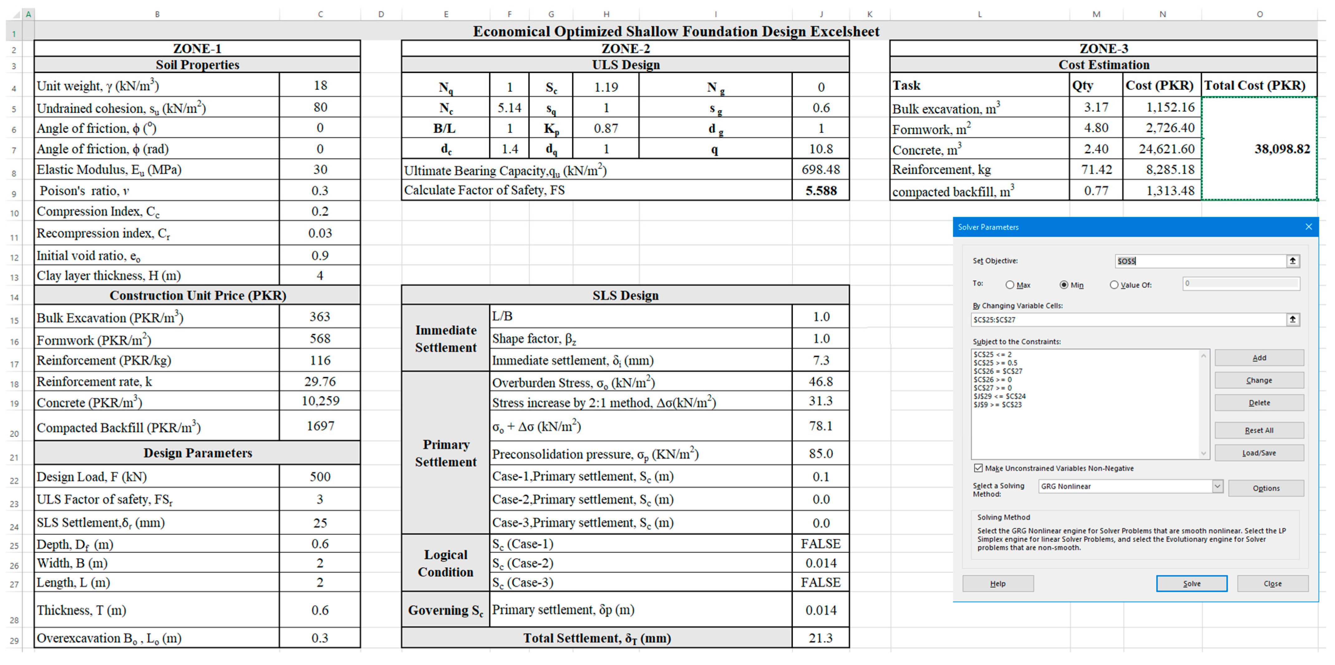
PI is a performance index that must address a certain performance requirement and y1, y2, …, yn are design variables. For example, SLS is one of the performance requirements in a foundation design, which states that settlement should not exceed 25 mm. So, the functional parameters should be adjusted such that the resulting settlement remains within the allowable range. The symbols yil and yiu are lower and upper bound limits. The lower and upper bound limits (yil, yiu) of the design parameters can be understood in a way that the dimensions of the foundation should always be greater than zero. Hence, the lower bound limit (yil) should be greater than zero. Figure 2 shows the procedure of the GRG algorithm for the optimization of the isolated foundation.

4. Design Example

Figure 3 shows an isolated foundation in silty clay strata with an average undrained shear strength (su) = 80 kN/m2, soil unit weight (γ) = 18 kN/m3, Young’s modulus (E) = 30 MPa, Poisson’s ratio ( v ) = 0.3, initial void ratio (eo) = 0.9, compression index (Cc) = 0.2, and recompression index (Cr) = 0.03. The foundation was unaffected by the groundwater table due to its considerable depth from the surface. The building column transmitted a vertical load (F) = 500 kN to the foundation. The clay layer thickness (h) was 4 m and design parameters for an isolated footing, i.e., width (B), depth (Df), the thickness of footing (T), and length (L) are shown in Figure 3. The drained shear strength parameters, i.e., cohesion (c) 13 kPa and friction angle 22° were used for the drained analysis as discussed in Section 5.3.
The conventional foundation design calculations begin with an initial assumption and then the factor of safety (FS) and settlement (δ) are calculated and compared with the required factor of safety (FSr) and allowable settlement (δr). For this example, a trial design with B = L = 2 m and Df = 0.6 m was adopted. ULS calculations were carried out using Equations (1)–(8). The required factor of safety (FSr) = 3 was used in this example as the design requirement of ULS. The SLS computations were made using Equations (9)–(15). The cost estimation of the footing was performed using Equations (17)–(22). The results of the conventional design are shown in Table 2.

Cost-Based Optimal Design

The optimized design framework explicitly addressed the impact of the economics while satisfying the performance requirements of an isolated type of foundation in an Excel spreadsheet. The ultimate goal was to achieve the least construction cost (C) with design variables, i.e., width (B), length (L), and embedment depth (Df), as optimization variables. ULS and SLS requirements were used as the design optimization constraints. Additionally, some practical restrictions were applied to the design variables as given in Equations (23) and (24).
Design   Constraints = { ULS   check , F S r 3 SLS   check , δ r 25   mm
Practical   Constraints = { Width = B , B > 0   ( m ) Length = L , L > 0   ( m )   Depth = D f ,   0.5   m   D f 2   m
The practical design iterations were performed to optimize the design. It specified that the width and length of the foundation should always be greater than zero, while the lower and upper bound value of Df was defined to prevent the foundation from frost damage [17]. Figure 2 shows the procedure of the GRG algorithm for foundation optimization.
Table 3 shows the results of various possible conventional designs (design example 1, design example 2) and optimized design for an example shown in Figure 3. Owing to the fact that geotechnical design is based on assumptions, in which the initial design is carried out by assuming suitable dimensions and is checked against ULS and SLS requirements, therefore, there can be several possible designs for the example shown in Figure 3. However, only two possible designs, i.e., design example 1 and design example 2 were considered to highlight the optimization capability of the GRG technique. The optimized design from Excel Solver with dimensions B = L = 1.63 m and Df = 0.63 m showed a 44% reduction in cost compared to the conventional design example 1. However, it is worthwhile to mention that the optimized dimensions should ideally be rounded off to 5 cm as B = L = 1.65 m and Df = 0.65 m in the field. Likewise, the same procedure can be followed for every design example. The cost for the dimensions B = L = 1.65 m and Df = 0.65 was found out to be merely 2.3% (27,153 PKR) more than the cost of the actual optimized design with dimensions L = B = 1.63 m and Df = 0.63 m. The calculated factor of safety of 5.58 deduced from the conventional design depicted its higher potential for optimization. Therefore, various possible combinations of the design parameters for this example could satisfy the safety requirements. For instance, design example 2 with design parameters B = L = 1.6 m and Df = 1 m gave the calculated factor of safety (FS) as 3.57, and a calculated settlement of (δ) 23.8 mm was also acceptable. The extent to which a design can be economically optimized using Excel Solver depends upon several factors, i.e., the ranges of the practical constraints, assumed design variables (B, L, Df), and the deviation of the resulting calculated factor of safety and calculated settlement from the FSr and δr. Table 3 shows that design example 2 with design parameters B = L = 1.6 m and Df = 1 m produced an 11% decrease in construction cost. This is because the deviation of calculated FS and δ from FSr = 3 and δr = 25 mm was comparatively less, so the corresponding optimized cost was also less than the design example 1. Similarly, for the design of any foundation, various sets of design parameters can be made available to use if they satisfy the safety requirements.
It is highlighted that the results presented in the study are based on a particular design example. Therefore, results will vary depending upon the soil properties and design requirements. In addition, the optimized design based on Excel Solver can be validated through numerical simulation based on a finite element method (FEM) using the same soil properties and obtained optimized dimensions of footing, which is not covered in the current study. In this manner, a numerical analysis and optimization can be combined to enhance the efficiency and reliability of the proposed framework in the context of practical applications. Furthermore, it is worthwhile to mention that there are several other factors that control the construction cost of the foundation, i.e., constructability, delays in construction, seismic conditions, locality, dewatering, wastage of concrete and reinforcement, etc. (not covered in this study). However, this optimization model enables the users to extend the model for defining such factors as constraints. The future studies may consider multiple heterogeneous soil layers, inclined loads, eccentricity, seismic conditions, delays, wastage of concrete and reinforcement costs, and constructability costs.

5. Sensitivity Study

5.1. Effect of Soil Properties and Design Load

The identification of subsurface strata and the accurate assessment of soil properties are the most important parameters that govern the geotechnical design of shallow foundations. Furthermore, these design parameters also control the economics of the project. Therefore, a sensitivity analysis can be performed by varying the values of the functional parameters in appropriate ranges to assess the quantitative effect of soil properties on the economics of a shallow foundation design [16].
The properties of silty clay for an isolated footing design, as shown in Figure 3, were used as reference values for performing a sensitivity analysis. The uncertainties associated with the soil properties were defined based on their inherent nature of variability. In this study, the variation of soil properties was taken as ± 10% from their reference values for the unit weight (γ), initial void ratio (eo), while ± 50% was used for design load (F), recompression index (Cr), undrained shear strength (su), Young’s modulus (E) as shown in Table 4 [40,41,42]. Furthermore, the effect of a 10% variation of soil properties, i.e., initial void ratio (eo), recompression index (Cr), unit weight (γ), Young’s modulus (E), and undrained shear strength (su) was also performed. This approach was useful in assessing the most influential parameter of soil controlling the construction cost of the foundation.
Figure 4 illustrates the relationship of the variation in the optimized construction cost and variation in soil properties (eo, γ, su, Cr, E,) and the design load (F), in which the variation in design load and soil properties are plotted along the x-axis and the optimized construction cost along the y-axis. The reference value of the optimized cost (26,527 PKR) was obtained from the optimization of foundation design with the reference values of soil properties and design load. This reference value of optimized cost is shown with a straight line (Z). Figure 4 shows that the design load was the most sensitive design requirement that controlled the economics of the foundation. When the design load (F) increased to 750 kN, the construction cost was increased to 56,645 PKR (113%) more than twice the reference value of 26,527 PKR.
E and Cr are the most important cohesive soil properties that affect the isolated foundation design; therefore, utmost care is required in determining the E and Cr while conducting the site investigations. Although the variation in all the soil properties and design load was symmetric about their reference values, it was observed that the corresponding variation in optimized construction cost was asymmetric about the reference optimized construction cost value. When E increased by 50% the optimized construction cost was reduced by 30% (20,355 PKR), while a 50% decrease in E, i.e., 15 MPa from the reference value (30 MPa), caused an 88% increase in construction cost (50,000 PKR) from the reference value. In contrast, when Cr increased by 50% (0.045) from the reference value (0.03), the optimized construction cost increased by 76% (46,718 PKR), and a 50% decrease in Cr (0.015) caused less than 25% of reduction in optimized cost. The undrained shear strength governs the ULS criterion. The calculated factor of safety at 80 kPa was 5.58 while the required FoS was 3, and a further increase in undrained shear strength further increased the calculated factor of safety. Hence, the optimized construction cost remained the same for all the cases beyond FoS 5.58. However, a 50% decrease in su led to a dramatic decrease in FoS and bearing capacity, therefore a 45% increase in optimized construction cost was observed. The influence of eo and γ was relatively much less on the project cost. An increase of 10% in both the values of γ and eo yielded an 11% and 7% reduction in construction cost, respectively.
Figure 5 illustrates the variation of optimized cost as a function of Young’s modulus (E). A nonlinear decrease in the optimized construction cost was observed due to an increase in E from 10 MPa to 45 MPa, after which the cost remained constant. Figure 5 also depicts the relationship between Young’s modulus and the optimized settlement, as the SLS criterion is also governed by Young’s modulus. It was observed that when E was less than 45 MPa in cohesive soil then the optimized settlement was 25 mm, which equalled the required settlement criterion and dictated that the final design was governed by E. In this way, a variation in Young’s modulus led to a variation in the construction cost of footing. Contrary to that, when E was more than 45 MPa, the optimized settlement was less than the allowable settlement, and the final design was not governed by E.
Figure 6 shows the variation of the construction optimized cost as a function of the recompression index. A linear decrease in the optimized construction cost was observed due to a decrease in Cr from 0.04 to 0.025, after which the cost remained constant. Figure 6 also shows the relationship between Cr and optimized settlement. It was observed that when Cr was larger than 0.025, the optimized settlement was 25 mm which equalled the SLS requirement and showed that the SLS criterion governed the final foundation design. In this case, a change in Cr led to a change in the final foundation design. On the other hand, when Cr was less than 0.025, the optimized settlement was less than 25 mm. In this case, the final design was not governed by Cr. Subsequently, a change in Cr did not affect the final foundation design.
Another sensitivity analysis was performed with ±10% inherent variability in all soil properties and design load from reference values. Figure 7 shows the relationship between ±10% variation in all the soil properties along with design load and optimized construction cost. It was observed that Cr is the soil parameter that has the most significant effect on construction optimized cost (C). It was also observed that the variation of optimized cost was symmetric about the reference value for all five soil properties. Hence, Cr became the most influential soil parameter that controlled the optimized cost for slight variations. Thus, the sensitivity analysis approach helped assess the most sensitive parameter controlling the project cost.
In order to highlight the relative importance of different parameters of model, sensitivity indices (SI) were calculated for each influencing parameter using Equation (25) [43].
SI = Y max Y min Y max
where Ymax is the optimized cost (output) against the maximum value of the input parameter and Ymin is the optimized cost corresponding to the minimum value of the input parameter. The values of the input parameters are listed in Table 4. As expected, F was found out to be the most sensitive parameter to the cost of a foundation with an SI value of 0.81, followed by E, Cr, Su, γ, and eo. The results are presented in Table 5 in which the parameters are ranked according to their SI values.

5.2. Effect of Design Requirements

Design requirements are considered pertinent parameters governing the economics of any construction project and their variation results in changing the construction cost. Developing an economical project is one of the most important parameters of the design requirements. The effect of design load on optimized construction cost is already described in previous sections through Figure 4 and Figure 7. It was observed that even a 10% increase in design load led to a 32% increase in the optimized construction cost. Hence, it is worth noting that a slight variation in the design load leads to a dramatic change in the optimized construction cost because the design load governs both the ULS and SLS criteria as given by Equations (1) and (12)–(15), respectively.
Figure 8 shows the variation in the construction cost and different settlement requirements (δr). It was observed that the construction cost increased many folds when δr was 15 mm for the same design load as compared to 20 mm, 25 mm, 30 mm, and 35 mm settlement criteria. Thus, design requirements deserve the utmost design insight and state-of-the-art knowledge.

5.3. Effect of Groundwater Table

The water table location affects the bearing capacity of soil by reducing the shear strength characteristics of the soil. Consequently, the cost of foundation construction is also affected. The effective unit weight of soil is used in the bearing capacity calculations when the groundwater table is close to the foundation base or above the foundation base. There are three possible locations of the groundwater table that require modifications in bearing capacity computations for foundation design [31] as shown in Figure 3.
According to the location of the groundwater table, three cases (I, II, III) can be developed. If the water table is above the base of the footing such that 0 ≤ D1 ≤ Df (Case I), as shown in Figure 3, the effective unit weight is used in the last term of Equation (2), and surcharge (q) is calculated using Equation (26).
Effective   Surcharge = q = D 1 γ + D 2   ( γ sat γ w )
If the water table is at the base of footing or below the base of footing such that 0 ≤ hw ≤ B (Case II), then unit weight (γ) in the last term of Equation (2) is replaced by γ * which can be determined using Equation (27).
γ * =   γ + d B ( γ   γ )
If the water table is located such that hw ≥ B (Case III), the depth of water below the base of footing is greater than the width of footing, then the water table does not affect bearing capacity computations.
It is vital to consider the effect of the groundwater table on the construction cost of the foundation for which the c-ø approach was used in this study. The soil strata shown in Figure 3 are comprised of cohesion (c) = 13 kN/m2 and friction angle (ϕ) = 22°.
For analyzing the economic impact of the groundwater table on the optimized construction cost of the foundation, Equations (26) and (27) were used to modify the Excel spreadsheet using the “IF” function in MS Excel as shown in the figure given in Appendix A, and then Excel Solver was used to optimize the foundation design as described in Appendix A. Furthermore, the effect of variation in c and ϕ on the construction cost can also be analyzed using the optimization model shown in the Figure A1 given in Appendix A.
Figure 9 shows the results of the variation of groundwater table and corresponding optimized construction cost of footing. It was observed that when the groundwater table was at the natural ground level (NGL), the optimized construction cost was increased by 138% (63,167 PKR) and it decreased with the increase in water table depth from the NGL.

6. Conclusions

In this research work, a cost-based isolated foundation design approach was developed that considered ULS, SLS, and economics at the same time. This approach was an optimization technique in which the primary goal was to design a cost-effective foundation without compromising the safety requirements, i.e., ULS, and SLS. The optimization was performed using Excel Solver based on the GRG method. The following conclusions were drawn from the optimized foundation design in a specific cohesive soil.
  • The design example was solved using an economically optimized design approach and the results were compared with the conventional foundation design. The results showed that savings could be as much as 44% compared to the cost obtained from a conventional foundation design, while a 44% decrease in cost was obtained through the optimization of a particular design example using Excel Solver. The optimized construction cost may of course change depending upon the subsurface soil conditions, design requirements, and groundwater conditions. However, the results of the design example clearly illustrated the efficiency of the optimization approach.
  • The application of this optimization process using Excel Solver will enable the design engineers to quickly optimize the foundation design without performing tedious iterations. Additionally, the quantitative cost optimization assessment adds in as an economical advantage.
  • The optimization process depended on several factors, i.e., soil properties, design requirements, and groundwater conditions. Hence, a sensitivity analysis was performed to assess the effect of various factors on the optimized cost of an isolated footing in cohesive soil. The results of the sensitivity analysis showed that E and Cr were the key properties of soil that governed the economics of constructing an isolated foundation in cohesive soil.
  • With a 50% increase in E, the optimized construction cost was reduced by up to 30%, while a 50% decrease in E resulted in an 88% increase in the optimized construction cost.
  • On the other hand, an increase of 50% in Cr increased the optimized cost by up to 76% and a 50% decrease in Cr value reduced the optimized cost by up to 23%. However, the impact of Cr was relatively higher than E at 10% of variation.
  • The groundwater table at NGL caused construction problems as well as increased construction costs. It was observed that a foundation lying below the groundwater table (GWT) could increase the optimized construction cost by up to 138%.
  • This study considered a particular design example with concentric loading conditions and a single homogenous soil layer. However, future studies may consider multiple heterogeneous soil layers, inclined loads, eccentricity, seismic conditions, delays, dewatering, wastage of reinforcement, and concrete costs.

Author Contributions

Conceptualization, M.N.N. and T.H.J.; formal analysis, M.N.N., T.H.J., T.-M.O. and S.K.; investigation, A.S.A., S.T.A.J. and M.A. (Marc Azab); methodology, S.T.A.J. and M.A. (Mirvat Abdallah); supervision, T.H.J. and T.-M.O.; writing—original draft, M.N.N. and A.S.A.; writing—review and editing, M.A. (Mirvat Abdallah) and M.A. (Marc Azab). All authors have read and agreed to the published version of the manuscript.

Funding

This work was funded by the Brain Korea 21 FOUR Project in the Education & Research Center for Infrastructure of Smart Ocean City (i-SOC Center) (Grant No. 4199990614525).

Data Availability Statement

Not applicable.

Conflicts of Interest

The authors declare no conflict of interest.

Appendix A

The optimization framework was developed in a Microsoft Excel worksheet and was solved using the Excel Solver tool. Figure A1 shows a Microsoft Excel Spreadsheet for a cost-based optimized isolated foundation design model in silty clay. The Microsoft Excel Worksheet was distributed into three sections:
An input zone from columns B to C that consists of soil properties, construction unit price (PKR), and design parameters from rows 4 to 14, 17 to 22, and 24 to 31, respectively.
A calculation zone from columns E to J, which is further subdivided into modified parameters due to the groundwater table, ULS, and SLS design calculations from rows 4 to 10, 12 to 17, and 19 to 33, respectively.
A cost estimation zone from columns L to O that comprises cost estimation computations from rows 5 to 9.
The modified parameters due to the groundwater table are interpreted by implementing Equations (26) and (27) in cells G4–G10 and J4–J10, respectively. The ULS design calculations are performed by implementing Equations (1)–(8) in cells F12–F15, H12–H15, J12–J15, and J16–J17, respectively. Equations (9)–(15) are implemented in cells J15–J33 for the calculation of settlement. Finally, the computations of cost estimates are performed in cells N5–N9 using Equations (17)–(22) and the total cost in cell O5 using Equation (17). Figure 5 shows the procedure for an economically optimized design process using Excel Solver.
Figure A1. Cost-based optimization model for isolated foundations.
Buildings 12 01646 g0a1

References

  1. Driscoll, R.; Simpson, B. EN1997 Eurocode 7: Geotechnical Design. In Proceedings of the Institution of Civil Engineers-Civil Engineering; Thomas Telford Ltd.: London, UK, 2001; Volume 144, pp. 49–54. [Google Scholar]
  2. Nawaz, M.M.; Khan, S.R.; Farooq, R.; Nawaz, M.N.; Khan, J.; Tariq, M.A.U.R.; Tufail, R.F.; Farooq, D.; Ng, A.W.M. Development of a Cost-Based Design Model for Spread Footings in Cohesive Soils. Sustainability 2022, 14, 5699. [Google Scholar] [CrossRef]
  3. Wellington, A.M. The Economic Theory of the Location of Railways: An Analysis of the Conditions Controlling the Laying Out of Railways in Effect This Most Judicious Expenditure of Capital; J. Wiley & Sons: New York, NY, USA, 1887. [Google Scholar]
  4. Coduto, D.P.; Kitch, W.A.; Yeung, M.R. Foundation Design: Principles and Practices; Prentice Hall USA: Hoboken, NY, USA, 2001; Volume 2. [Google Scholar]
  5. Lambe, T.W.; Whitman, R.V. Soil Mechanics; John Wiley & Sons: New York, NY, USA, 1991; Volume 10, ISBN 0471511927. [Google Scholar]
  6. Sowers, G.F. Introductory Soil Mechanics & Foundations. Geotech. Eng. 1979, 92, 114–117. [Google Scholar]
  7. Rawat, S.; Kant Mittal, R. Optimization of Eccentrically Loaded Reinforced-Concrete Isolated Footings. Pract. Period. Struct. Des. Constr. 2018, 23, 6018002. [Google Scholar] [CrossRef]
  8. Al-Ansari, M.S. Structural Cost of Optimized Reinforced Concrete Isolated Footing. Int. J. Civ. Environ. Eng. 2013, 7, 290–297. [Google Scholar]
  9. Kimmerling, R.E. Geotechnical Engineering Circular No. 6: Shallow Foundations; Fhwa-Sa-02-054; United States, Federal Highway Administration, Office of Bridge Technology: Washington, DC, USA, 2002; Volume 7, p. 310.
  10. Stolyarov, V.G. Design of Minimum-Volume Foundations. Soil Mech. Found. Eng. 1974, 11, 192–196. [Google Scholar] [CrossRef]
  11. Bhavikatti, S.S.; Hegde, V.S. Optimum Design of Column Footing Using Sequential Linear Programming. In Proceedings of the International Conference on Computer Applications in Civil Engineering, Nem Chand and Bros, Roorkee, India; 1979; pp. 23–25. [Google Scholar]
  12. Wang, Y. Reliability-Based Economic Design Optimization of Spread Foundations. J. Geotech. Geoenviron. Eng. 2009, 135, 954–959. [Google Scholar] [CrossRef]
  13. Chaudhuri, P.; Maity, D. Cost Optimization of Rectangular RC Footing Using GA and UPSO. Soft Comput. 2020, 24, 709–721. [Google Scholar] [CrossRef]
  14. Piegay, N.; Breysse, D. Multi-Objective Optimization and Decision Aid for Spread Footing Design in Uncertain Environment. In Geotechnical Safety and Risk 5; Rotterdam IOS Press: Rotterdam, The Netherlands, 2015; pp. 419–424. [Google Scholar]
  15. Juang, C.H.; Wang, L. Reliability-Based Robust Geotechnical Design of Spread Foundations Using Multi-Objective Genetic Algorithm. Comput. Geotech. 2013, 48, 96–106. [Google Scholar] [CrossRef]
  16. Islam, M.S.; Rokonuzzaman, M. Optimized Design of Foundations: An Application of Genetic Algorithms. Aust. J. Civ. Eng. 2018, 16, 46–52. [Google Scholar] [CrossRef]
  17. Wang, Y.; Kulhawy, F.H. Economic Design Optimization of Foundations. J. Geotech. Geoenvironmental Eng. 2008, 134, 1097–1105. [Google Scholar] [CrossRef]
  18. Jelušič, P.; Žlender, B. Optimal Design of Pad Footing Based on MINLP Optimization. Soils Found. 2018, 58, 277–289. [Google Scholar] [CrossRef]
  19. Jelušič, P.; Žlender, B. Optimal Design of Reinforced Pad Foundation and Strip Foundation. Int. J. Geomech. 2018, 18, 4018105. [Google Scholar] [CrossRef]
  20. Fathima Sana, V.K.; Nazeeh, K.M.; Dilip, D.M.; Sivakumar Babu, G.L. Reliability-Based Design Optimization of Shallow Foundation on Cohesionless Soil Based on Surrogate-Based Numerical Modeling. Int. J. Geomech. 2022, 22, 4021283. [Google Scholar] [CrossRef]
  21. Frank, R. Designers’ Guide to EN 1997-1 Eurocode 7: Geotechnical Design-General Rules; Thomas Telford: London, UK, 2004; Volume 17, ISBN 0727731548. [Google Scholar]
  22. Terzaghi, K. Theoretical Soil Mechanics; John Wiley & Sons: New York, NY, USA, 1943. [Google Scholar]
  23. Meyerhof, G.G. The Ultimate Bearing Capacity of Foudations. Geotechnique 1951, 2, 301–332. [Google Scholar] [CrossRef]
  24. Vesic, A.S. Bearing Capacity of Shallow Foundations. In Foundation Engineering Handbook; Winterkorn, F.S., Fand, H.Y., Eds.; Springer: Boston, MA, USA, 1975. [Google Scholar]
  25. Bhattacharya, P.; Kumar, J. Bearing Capacity of Foundations on Soft Clays with Granular Column and Trench. Soils Found. 2017, 57, 488–495. [Google Scholar] [CrossRef]
  26. Ukritchon, B.; Yoang, S.; Keawsawasvong, S. Bearing Capacity of Shallow Foundations in Clay with Linear Increase in Strength and Adhesion Factor. Mar. Georesour. Geotechnol. 2018, 36, 438–451. [Google Scholar] [CrossRef]
  27. Budhu, M. Soil Mechanics and Foundations, (with CD); John Wiley & Sons: New York, NY, USA, 2008; ISBN 8126517670. [Google Scholar]
  28. Poulos, H.G.; Davis, E.H. Elastic Solutions for Soil and Rock Mechanics; Wiley New York: New York, NY, USA, 1974; Volume 582. [Google Scholar]
  29. Whitman, R.V.; Richart, F.E. Design Procedures for Dynamically Loaded Foundations. J. Soil Mech. Found. Div. 1967, 93, 169–193. [Google Scholar] [CrossRef]
  30. Oh, W.T.; Vanapalli, S.K. Modeling the Stress versus Settlement Behavior of Shallow Foundations in Unsaturated Cohesive Soils Extending the Modified Total Stress Approach. Soils Found. 2018, 58, 382–397. [Google Scholar] [CrossRef]
  31. Das, B.M. Principles of Foundation Engineering; Cengage Learning: Boston, MA, USA, 2015; ISBN 1305537890. [Google Scholar]
  32. Budhu, M. Soil Mechanics and Foundations; John Wiley & Sons: New York, NY, USA, 2010; ISBN 0470556846. [Google Scholar]
  33. Smith, S.; Lasdon, L. Solving Large Sparse Nonlinear Programs Using GRG. ORSA J. Comput. 1992, 4, 2–15. [Google Scholar] [CrossRef]
  34. Lasdon, L.S.; Waren, A.D.; Jain, A.; Ratner, M. Design and Testing of a Generalized Reduced Gradient Code for Nonlinear Programming. ACM Trans. Math. Softw. (TOMS) 1978, 4, 34–50. [Google Scholar] [CrossRef]
  35. Fylstra, D.; Lasdon, L.; Watson, J.; Waren, A. Design and Use of the Microsoft Excel Solver. Interfaces 1998, 28, 29–55. [Google Scholar] [CrossRef] [Green Version]
  36. Barati, R. Application of Excel Solver for Parameter Estimation of the Nonlinear Muskingum Models. KSCE J. Civ. Eng. 2013, 17, 1139–1148. [Google Scholar] [CrossRef]
  37. National Highway Authority Composite Schedule of Rates (Punjab); SAMPAK International (Pvt.) Ltd.: Lahore, Pakistan, 2014.
  38. Bledsoe, J.D. From Concept to Bid-: Successful Estimating Methods; USA, RS Means Company: Kingston, MA, USA, 1992; ISBN 0876292163. [Google Scholar]
  39. Means, R.S. Means Estimating Handbook; RS Means Company: Kingston, MA, USA, 1990. [Google Scholar]
  40. Phoon, K.-K.; Kulhawy, F.H. Evaluation of Geotechnical Property Variability. Can. Geotech. J. 1999, 36, 625–639. [Google Scholar] [CrossRef]
  41. Lumb, P. Application of Statistics in Soil Mechanics. In Soil Mechanics New Horizons; Lee, I.K., Ed.; AGRIS: London, UK, 1974. [Google Scholar]
  42. Duncan, J.M. Factors of Safety and Reliability in Geotechnical Engineering. J. Geotech. Geoenviron. Eng. 2000, 126, 307–316. [Google Scholar] [CrossRef]
  43. Astm, D. Standard Test Method for Unconfined Compressive Strength of Cohesive Soil; American Society for Testing and Materials: West Conshohocken, PA, USA, 2006. [Google Scholar]
Figure 1. Effect of L/B on shape factor βz.
Buildings 12 01646 g001
Figure 2. Procedure of GRG algorithm for foundation optimization.
Buildings 12 01646 g002
Figure 3. Isolated footing design example.
Buildings 12 01646 g003
Figure 4. Sensitivity analysis with ±50% and ±10% variations.
Buildings 12 01646 g004
Figure 5. Effect of Young’s modulus on optimized construction cost.
Buildings 12 01646 g005
Figure 6. Effect of re-compression index on optimized construction cost.
Buildings 12 01646 g006
Figure 7. Sensitivity analysis with ±10% variation.
Buildings 12 01646 g007
Figure 8. Variation of optimized cost under different SLS requirements.
Buildings 12 01646 g008
Figure 9. Variation in optimized cost with variation in groundwater table.
Buildings 12 01646 g009
Table 1. Summary of unit prices for a shallow foundation.
ActivityUnitUnit Price (PKR)
Excavationm3363
Formwork *m25681
Concretem310,259
ReinforcementKg116
Compacted backfillm31697
* Formwork rates are taken from local field practices.
Table 2. Results of conventional design example.
Design
Parameters
Ultimate Bearing Capacity qu (kN/m2)Calculated Factor of Safety (FS)Calculated Settlement δ (mm)ULS Criterion CheckSLS Criterion CheckTotal Cost (PKR)
B = 2.0 m
L = 2.0 m
Df = 0.6 m
698.385.5821.3FS ≥ FSr ≥ 3, okδt ≤ δr ≤ 25 mm38,099
Table 3. Comparison of different conventional and optimized design results.
Design OptionWidth (m)Length (m)Depth (m)Total Cost (PKR)Difference (%)
Optimized Design 1.631.630.6426,527N/A
Design Example 12.002.000.6038,09944
Design Example 21.601.601.0029,52611
Table 4. Variation in soil properties and design load.
ParametersReference Values10% Variation from Reference Values50% Variation from Reference Values
CoV
(+10%)
CoV
(−10%)
CoV
(+50%)
CoV
(−50%)
Initial void ratio, eo0.90.990.81--
Unit weight, γ (kN/m3)1819.816.2--
Recompression index, Cr0.03--0.0450.015
Young’s modulus, E (MPa)30--4515
Undrained shear strength, su (kN/m2)80--12040
Design load, F (kN)500--750250
Table 5. Sensitivity indices (SI) of model parameters and corresponding rank.
ParametersSensitivity
Index (SI)
Rank
Design load, F (kN)0.811
Young’s modulus, E (MPa)0.592
Recompression index, Cr0.563
Undrained shear strength, su (kN/m2)0.314
Unit weight, γ (kN/m3)0.215
Initial void ratio, eo0.136
Publisher’s Note: MDPI stays neutral with regard to jurisdictional claims in published maps and institutional affiliations.

