Implementation of System Identification Techniques and Optimal Control for RC Model Selection by Means of TRNSYS Simulation Results and Experimental Data

Abstract

Simulating the thermal model of a district requires simultaneously retaining accuracy and simplicity, in order to avoid cumbersome calculations and unrealistic predictions. Within this scope, introducing a simple structure for modeling the energy consumption of a building that can be expanded to the district level becomes essential. In this paper, a hierarchy of thermal models with increasing complexity is developed to identify the simplest structure that can effectively represent the thermal behavior of a building, using a simulated building in TRNSYS and the measurements of a real building as two datasets to estimate the model parameters. Each model is placed in a closed loop system to track the constant indoor temperature by means of the linear quadratic regulator (LQR) technique. To select the best structure, the model outputs are compared to TRNSYS simulations and measurements. The main features of the selected models include the use of only a few parameters to predict the indoor temperature, peak power, total heat demand, and transient behavior of a building. It is shown that the proposed models are able to determine the indoor temperature with less than 1 °C of error, and the total heat demand and peak power are also determined with an error lower than 25%.

1. Introduction

Data-driven models and benchmarks have been extensively used in the literature on the energy assessment of buildings during the last decade [1,2]. The thermal network method is a grey box model that describes the heat flux and stored heat in different parts of a building by means of thermal resistances (R) and thermal capacitances (C). The simplicity of using the thermal network method facilitates the development of different thermal network structures for describing various thermal engineering problems. In fact, the application of RC models with system identification technique is suitable when there is not sufficient information on building geometry/materials, nor is a detailed model of a building of interest. Then, engineers can rapidly develop reliable models using available experimental data/measurements and system identification techniques. For instance, 2R1C and 3R2C structures are widely used to study heat transfer in plane walls or buildings [3,4]. These models do not represent most of the details of the structure such as in 3D models [5]. Nevertheless, more complicated structures such as 3R4C and 4R5C are also introduced to study convective heat transfer on plane walls [6].

Additionally, the thermal network method does not provide detailed modeling of the thermal masses, but it provides simple and smart arrangements to consider the envelope and the internal mass effects with ‘2R1C + 1R1C’ and ‘3R2C + 2R2C’ structures [7,8]. In fact, the thermal network method is an intuitive approach, and it simplifies the development of a systematic formulation and solution of a building’s thermal performance by means of RC circuits. In this regard, it is a practical method for architects and controller designers as long as it provides fast and accurate results [9]. There is no unique structure for the thermal network method to cover all the physical features of a building [10]. Consequently, researchers use various models to find the most suitable structure for their work. Generally, a hierarchy of models of increasing complexity is formulated and the most suitable model is chosen according to the defined key performance indicators (KPIs). For instance, some researchers put more emphasis on the appropriate statistics and physical interpretation of the results [11], while others are more interested in the accuracy of the input and output observations [12].

The selection process goes through the introduction of some key performance indicators that can justify the quality of each model compared to the simpler or more complex structures. In some works, the RMSE (root mean square error) of 0.1 °C for the indoor temperature is considered sufficient for the stochastic formulation of the thermal network method [12], although results with an RMSE of 0.4 °C have also been reported [13]. In addition to the indoor temperature, the U value is another performance indicator that is estimated within a minimum of 10% of accuracy for walls [14,15]; however, results with up to 50% of error are obtainable [15]. Generally, the UA value of the whole building cannot be estimated as easily as the U-value of a plane wall. For instance, the best-proposed model in [12] estimates the UA value of a simulated building with a 6% deviation; however, it loses its accuracy to estimate the UA value for higher-order models.

The other KPI is the accuracy of the energy demands prediction. An evaluation of the suitability of lumped-capacitance models in calculating energy needs and thermal behavior of buildings shows that 5R1C and 7R2C models that are introduced in ISO 13970 [16] and VDI 6007 [17,18] determine the maximum peak power with an accuracy of ±15%, and the total energy demand with an accuracy of ±20% compared with TRNSYS simulations. Nevertheless, some outliers with 40% of error are also determined for buildings placed in different climates. In addition, it has been shown that the proposed model in ISO 13970 cannot accurately simulate the transient behavior of the system [19]. On the other hand, using data-driven models and advanced control strategies such as MPCs (model predictive controllers) may calculate loads with a 20% error compared to real measurements [8,20].

Generally, it is possible to use one of the available models in the literature or simulation engines such as TRNSYS or Modelica to simulate the thermal performance of a building or a district. Nevertheless, the generated models are usually case-specific and are developed for certain problems, or detailed information on the physical properties of buildings is required which might not be accessible for every building in a district. To develop tools and methodologies for energy assessment at a district level, the simplicity of the model becomes the dominating concern over the whole project. Therefore, introducing the simplest thermal network structure for a building, with interpretable parameters that can be easily expanded to model small neighborhoods and districts is of particular interest. In fact, the model parameters can either be calculated deterministically or estimated from available information with simple calculations. Thus, such a model can pave the way to generate a large model for a district. This paper examines the simplest thermal network structure that can represent the heat dynamics in detached residential buildings. The main contributions of this study are:

• It introduces a hierarchy of thermal models from simple to complex structures to identify the indoor temperature.
• It identifies the model parameters with the provided datasets from TRNSYS simulations and real building measurements.
• It employs the LQR technique as a fast and accurate approach to calculate state feedback and predict the heat demands instead of using the energy level control method (applied in TRNSYS) and MPC controllers (advanced control techniques).
• It examines the simplest model that determines the total heat demand and peak power with ±25% of error during the simulation period. Moreover, the model should be capable of keeping the indoor temperature with 1 °C of deviation compared to real/simulated measurements.

This paper is organized as follows: Section 2 presents the thermal network method, the state space formulation, and the system identification of the linear time-invariant systems, introduces the two case studies used in this work, namely a simulated building in TRNSYS and a real building taken from annex 58 [21], and describes the controller design and the LQR technique. Section 3 presents the results of the thermal network approach to identify the indoor temperature of the simulated and real building. Section 4 discusses the main findings, while Section 5 concludes by emphasizing the main points of this work and proposes possible directions for future work.

2. Materials and Methods

2.1. Thermal Network Method

In this work, the thermal network method is employed to develop a hierarchy of simplified models of increasing complexity. The main assumption of the method is that the temperature is only a function of time and is uniform throughout the system. This approach approximates a building as consisting of a finite number of parts N, called nodes, and each node has a thermal capacitance of C_n. The heat transfer between two nodes happens through thermal resistance, which can refer to conduction, convection, or radiation heat transfer. Thus, the combination of nodes, thermal resistances, and capacitances forms a thermal network. Using Kirchhoff’s law to write the energy balance equation on each node results in a system of equations. Equations (1) and (2) determine the heat transfer rate between two nodes and the stored heat in each node respectively.

$${\dot{Q}}_{n{n}^{\prime }}=\frac{T_{n^{\prime }}-T_n}{R_{n{n}^{\prime }}}$$

(1)

$$C_n{\dot{T}}_{n^{\prime }}={\displaystyle \sum }_{n^{\prime }=1}^N\frac{T_{n^{\prime }}-T_n}{R_{n{n}^{\prime }}}+{\dot{Q}}_n$$

(2)

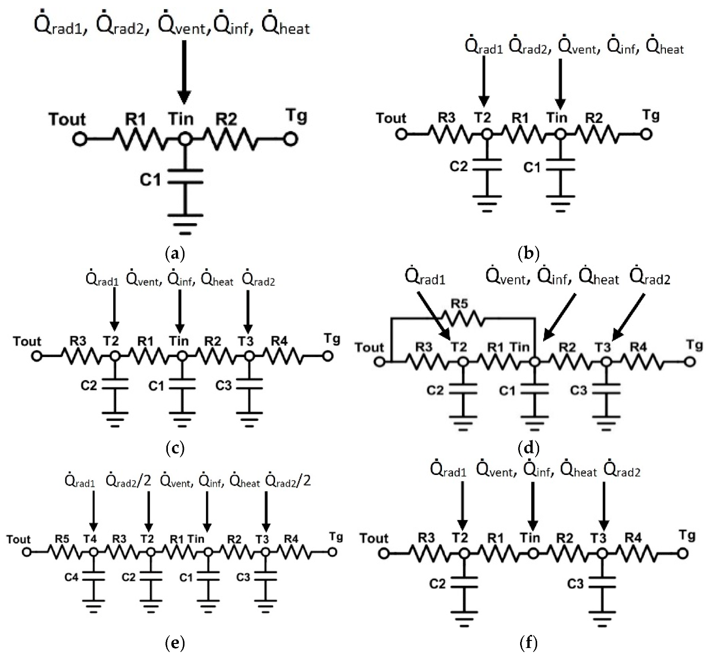
Figure 1 represents all the developed models of a detached building in contact with the outdoor temperature and the ground as the boundary conditions. They evolve from a basic model with 2R1C to a model with 5R4C. The model with 2R1C (M1) represents the envelope with a thermal resistance and the thermal capacitance of the building accumulated in one node. Concurrently, models M2, M3, M4, and M6 use a 2R1C branch to show the envelope and the model M5 uses a 3R2C branch. The model M4 considers an extra resistance to represent windows. Moreover, the branch that connects the indoor temperature to the ground evolved from a simple resistance in model M1 to a 2R1C branch in models M3, M4, M5, and M6.

For the purposes of this work, it is assumed that the heating, ventilation, and infiltration loads are inserted directly into T_in. The solar radiation on the opaque parts ($\dot{Q}$_rad1) is inserted into the external node of the wall structure (T₂ or T₄). Solar radiation is inserted on node T₂ for models M2, M3, M4, and M6, and it is inserted on node T₄ for model M5. The solar radiation through windows ($\dot{Q}$_rad2) is inserted on node T₃ for models M2, M3, M4, and M6. Solar radiation through the windows is divided into two parts on model M5, half of it is heating the node T₃ and half of it is heating node T₂, which is the interior surface of the envelope. Therefore, each model has seven different inputs, including T_out, T_g, $\dot{Q}$_rad1, $\dot{Q}$_rad2, $\dot{Q}$_vent, $\dot{Q}$_inf, and $\dot{Q}$_heat, and 1 output T_in.

It is important to note that the application of RC models for building simulation, using a data-driven approach, is bonded with the available dataset, which is addressed in Section 2.2 and Section 2.3. These input vectors are provided either from a simulation engine like TRNSYS or from the measurements of an experiment/real case study. It is important to know that each of these input vectors (including T_out, T_g, $\dot{Q}$_rad1, $\dot{Q}$_rad2, $\dot{Q}$_vent, $\dot{Q}$_inf, $\dot{Q}$_heat) are time series and that at each time step their value might change. For instance, the outdoor temperature (T_out) of a dataset of 24 h with the time step of one hour will contain 24 elements; consequently, the final input matrix will have 7 columns and 24 rows. If the length of the dataset increases, the number of rows will increase but the number of columns will remain constant as we have considered seven input elements for the input matrix.

2.1.1. State Space Model

The state space representation is employed to write down the formulation of each model. The state of a dynamic system is the set of physical quantities, whose specification (together with the external excitation) completely determines the evolution of the system. If a system is represented with a series of first-order differential equations as shown in Equation (3), where x_i is a state of the system and u_i is an input, e.g., (T_out, T_g, $\dot{Q}$_rad1, $\dot{Q}$_rad2, $\dot{Q}$_vent, $\dot{Q}$_inf, $\dot{Q}$_heat), then Equation (4) shows a general state space representation of the system.

$$\{\begin{array}{c}{\dot{x}}_1=a_{11}\left(t\right)x_1+\cdots +a_{1n}\left(t\right)x_n+b_{11}\left(t\right)u_1+\cdots +b_{1r}\left(t\right)u_r\hfill \\ {\dot{x}}_2=a_{21}\left(t\right)x_1+\cdots +a_{2n}\left(t\right)x_n+b_{21}\left(t\right)u_1+\cdots +b_{2r}\left(t\right)u_r\hfill \\ ⋮\\ {\dot{x}}_n=a_{n1}\left(t\right)x_1+\cdots +a_{nn}\left(t\right)x_n+b_{n1}\left(t\right)u_1+\cdots +b_{nr}\left(t\right)u_r\hfill \end{array}$$

(3)

$$\dot{\mathit{x}}=\mathit{A}\left(t\right)\mathit{x}+\mathit{B}\left(t\right)\mathit{u}$$

(4)

If the A and B matrices in Equation (4) do not depend on time then the system model is called a linear time-invariant (LTI) model, as shown in Equation (5). For applying state space representation for RC models, the coefficients of A and B matrices will be extracted from Equations (1) and (2). Consequently, the states of the RC model will be the temperature variations, as can be seen in Equation (2). In general, Equation (6) is used as the measurement equation. Usually, the measurements (outputs, y) are a function of states, and not the state variations, where a linear correlation between states and the mode output exists in RC models. The coefficients in C and D matrices are independent of matrices A and B, although they are essential to calculating state variations. As the number of states increases, a more complex system is modeled. Considering the thermal network approach, it is clear that this method does not consider every possible state of a building. For instance, the developed models in Figure 1 consider the indoor, envelope, and floor temperatures as the dominant states of the system.

$$\dot{\mathit{x}}=\mathit{A}\mathit{x}+\mathit{B}\mathit{u}$$

(5)

$$\mathit{y}=\mathit{C}\mathit{x}+\mathit{D}\mathit{u}$$

(6)

The general solution of Equation (5) is shown in Equation (7), and the model output is obtainable from Equation (8).

$$\mathit{x}\left(t\right)=e^{\mathit{A}\left(t-t_0\right)}\mathit{x}\left(t_0\right)+{{\displaystyle \int }}_{\tau =t_0}^{\tau =t}{e}^{\mathit{A}\left(t-\tau \right)}\mathit{B}\mathit{u}\left(\tau \right)d\tau$$

(7)

$$\mathit{y}=\mathit{C}{e}^{\mathit{A}\left(t-t_0\right)}\mathit{x}\left(t_0\right)+{{\displaystyle \int }}_{\tau =t_0}^{\tau =t}\mathit{C}{e}^{\mathit{A}\left(t-\tau \right)}\mathit{B}\mathit{u}\left(\tau \right)d\tau$$

(8)

The discrete form of the state space model is shown with Equations (9) and (10). The matrices A_d and B_d can be determined with Euler expansion of Equation (5), where A_d is I + AT_s and B_d is equal to BT_s. T_s is the specified time-step for the model, I is the identity matrix, and k is the time counter.

$$\mathit{x}\left(k+1\right)={\mathit{A}}_d\mathit{x}\left(k\right)+{\mathit{B}}_d\mathit{u}\left(k\right)$$

(9)

$$\mathit{y}\left(k\right)=\mathit{C}\mathit{x}\left(k\right)+\mathit{D}\mathit{u}\left(k\right)$$

(10)

2.1.2. System Identification of LTI Models

Having defined the structure of a model using the thermal network method, the numerical values of its parameters need to be estimated. The system identification approach needs the measured input and output signals, a model structure, and an estimation method to calculate values for the adjustable parameters in the selected model. Therefore, it is possible to represent the system with a state space model and estimate the values of its parameters from datasets. This approach is known as grey-box modeling. The estimation is done by minimizing the error (cost function–the mean square error), as shown in Equation (11), between the model output and the measured data [22].

$$\mathit{V}\left(\theta \right)=\frac{1}{N}{\displaystyle \sum }_{t=1}^N{\mathit{e}}^T\left(\mathit{\theta },t\right)\mathit{e}\left(\mathit{\theta },t\right)$$

(11)

In Equation (11), N is the number of data samples, e(θ,t) is a given error vector at time t and parametrized with θ. Then, parameters are obtainable by minimizing V(θ) with respect to the parameter vector θ. In RC models, vector θ contains the thermal resistances and thermal capacitances of the corresponding model. For instance, model M1 has only three parameters e.g., R1, R2, and C1, and model M3 has seven parameters which are R1, R2, R3, R4, C1, C2, and C3.

The system identification process initiates with an initial guess on parameters. In this work, the initial values of thermal resistances and thermal capacitances are presumed to be R = 0.1 and C = 1000. A first model output (here indoor temperature) is calculated according to the state space representation (Equations (9) and (10)). Next, the model output is compared with the indoor temperatures from the datasets. If the deviation between model outputs and available datasets from TRNSYS and the experiment are large, then the iteration algorithms modify the initial guess, and it continues until the error vector in Equation (11) reaches its threshold, which is set at 0.01. Then, quality matrices will be used to study the quality of the model output in comparison with the available datasets.

The quality of the metrics represents the quality of identified models. In this paper, the normalized mean square error (NRMSE, Equation (12)), also known as “fit percent” and mean square error (MSE, Equation (11)) are used to describe the quality of the identified models.

$$FitPercent=100\times \left(1-\frac{\sqrt{{\left(y_{measured}-y_{model}\right)}^2}}{\sqrt{{\left(y_{measured}-\overline{y_{measured}}\right)}^2}}\right)$$

(12)

The system identification toolbox in Matlab [22] is employed in this work to minimize the cost function in Equation (11) and to estimate model parameters, which are thermal resistances (R) and thermal capacitances (C). The system identification toolbox uses Gauss–Newton, Adaptive subspace Gauss–Newton, Levenberg–Marquardt, or Gradient least squares search to minimize the cost function. The ‘auto’ algorithm, a combination of the line search algorithms, is used for the search method to minimize the cost function and to estimate model parameters. This algorithm determines the optimized trajectory among different techniques at each iteration.

2.2. Building Simulation with TRNSYS

Due to the lack of available data for buildings, some works typically use available software and tools to prepare datasets for special case studies [12,23]. The approach to developing a reliable RC model of a building with a limited number of thermal resistances and capacitances in this study is intended to pave the path toward a district simulation. With regard to this, TRNSYS simulation that is presented here will be used in future works for providing a dataset of buildings with various geometrical features. Therefore, the model type 56 in TRNSYS is used to generate datasets for a simulated office building. The model type 56 [24] uses the Mitalas and Arseneault transfer functions relationships to model the walls, roof, and floor [25,26]. In model type 56, it is possible to determine the energy requirement for zones controlled in an idealized way. Therefore, the heating and cooling energy flow is directly connected to the zone air temperature node. The model type 56, by default, uses the energy level control to calculate the heating/cooling demands. This method is easy to implement but it does not represent the transient behavior of the system from instantaneous changes, while in temperature level control, the room state reflects both the boundary conditions and the instantaneous input effects. In this paper, the linear quadratic regulator (LQR) is used to control the indoor temperature and the application of this approach with the thermal network method is discussed in Section 2.3.

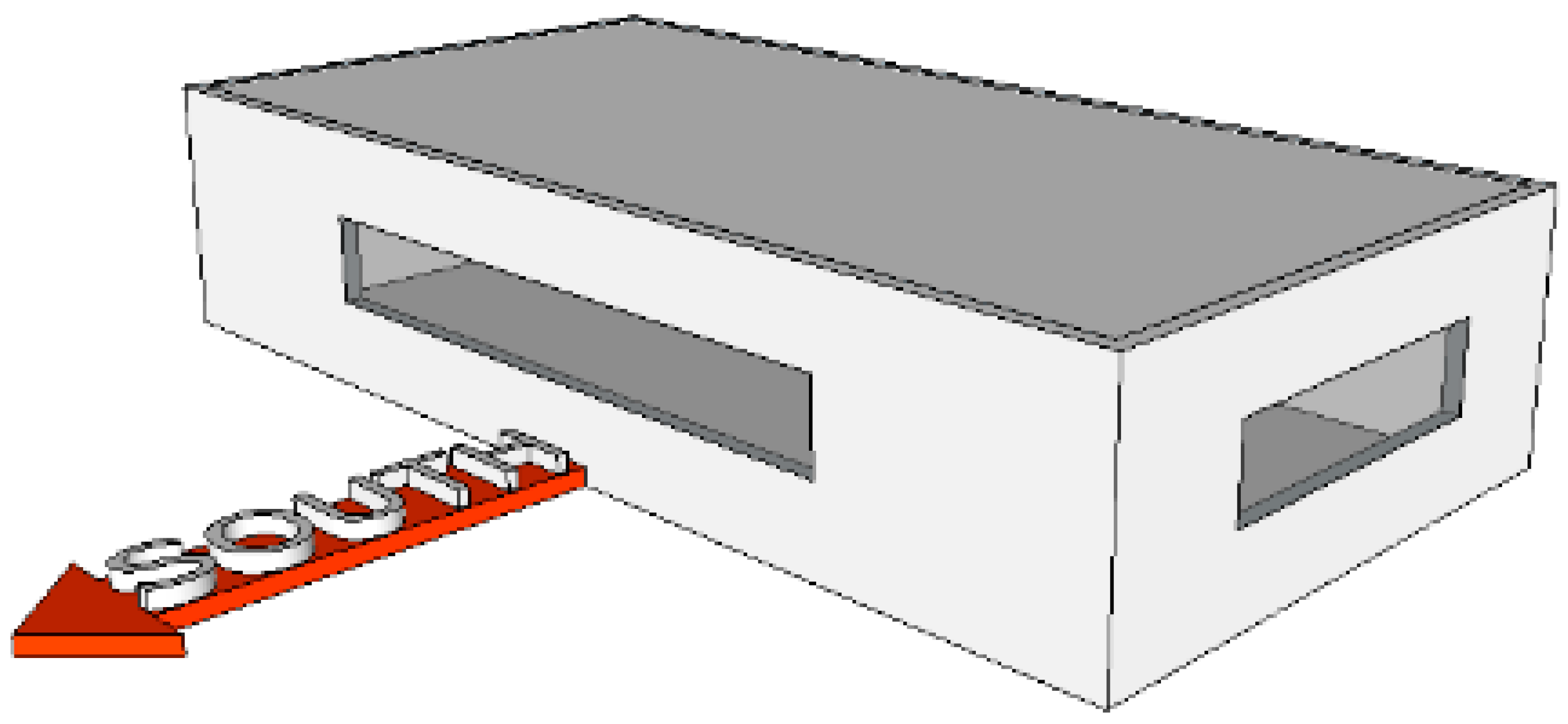
TRNSYS is used to generate a dataset for training the models in Figure 1. For this purpose, a 100 m² detached building with 3 m of height is simulated in TRNSYS. A simple scheme of the building is represented in Figure 2. It is a small office building and the thermal properties of the envelope, including the walls, windows, roof, and floor are given in [27]. The minimum indoor temperature is 15 °C and it occurs between 18:00 to 9:00, and the maximum indoor temperature is 22 °C between 9:00 to 18:00. When the temperature is above 22 °C the heating system turns off and it is assumed that there exists no cooling equipment. The ventilation rate is fixed at 3 ach (air change per hour) during working hours and the rest of the time it is 0.25 ach. It is also assumed that there is no heat recovery system, and the air exchange occurs directly between the indoor air and the ambient. Furthermore, the infiltration rate is assumed to be fixed and equal to 0.24 per hour.

According to Figure 2, the simulated building has the largest window facing south and small windows are placed on the east and west walls. The wall at the back (north facing) has no windows. The roof has no slope. The Uccle meteonorm dataset in TRNSYS provides the necessary information for weather data such as Tout, and the solar radiation for the first 1000 h, beginning from January 1st. With a simple calculation, the solar radiation is divided into two parts, i.e., one part heats the opaque part of the envelope and the other part passes through the windows ($\dot{Q}$_rad1 and $\dot{Q}$_rad2). The ground temperature is assumed to be fixed and it is equal to 10 °C. Figure 3 represents the results from the TRNSYS simulation for the indoor temperature and Figure 4 represents the calculated heating load in TRNSYS.

2.3. Real Building Measurements

The other dataset used in this study stems from a real building that is constructed as part of the project IEA annex 58 [21]. The Twin Houses N2 and O5 in Holzkirchen, Germany, were tested and detailed measurements of the indoor and weather conditions are provided to be used for system identification. It is shown that the two houses have almost the same heating load profile to keep the set temperatures. The detailed information about the building location, geometry, construction, and conducted experiments is provided in the manual [28].

The tested building contains nine thermal zones, including attic, cellar, living room, corridor, kitchen, bathroom, hallway, and two bedrooms, as shown in Figure 5. The available datasets contain detailed measurements such as indoor temperature, humidity ratio, heat demand, infiltration, and ventilation rates of each zone. The weather data is also measured on site, including outdoor temperature, global solar radiation on each orientation, ground temperature, wind speed, and humidity ratio.

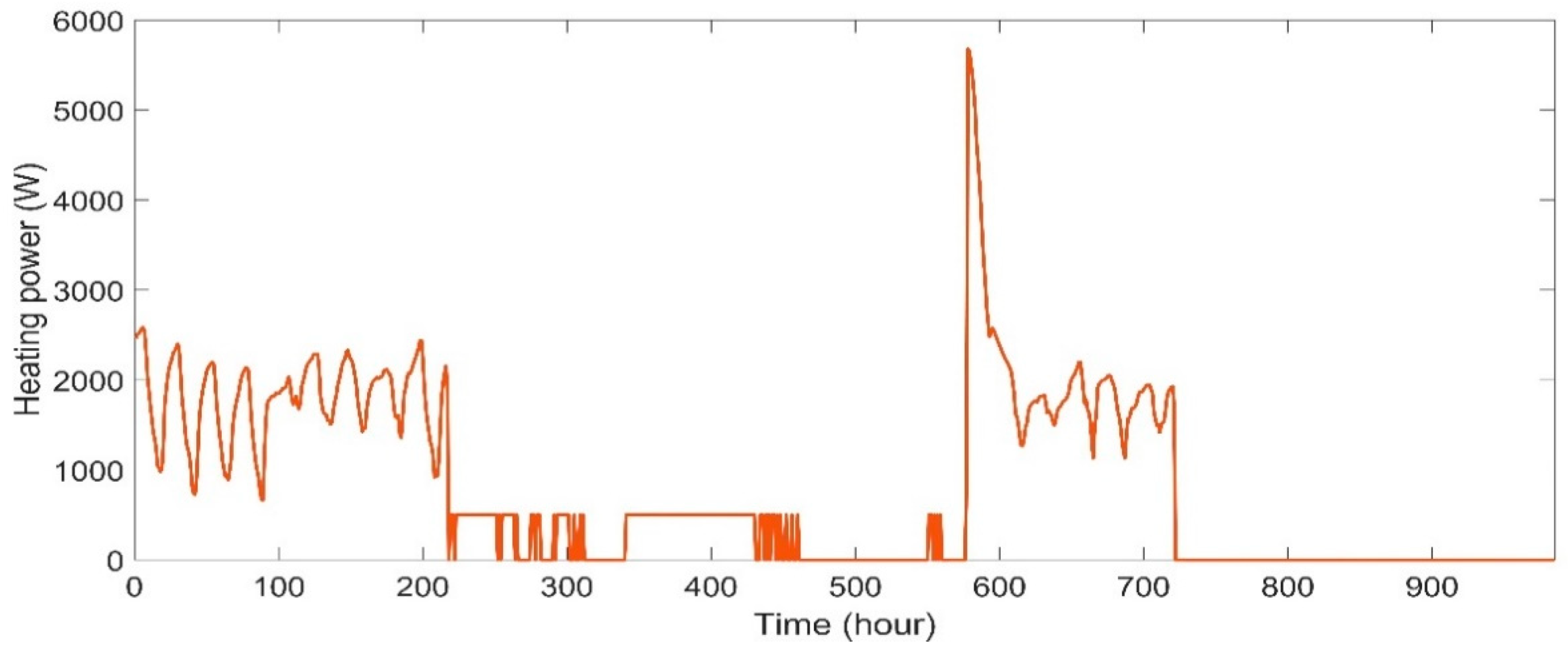
To prepare the dataset for system identification, some simplifications are made. First, the multi-zone building is considered as a single zone, assuming that the indoor temperature is the volume average temperature of all zones except the cellar. Second, the cellar temperature is used as a boundary condition for the simulated thermal zone, and it is considered as the ground temperature T_g. The heat consumptions in every zone are summed together and are used as the heat input in the dataset. The solar radiation, infiltration, and ventilation are treated like the TRNSYS data. With these considerations, the indoor temperature and the heat power for the real building are represented in Figure 6 and Figure 7 respectively.

According to Figure 6 and Figure 7, the indoor temperature was fixed at 28 °C for the first period of the experiment, which lasted for nine days. The second part of the experiment studied the effects of constant heat input with different frequencies on the indoor temperature and then the heating system was shut down and the building free temperature was measured. Next, the fourth week of the experiment started with a set temperature of 22 °C and it caused a jump in the heat power. The constant indoor temperature lasted for one week and again the building’s free temperature was measured for the last week of this experiment. It is important to note that the measured data until 575 h (before the heat jump) has been used for the system identification and the rest of the data has been used for model validation at constant indoor temperature.

Here it is important to note that RC models have been used by researchers [29] for cooling load calculations too. However, heating load calculations have been studied as the provided experimental data is for the heating season. Thus, the TRNSYS simulation is also adjusted for the heating load calculation. Due to the seasonality of the estimated parameters of RC models, it is not possible to use the same set of parameters for calculating heating loads for the determination of cooling load in buildings. At the end of this section, we summarize the system identification process as it is shown in Figure 8.

On the left side of the presented scheme there is the generated dataset form TRNSYS/experiment. On the right side, it can be seen how the system identification iteration process is established to estimate the parameters, which provides the corresponding model output in comparison to the available datasets.

2.4. Controller Design and Linear Quadratic Regulator (LQR) Technique

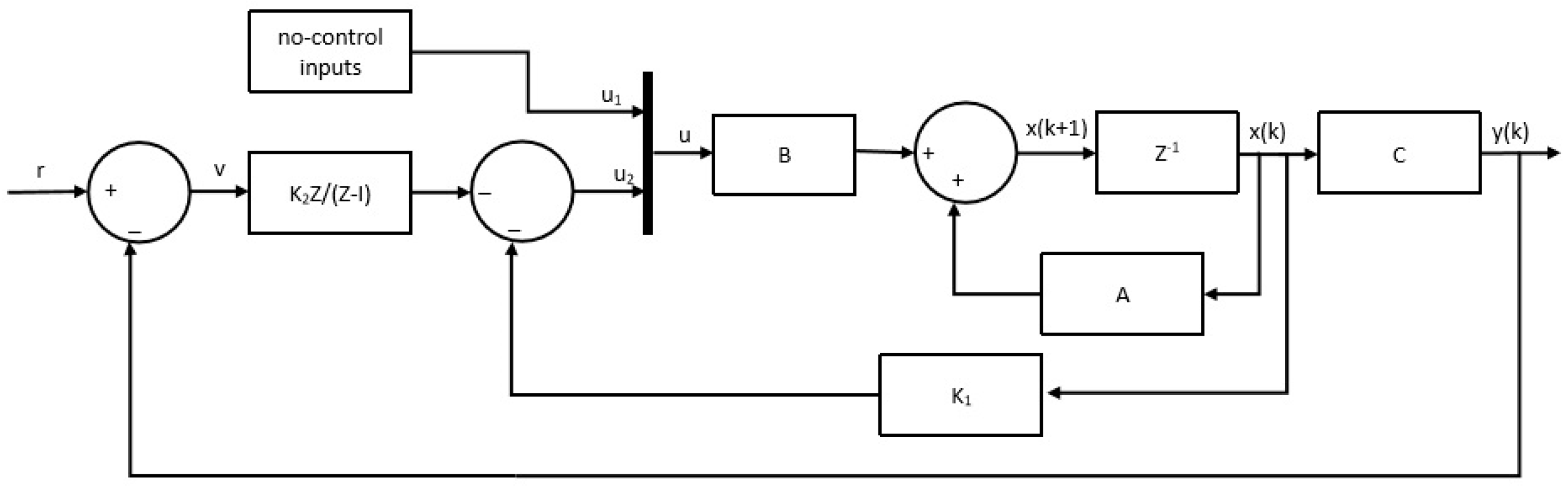
Using the LQR approach can provide realistic results because it includes the transient behavior of the system such as time lags for determining the energy demand. The classic control strategies such as PID controller design and pole placement method are mainly suitable for SISO (Single-Input Single-Output) system that is mainly presented with transfer functions [30]. Using the thermal network method and specifying the different states of the system enables the use of advanced control techniques. Therefore, a more generic solution is to use output feedback and state feedback for tracking the reference indoor temperature [31], where K₁ and K₂, in Figure 9, are calculated by means of the LQR method.

To calculate K₁ and K₂, it is important to re-write the state space model to include the feedback loops. Therefore, the discrete state space matrices in Equations (9) and (10) are replaced with the augmented matrices in Equation (13) to Equation (18), and the augmented state space representation is shown in Equations (19) and (20). The heating load is calculated from the states and output feedbacks of the system as shown in Equation (18).

$${\mathit{x}}^{*}=\left[\begin{array}{c}\mathit{x}\\ \mathit{v}\end{array}\right]$$

(13)

$${\mathit{A}}^{*}=\left[\begin{array}{cc}\mathit{A}& \mathbf{0}\\ -\mathit{C}\mathit{A}& \mathit{I}\end{array}\right]$$

(14)

$${\mathit{B}}^{*}=\left[\begin{array}{c}\mathit{B}\\ -\mathit{C}\mathit{B}\end{array}\right]$$

(15)

$${\mathit{E}}^{*}=\left[\begin{array}{c}\mathbf{0}\\ \mathit{I}\end{array}\right]$$

(16)

$${\mathit{C}}^{*}=\left[\begin{array}{cc}\mathit{C}& \mathbf{0}\end{array}\right]$$

(17)

$$\mathit{u}=-\left[\begin{array}{cc}{\mathit{K}}_1& {\mathit{K}}_2\end{array}\right]\left[\begin{array}{c}\mathit{x}\\ \mathit{v}\end{array}\right]$$

(18)

$${\dot{\mathit{x}}}^{*}={\mathit{A}}^{*}{\mathit{x}}^{*}+{\mathit{B}}^{*}\mathit{u}+{\mathit{E}}^{*}\mathit{r}$$

(19)

$$\mathit{y}={\mathit{C}}^{*}{\mathit{x}}^{*}$$

(20)

A quick and accurate technique to determine K₁ and K₂ is to use the LQR (linear quadratic regulator) method, which is defined in the scope of the optimal control strategies [32]. Optimal control is a control method that minimizes (or maximizes) a well-chosen cost function or performance index. In the LQR technique, the cost function (J) for the infinite horizon has a general form as shown in Equation (21), where x is the state vector, and u is the input vector. In addition, Q is a positive semidefinite matrix that penalizes the departure of system states from the equilibrium, and R is a positive definite matrix that penalizes the control input.

$$J=\frac{1}{2}{\displaystyle \sum }_{k=0}^N\left({\mathit{x}}^{\mathit{T}}\left(k\right)\mathit{Q}\mathit{x}\left(k\right)+{\mathit{u}}^{\mathit{T}}\left(k\right)\mathit{R}\mathit{u}\left(k\right)\right)$$

(21)

The aim is to find the sequence for the input vector u that minimizes the cost function J. This problem can be tackled by introducing Lagrange multipliers and by defining an augmented cost function that leads to determining u as shown in Equation (22). K is derived from the minimization of Equation (21) and it can be calculated according to Equation (23). The matrix P in Equation (23) can be determined from Equation (24) [32,33]. With this approach, it is possible to use the developed model with the thermal network method in a closed loop to control the indoor temperature. It must be noted that the controller gains (K₁ and K₂) are calculated for the heating load, and therefore the solar radiation, outdoor temperature, ventilation, infiltration, and ground temperatures are considered as known inputs and they have been directly introduced inside the model.

$$\mathit{u}\left(k\right)=-\mathit{K}\mathit{x}\left(k\right)$$

(22)

$$\mathit{K}={\left[\mathit{R}+{\mathit{B}}^{\mathit{T}}\mathit{B}\right]}^{-1}{\mathit{B}}^{\mathit{T}}\mathit{P}\mathit{A}$$

(23)

$$\mathit{P}=\mathit{Q}+{\mathit{A}}^{\mathit{T}}\mathit{P}\mathit{A}-{\mathit{A}}^{\mathit{T}}\mathit{P}\mathit{B}{\left[\mathit{R}+{\mathit{B}}^{\mathit{T}}\mathit{P}\mathit{B}\right]}^{-1}{\mathit{B}}^{\mathit{T}}\mathit{P}\mathit{A}$$

(24)

3. Results

As already pointed out, the main objective of this paper is to search among different thermal network structures to find the one which determines the indoor temperature and heating load with high accuracy and at the same time has good accuracy to represent the thermal properties of the structure. In this context, the system identification results for the simulated building in TRNSYS as well as for the measured data of the real building are presented.

3.1. System Identification and Model Response for the Simulated Building in TRNSYS

The six different thermal network structures (shown in Figure 1) are trained with the obtained results from TRNSYS simulations. The higher values for FitPercent and smaller values for MSE are performance indicators that are used in this work to describe the quality of the identified models. It can be concluded that not every proposed model is suitable for identifying the desired output signal (indoor temperature). According to Figure 10 and

Table 1. Goodness of fit and MSE for each identified model compared to TRNSYS training dataset.

Model	Goodness of Fit	MSE Temperature
M1	−117.5%	42.51
M2	−24.87%	17.71
M3	70.87%	0.76
M4	42.19%	3.37
M5	69.94%	0.81
M6	38.33%	6.72

, models M1, M2, M4, and M6 failed to identify the indoor temperature accurately. The calculated FitPercent (see Equation (12)) for these models is less than 50% and confirms the low quality of the identified models. On the other hand, models M3 and M5 appear more promising. Models M3 and M5 identified the output signal with around 70% accuracy and the mean square errors (MSE) for these models are 0.76 and 0.81 °C², respectively. According to the calculated MSE, it can be concluded that models M3 and M5 are more suitable for identifying the indoor temperature with the considered observed inputs and output.

In addition to the good quality of the models M3 and M5 in identifying the indoor temperature, it is also important that the model determines the heat demand with high accuracy compared to TRNSYS results. For this purpose, the LQR technique is used to make the closed loop of the building for determining the required heating load to track the indoor temperature for 1000 h from the 1st of January. The outputs of each thermal network are compared with simulated results in TRNSYS in

Table 2. Model output in a closed loop to track indoor temperature for TRNSYS.

Model	MaxT (°C)	RMSE T (°C)	Max $\dot{Q}$ (W)	Error $\dot{Q}$	Total Q (Wh)	Error Q
TRNSYS	22.00		13,442.7		604,354.1
M1	33.58	6.55	26.27	99.80%	4808.7	99.20%
M2	30.74	8.49	264.64	98.03%	48,383.6	92.00%
M3	23.75	1.06	13,572.4	0.96%	634,304.3	4.95%
M4	35.47	5.02	22,479.7	67.22%	725,814.5	20.09%
M5	23.35	0.70	13,205.2	1.76%	656,666.2	8.65%
M6	30.63	3.08	0.0	100.0%	0.00	100%

.

As expected, models M1, M2, M4, and M6 cannot determine the maximum temperature, the maximum heat power, and the total heat demand accurately, given that they already failed to identify the indoor temperature. On the other hand, models M3 and M5 determined the maximum heat power with a maximum error of 2% compared to TRNSYS results, and the total heat demand during the simulation period is determined with a maximum error of 8.65%. Although model M4 calculates the total heat demand with 20% of error compared to TRNSYS simulations, it fails to determine the maximum temperature and peak power accurately. The comparison between the calculated heat demand from model M3 and the simulated results from TRNSYS is shown in Figure 11.

Based on the above analysis, it can be concluded that models M3 and M5 are reliable models for determining the indoor temperature and heat demand for the simulated building in TRNSYS. These two models, M3 and M5, identify the indoor temperature with high accuracy, the MSE is less than 1 °C², and the determined heat demands have also good accordance with simulated results from TRNSYS. The last performance indicator that is important in this work are the thermal properties of the structure.

In this context, the main indicator to represent the building’s thermal properties is the UA value, which is known as the overall heat loss coefficient of the envelope. In this study, the UA_e value represents the UA value of the building structure that includes walls and roof, and the UA_f value represents the UA value of the floor. If the thermal network method gives a good estimation of the UA values of the envelope, then it can be assumed that the model determines the total heat demand with a high accuracy.

Table 3. Identified parameters and calculated UA value of each model from the TRNSYS dataset.

Parameter	Units	TRNSYS	M1	M2	M3	M4	M5	M6
R1	°C/W		1.0000	0.0437	0.0120	1.0000	0.0053	0.7110
R2	°C/W		0.0003	0.0013	0.0016	0.0011	0.0019	0.0016
R3	°C/W			0.0188	0.0002	1.0000	0.0055	0.7146
R4	°C/W				0.0223	0.0002	0.9661	0.0001
R5	°C/W					0.0130	0.0001
C1	Wh/°C	815.2	4160.9	1733.4	662.8	697.6	671.2
C2	Wh/°C	5580.6		7059.8	3578.8	1000.0	1000.0	1370.1
C3	Wh/°C	18,355.2			22,058.0	13,394.0	18,558.0	4557.1
C4	Wh/°C						234,022.7
UAe value	W/°C	66.22	1.00	16.01	81.77	77.33	91.90	0.70
UAf value	W/°C	17.18	3486.76	798.37	41.73	788.53	1.03	562.15

presents the identified values for the parameters in each thermal network.

Accordingly, the estimated UA values for models M1, M2, and M6 are far from the calculated one, which is obtained from the material properties of the structure. The calculated UA values from TRNSYS libraries are 66.22 W/°C and 17.18 W/°C, respectively. When these values are compared with the estimated values from models M3, M4, and M5, the calculated errors are 23.4%, 16.7%, and 38.7% respectively for the UA_e value. According to Table 3, the UA_f value has not been estimated as accurately as the UA_e value. The best result is achieved from model M3 with an error of around 150%. On the other hand, it is clear that the thermal capacitances have not been estimated as accurately as the UA values. According to Table 3, model M3 estimated the thermal capacitances with a lower error compared to models M4 and M5.

In Table 3, although we observe a deviation between estimated UA values of M3 and M5 with the TRNSYS calculations, these models are still capable of determining the heating load demand with less than 10% error. It will be shown that when experimental data are used, the estimated UA values with these two models remain more accurate than the calculated values from physical properties, which make them suitable for further applications. Besides, the deviations between estimated UA values and the calculated UA values from the physical properties of the envelope come from the different approaches to determining these parameters. In TRNSYS, UA value is calculated by means of physical parameters of the envelope materials, while in RC models lumped parameters and data-driven techniques are used that by default estimate these parameters with less information than using physical properties.

3.2. System Identification and Model Response for the Real Building

For the sake of completeness, it is necessary to validate the proposed methodology for measured data of the real building described in Section 2.3. The identification was performed with the measured data during the first two periods. Thus, the closed-loop response to determining the heating power starts from the beginning of the third period. The comparison between the measured data and the FitPercent of each identified model is presented in Figure 12 and

Table 4. Goodness of fit and MSE for each identified model compared to the training dataset for the real building.

Model	Goodness of Fit	MSE Temperature
M1	−45.07%	17.56
M2	87.25%	0.14
M3	91.87%	0.06
M4	83.24%	0.25
M5	88.74%	0.11
M6	52.50%	1.92

. Except for models M1 and M6, all other proposed models identify the output signal with more than 80% of FitPercent. The goodness of fit of more than 80% leads to the maximum MSE of 0.25 in model M4. Due to the small values of FitPercent and large values of MSE in model M1, it can be concluded that this model is not suitable for further analysis.

After the identification part, the parameters in each model have been estimated. These models can be used to compute the indoor temperature and heating load for the next period, when the indoor temperature is set to 22 °C, and when the models are set in a closed loop for tracking the indoor temperature. It can be seen in

Table 5. Model output in a closed loop to track indoor temperature for the real building.

Model	MaxT (°C)	RMSE T (°C)	Max $\dot{Q}$ (W)	Error $\dot{Q}$	Total Q (Wh)	Error Q
Measured	22.34		5680.792		29,9553.5
M2	18.05	5.87	963.63	83.04%	76,550.37	74.45%
M3	23.32	0.78	6802.80	19.75%	381,039.12	27.20%
M4	26.25	1.65	8460.94	48.94%	337,977.11	12.83%
M5	23.49	0.94	7317.18	28.81%	364,091.45	21.54%
M6	17.73	11.35	0.00	100%	0.00	100%

that model M2 fails to calculate the maximum temperature and heating load with high accuracy, although it succeeded in getting more than 80% of FitPercent in identifying indoor temperature. On the other hand, models M3, M4, and M5 determine the total heat demand with an error of around 25% compared to the measured data. Models M3 and M5 determine the maximum heat power with 20% and 28% of error. In fact, model M4 determines the maximum heat power with an almost 50% of error that is too large to be considered a reliable result. Additionally, model M4 also calculates a maximum indoor temperature of 26 °C that confirms that this model is not suitable for further applications. Thus, models M3 and M5 have the best responses among the examined models in identifying the output signal and determining the maximum heat power and total heat demand.

In this context, Figure 13 presents the predicted indoor temperature and Figure 14 shows the calculated heat demand for the next week of the real building by means of the M3 model. During the simulation period, the indoor temperature is fixed at 22 °C for 6 days in row. Accordingly, the model M3 determines the indoor temperature with high accuracy, although it overestimates the heat demand.

The last part of the analysis is to examine the accuracy of identified models compared to the building’s thermal properties. The building’s structure properties are tabulated in [28]. It has been assumed that the total heat transfer coefficients for outdoor and indoor air regimes are 8 and 23 (W/m²K), and these values are used to calculate the UA value of the building by means of the measured data. With this assumption, the UAe value (walls and roof) is almost 114.39 W/K and the UAf value becomes 27.04 W/K.

According to

Table 6. Identified parameters and calculated UA value of each model for the real building.

Parameter	Units	Building	M1	M2	M3	M4	M5	M6
R1	°C/W		0.10000	0.00711	0.00695	0.10000	0.00073	0.10000
R2	°C/W		0.00012	0.00503	0.00089	0.00038	0.00120	0.00187
R3	°C/W			0.00042	0.00001	0.00079	0.00739	0.02137
R4	°C/W				0.00554	0.00273	0.00395	0.00020
R5	°C/W					0.01734	0.00006
C1	Wh/°C	3578.9	11,492.0	19,000.6	2058.8	2246.8	2200.7
C2	Wh/°C	10,895.5		1311.5	40,774.9	1000.0	14,960.1	1101.2
C3	Wh/°C	20,000			24,276.6	8846.1	1000.0	2784.6
C4	Wh/°C						9870.4
UAe value	W/°C	114.93	10.00	132.80	143.68	67.59	122.25	8.24
UAf value	W/°C	27.04	8333.33	198.81	155.52	321.54	194.17	483.09

, the estimated UAe value for model M4 is much less than what was expected from the envelope properties. On the other hand, M3 and M5 estimate the UAe value with 25% and 6.3% of error compared to the envelope’s thermal properties. Thus, it can be concluded that besides the good representation of the building’s thermal performance, models M3 and M5 also estimate the thermal properties of the building with high accuracy. Model M3 contains fewer parameters than model M5, but also it does not estimate the total heat demand and UA value as accurately as model M5 does. On the other hand, model M5 has the best performance in determining indoor temperature, maximum and total heating load, and it estimates the UAe value with higher accuracy. Still, more considerations are required to model the thermal branches between the indoor air and the ground.

4. Discussion

In this paper, different structures of thermal networks are used to simulate a detached building with the ground temperature as a boundary condition. The complexity of the thermal networks evolves from a 2R1C up to a 5R4C model. It was shown that a model with at least three thermal capacitances can identify the indoor temperature with high accuracy, and an RMSE of 1 °C is achievable when the goodness of fit is more than 60%.

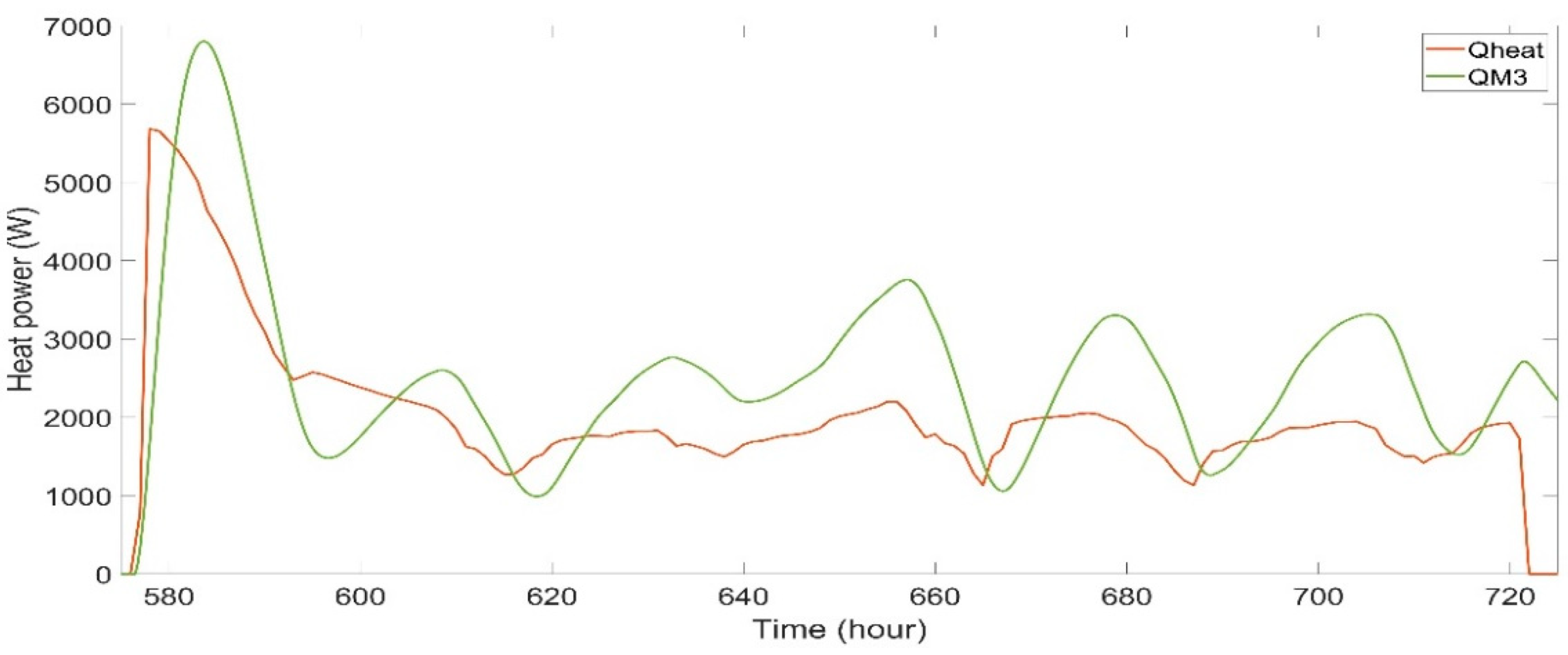
Moreover, it was shown that models M3 and M5 are able to estimate the UA_e value of the simulated building with deviations up to 23.4% and 38.7%, and the UA_e value of a real building with 25% and 6.3% of deviation compared to the calculated UA_e value from the material properties. These two models also give a better response to determining the load demand when they are used in a closed loop system and the feedback gains are calculated with the LQR technique. It can be seen that the 4R3C (M3) and 5R4C (M5) models estimate the maximum heating power with around 25% error compared to measured data, while the 5R4C (M5) model estimates the total heat demand with 20% of excess compared to real measurements for the constant indoor temperature of 22 °C.

In this context, the M3 and M5 models, using 2R1C and 3R2C branches for the envelope and a 2R1C branch for the floor, are rather sufficient to identify the indoor temperature and to determine the heat dynamics. Although model M5 displays a better performance either for load estimation or UA value calculation, it uses one more resistance and capacitance compared with model M3, which leads us to retain model M3 as the simplest structure that can be used in a building energy management system.

5. Conclusions

This paper examines the simplest thermal network structure to model a detached residential building. The model is coupled with the control system that determines the indoor temperature, total heat demand during the simulation period, the maximum heat power, and the UA value with high accuracy. It can be concluded that the model with at least three thermal capacitances is sufficient to identify the indoor temperature. Using more thermal capacitances increases the model accuracy to determine the heat dynamics and the UA value. In addition, it was shown that coupling the thermal network method and the control system, by means of the LQR technique, is an expeditious method to determine the heat dynamics of buildings. This approach gives results as accurate as the energy level control technique in TRNSYS. Future work may be directed toward the development of small neighborhood models based on the proposed modeling approach, while the building’s geometry effects on the model parameters can pave the way for using this as a reference model for district energy management systems.

References

1. Tardioli, G.; Kerrigan, R.; Oates, M.; Donnell, J.O.; Finn, D. Data driven approaches for prediction of building energy consumption at urban level. Energy Procedia 2015, 78, 3378–3383. [Google Scholar] [CrossRef] [Green Version]
2. Roth, J.; Rajagopal, R. Benchmarking building energy efficiency using quantile regression. Energy 2018, 152, 866–876. [Google Scholar] [CrossRef]
3. Hassid, S. A linear model for passive solar calculations: Evaluation of performance. Build. Environ. 1985, 20, 53–59. [Google Scholar] [CrossRef]
4. Seem, J.E. Modeling of Heat Transfer in Buildings; The University of Wisconsin-Madison: Madison, WI, USA, 1987. [Google Scholar]
5. Yang, S.; Pilet, T.J.; Ordonez, J.C. Volume element model for 3D dynamic building thermal modeling and simulation. Energy 2018, 148, 642–661. [Google Scholar] [CrossRef]
6. Fraisse, G.; Viardot, C.; Lafabrie, O.; Achard, G. Development of a simplified and accurate building model based on electrical analogy. Energy Build. 2002, 34, 1017–1031. [Google Scholar] [CrossRef]
7. Park, H.; Ruellan, M.; Martaj, N.; Bennacer, R.; Monmasson, E. Generic thermal model of electrical appliances in thermal building: Application to the case of a refrigerator. Energy Build. 2013, 62, 335–342. [Google Scholar] [CrossRef]
8. Xu, X.; Wang, S. A simplified dynamic model for existing buildings using CTF and thermal network models. Int. J. Therm. Sci. 2008, 47, 1249–1262. [Google Scholar] [CrossRef]
9. Evins, R. A review of computational optimisation methods applied to sustainable building design. Renew. Sustain. Energy Rev. 2013, 22, 230–245. [Google Scholar] [CrossRef]
10. Bagheri, A.; Feldheim, V.; Ioakimidis, C.S. On the evolution and application of the thermal network method for energy assessments in buildings. Energies 2018, 11, 890. [Google Scholar] [CrossRef] [Green Version]
11. Bacher, P.; Madsen, H. Identifying suitable models for the heat dynamics of buildings. Energy Build. 2011, 43, 1511–1522. [Google Scholar] [CrossRef]
12. Reynders, G.; Diriken, J.; Saelens, D. Quality of grey-box models and identified parameters as function of the accuracy of input and observation signals. Energy Build. 2014, 82, 263–274. [Google Scholar] [CrossRef]
13. Andersen, K.K.; Madsen, H.; Hansen, L.H. Modelling the heat dynamics of a building using stochastic differential equations. Energy Build. 2000, 31, 13–24. [Google Scholar] [CrossRef] [Green Version]
14. Jiménez, M.J.; Madsen, H.; Andersen, K.K. Identification of the main thermal characteristics of building components using MATLAB. Build. Environ. 2008, 43, 170–180. [Google Scholar] [CrossRef]
15. Jiménez, M.J.; Porcar, B.; Heras, M.R. Application of different dynamic analysis approaches to the estimation of the building component U value. Build. Environ. 2009, 44, 361–367. [Google Scholar] [CrossRef]
16. ISO 13790:2008; Energy Performance of Buildings—Calculation of Energy Use for Space Heating and Cooling. International Organization for Standardization: Geneva, Switzerland, 2008. Available online: https://www.iso.org/standard/41974.html (accessed on 10 March 2008).
17. VDI-Verein Deutscher Ingenieure e.V., VDI-Guideline-VDI 6007/3 “Calculation of Transient Thermal Response of Rooms and Buildings; Modelling of Solar Radiation”|Build Up, The Association of German Engineers. 2012. Available online: http://www.buildup.eu/en/practices/publications/vdi-guideline-vdi-60073-calculation-transient-thermal-response-rooms-and (accessed on 5 June 2012).
18. Lauster, M.; Teichmann, J.; Fuchs, M.; Streblow, R.; Mueller, D. Low order thermal network models for dynamic simulations of buildings on city district scale. Build. Environ. 2014, 73, 223–231. [Google Scholar] [CrossRef]
19. Vivian, J.; Zarrella, A.; Emmi, G.; de Carli, M. An evaluation of the suitability of lumped-capacitance models in calculating energy needs and thermal behaviour of buildings. Energy Build. 2017, 150, 447–465. [Google Scholar] [CrossRef]
20. Wang, S.; Xu, X. Parameter estimation of internal thermal mass of building dynamic models using genetic algorithm. Energy Convers. Manag. 2006, 47, 1927–1941. [Google Scholar] [CrossRef]
21. Janssens, A. Reliable Building Energy Performance Characterisation Based on Full Scale Dynamic Measurements in Buildings Background; EBC Annex 58; International Energy Agency: Ghent, Belgium, 2016. [Google Scholar]
22. Ljung, L. System Identification Toolbox TM Getting Started Guide R 2015 a How to Contact MathWorks; The MathWorks, Inc.: Natick, MA, USA, 2015. [Google Scholar]
23. Ogunsola, O.T.; Song, L.; Wang, G. Development and validation of a time-series model for real-time thermal load estimation. Energy Build. 2014, 76, 440–449. [Google Scholar] [CrossRef]
24. Kummert, M. Trnsys 16, A Transient System Simulation Program. 2007. Available online: http://sel.me.wisc.edu/trnsys/ (accessed on 7 March 2007).
25. Stephenson, D.G.; Mitalas, G.P. Calculation of Heat Conduction Transfer Functions for Multi-Layer Slabs. 1971. Available online: http://nparc.cisti-icist.nrc-cnrc.gc.ca/npsi/jsp/nparc_cp.jsp?lang=frL’accèsàcesiteWebetl’utilisationdesoncontenusontassujettisauxconditionsprésentéesdanslesitehttp://nparc.cisti-icist.nrc-cnrc.gc.ca/npsi/jsp/nparc_cp.jsp?lang=en (accessed on 2 October 2018).
26. Mitalas, G.P.; Arseneault, J.G. FORTRAN IV Program to Calculate Z-Transfer Functions for the Calculation of Transient Heat Transfer through Walls and Roofs, Ottawa. 1972. Available online: https://nrc-publications.canada.ca/eng/view/ft/?id=9a383a07-6830-401d-a3a7-ab15ad077208 (accessed on 30 August 2022).
27. Bagheri, A.; Feldheim, V.; Thomas, D.; Ioakimidis, C.S. Coupling building thermal network and control system, the first step to smart buildings. In Proceedings of the IEEE 2nd International Smart Cities Conference: Improving the Citizens Quality of Life, ISC2, Trento, Italy, 12–15 September 2016. [Google Scholar] [CrossRef]
28. Strachan, P.; Heusler, I. Twin Houses Empirical Dataset: Experiment 1; University of Strathclyde: Glasgow, UK, 2015. [Google Scholar] [CrossRef]
29. Ji, Y.; Xu, P.; Duan, P.; Lu, X. Estimating hourly cooling load in commercial buildings using a thermal network model and electricity submetering data. Appl. Energy 2016, 169, 309–323. [Google Scholar] [CrossRef]
30. Katsuhiko, O. Modern Control Engineering, 5th ed.; Pearson: Hoboken, NJ, USA, 2010. [Google Scholar]
31. Kim, D.; Cai, J.; Braun, J.E.; Ariyur, K.B. System identification for building thermal systems under the presence of unmeasured disturbances in closed loop operation: Theoretical analysis and application. Build. Environ. 2016, 107, 169–180. [Google Scholar] [CrossRef] [Green Version]
32. Albertos, P.; Sala, A. Multivariable Control Systems: An Engineering Approach; Springer: London, UK, 2004. [Google Scholar] [CrossRef]
33. Lavretsky, E.; Wise, K.A. Robust and Adaptive Control; Springer: Berlin/Heidelberg, Germany, 2013. [Google Scholar] [CrossRef]
Figure 1. Series of thermal networks for simulating the indoor temperature of a detached building: (a) M1: 2R1C; (b) M2: 3R1C; (c) M3: 4R3C; (d) M4: 5R3C; (e) M5:5R4C; (f) M6: 4R2C.
Buildings 12 01625 g001
Figure 2. Schematics of a simple simulated building in TRNSYS.
Buildings 12 01625 g002
Figure 3. Indoor temperature for a 100 m2 building simulated in TRNSYS.
Buildings 12 01625 g003
Figure 4. Determined heat power for a 100 m2 building simulated in TRNSYS.
Buildings 12 01625 g004
Figure 5. Twin house [28]: (a) cross-section; (b) ground floor plan.
Buildings 12 01625 g005
Figure 6. Measured indoor temperature for a building calculated from presented data in [28].
Buildings 12 01625 g006
Figure 7. Measured heat power for a building calculated from the presented data in [28].
Buildings 12 01625 g007
Figure 8. A scheme of implementation of the system identification technique for the parameter estimation of RC models based on the available datasets from TRNSYS simulations and experiment.
Buildings 12 01625 g008
Figure 9. Closed loop of the system for tracking the indoor temperature by introducing an integrator and splitting the feedback gain.
Buildings 12 01625 g009
Figure 10. Comparison between identified models and the building simulated by TRNSYS.
Buildings 12 01625 g010
Figure 11. Calculated heat demand from model M3 and the simulated results from TRNSYS.
Buildings 12 01625 g011
Figure 12. Comparison between identified models and the training dataset for the real building.
Buildings 12 01625 g012
Figure 13. Comparison between the simulated indoor temperature and measured data for the real building by means of Model M3.
Buildings 12 01625 g013
Figure 14. Comparison between the simulated heat power and measured data for the real building by means of model M3.
Buildings 12 01625 g014