Big Data-Based Performance Analysis of Tunnel Boring Machine Tunneling Using Deep Learning

Abstract

In tunnel boring machine (TBM) construction, the advance rate is a crucial parameter that affects the TBM driving efficiency, project schedule, and construction cost. During the operation process, various types of indicators that are monitored in real-time can help to control the advance rate of TBM. Although some studies have already been carried out in advance rate prediction, the research is almost all based on statistical methods and shallow machine learning algorithms, thereby having difficulties in dealing with a very large amount of monitored data and in modeling the time-dependent characteristics of the parameters. To solve this problem, a deep learning model is proposed based on the CNN architecture, bidirectional Long Short-Term Memory module, and the attention mechanism, which is called the CNN-Bi-LSTM-Attention model. In the first step, the monitored data is processed, and the CNN architecture is adopted to extract features from the data sequence. Then the Bi-LSTM module is adopted to obtain the time-dependent indicators. The significant features can be addressed by the added attention mechanism. In the model training process, the rotation speed of the cutter head (N), thrust (F), torque (T), penetration rate (P), and chamber earth pressure (Soil_P) are adopted to predict the advance rate. The influence of the training periods on the model performance is also discussed. The result shows that not only the data amount, but also the data periods have an influence on the prediction. The long-term data may lead to a failure of the advance rate of TBM. The model evaluation result on the test data shows that the proposed model cannot predict the monitored data in the starting stage, which denotes that the working state of TBM in the starting stage is not stable. Especially when the TBM starts to work, the prediction error is big. The proposed model is also compared with several traditional machine methods, and the result shows the excellent performance of the proposed model.

1. Introduction

With the development of city construction, tunnel boring machines (TBMs) have been widely applied in civil engineering. The TBM is a type of mechanization equipment with the characteristics of high efficiency, environment friendly, and safety [1], which are widely used in mine tunneling engineering, hydraulic engineering, subway construction, etc. In the process of TBM operation, the divers control the cutter head and the advance speed by inputting the related parameters. However, it is hard to tune the parameters in a timely manner and making good decisions is based on experience, which may lead to low construction efficiency and cutter wear. The TBM sensors should monitor different kinds of operational parameters, such as rotation speed of cutter, thrust of cutter head, torque of cutter head, advance velocity, and penetration index. These parameters reflect the real-time interaction state of the tunnel face and the cutter head. Based on the recorded data, the TBM performance and driving parameters can be reasonably predicted. It is beneficial to develop an appropriate tunneling plan, minimize the frequency of common risks, and improve the drilling system efficiency in construction [2,3].

Many achievements in TBM performance prediction have been gained from previous studies, and some theoretical and experience-based models have been proposed [4,5,6] to reveal the inner mechanism of TBM operations and establish the relationship between different variables. Sapigni et al. [7] found that the rate of penetration (ROP) is related to the rock mass rating (RMR) based on the data from three tunnels. The relationship of the two parameters can be expressed as a quadratic polynomial regression equation. Kahraman et al. [8] established a regression model for ROP based on the monitored data. The result showed that ROP is determined by the rock properties. Hassanpour et al. [9] built an empirical formula according to multi geo-parameters for ROP based on the data from the NO. 2 Tunnel of Nowsood. It is thought that ROP is closely related to rock mass properties, especially for the field penetration index (FPI). The research also showed that the common indexes applied in rock mass evaluation, such as uniaxial compressive strength (UCS) and rock quality designation (RQD), are convenient for building the prediction model. However, the experience-based model is established for a specific engineering. Hence, the model’s application is limited.

Some researchers also applied numerical simulation in the TBM operation process. Kasper and Meschke [10] analyzed the influence of TBM operational parameters on the foundation using a 3D finite element simulation model. Gong and Zhao [11] analyzed the interaction of the tunnel face and the cutter head using a numerical simulation method, and the result shows that ROP advanced with the growth of the degree of rock brittleness. Li et al. [12] applied the discrete element method (DEM) to analyze the relationship between ROP and wedge angle and confinement stress, and the result showed that large wedge angle lead to tensile cracks and lowers the ROP. Although the numerical models are inspiring for TBM performance prediction, there are also weaknesses in TBM operation analysis. The boundary condition of the model is usually simplified in most cases of numerical simulation calculation. The results of these methods are not accurate and cannot show the minor differences in TBM operational parameter changes.

With the advancement of data science, the intelligent analysis of complex data in engineering projects can be realized. The machine learning methods applied in engineering can improve efficiency and lower cost [13]. Based on the monitoring of data in real projects, intelligent techniques are also applied in TBM operating parameters prediction. Sun et al. [14] combined geological data with the operational data and applied random forest to predict TBM load. Random forest [15] and support vector regression (SVR) [16] with parameters optimization were also applied to predict TBM advance rate and penetration rate, respectively. Noori et al. [17] discussed the factors influencing TBM performance prediction using neural networks and particle swarm optimization (ANN-PSO). Afradi et al. [18] applied fuzzy logic to predict TBM penetration rate, with the optimization algorithm of harmony search and particle swarm. However, it is hard for the shallow networks, such as SVR and random forest, to deal with a very large amount of monitored data in TBM construction. Meanwhile, the time series characteristics of TBM operation data are not considered in establishing the prediction model.

In recent years, deep learning theory has been developed in unstructured data analysis [19,20,21], especially for images and language. It is a subset of artificial neural networks of machine learning. Deep learning models usually have more layers and are deeper than shallow networks. The specific applications of deep learning models include image interpretation [22,23], sound classification [24,25], and text analysis [26,27]. These complex models applied in research are essentially extensions of the simple deep models, such as recurrent neural networks (RNNs) [28], convolutional neural networks (CNNs) [29], deep belief networks [30], and auto-encoder networks [31]. Deep learning models are widely used in engineering, such as dam displacement prediction [32,33], dredging construction operation [34], and mechanical responses prediction of caisson foundation [35]. Some of the models were also applied in TBM performance prediction [36,37,38]. Among these models, RNNs is a special type of network that can output the targets by considering both the previous and current information, thus having advantages in analyzing time series data. However, traditional RNNs suffer from the effects of gradients vanishing or exploding when dealing with long sequences. Therefore, the long short-term memory (LSTM) networks [39] were proposed to improve the RNNs performance. The three types of gates in LSTM, i.e., the input gate, the forget gate, and the output gate, control the data flow in the LSTM unit. The LSTM-based models are also applied in TBM performance prediction. Liu et al. [40] applied LSTM with a global attention mechanism to predict tunnel lithology based on big TBM data. Gao et al. [41] established a LSTM-based model to predict TBM operatingchange parameters and verified the model with a large amount of data collected from a practical project. Fu and Zhang [42] considered spatio-temporal feature fusion in a LSTM model, and conducted a global sensitivity analysis for TBM performance prediction. Li et al. [43] combined CNNs and LSTM to establish the prediction model and analyzed the TBM cutter head speed and penetration rate. However, it is difficult to deal with complex high-dimensional tunneling parameters using the maximum likelihood and classic artificial intelligence (AI) techniques, and the prediction accuracy needs to be improved.

Inspired by the previous achievements, a novel deep learning model was established by combining CNNs and LSTM for the prediction task of TBM performance. The one-dimensional CNNs and the bidirectional LSTM (Bi-LSTM) were adopted to build the whole model. The local and global information is considered in the CNNs, and the time series information is involved in the Bi-LSTM. The significant features are addressed using the attention mechanism. Meanwhile, how much data should be used to build a TBM advance rate is another challenging issue, as deep learning is a totally data-driven approach. In the research, five models were built to address the problem. Moreover, the traditional machine learning methods and the proposed algorithm were also compared. The results showed that the LSTM-based model outperforms the traditional machine learning models. The terms of monitored data are also discussed, and the results show that long-term data may lead to a prediction failure of the TBM advance rate.

2. Methodology

TBM performance prediction is a significant problem in engineering. It is a dynamic process that needs operators to make quick and accurate operational parameter decisions. In the research, the CNN-Bi-LSTM-Attention model was established to predict the advance rate of TBM. The monitored data, including the rotation speed of the cutter head (N), thrust (F), torque (T), penetration rate (P), and chamber earth pressure (Soil_P), were adopted to build the model. The model architecture is shown in Figure 1. The flow chart of the research is as follows.

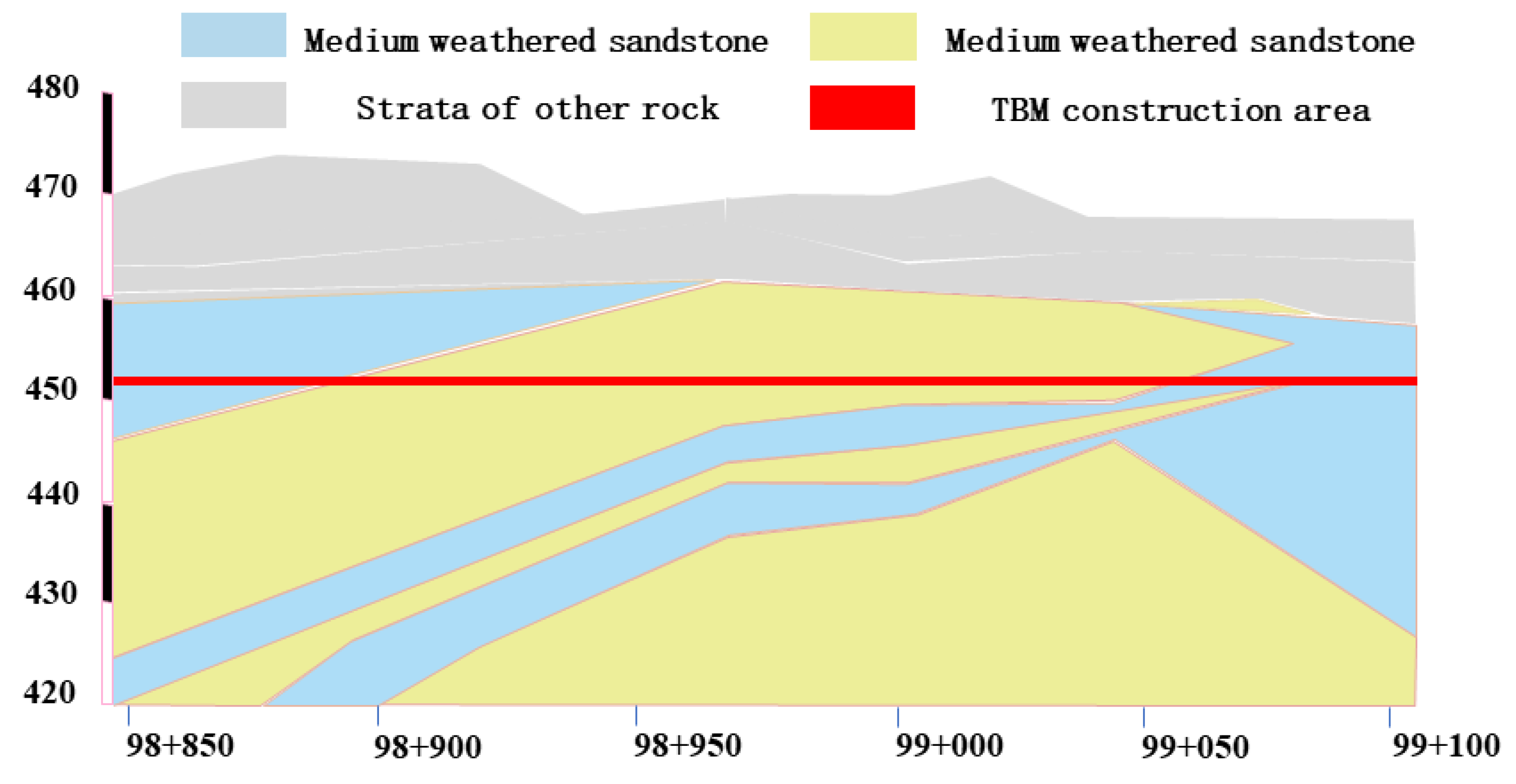
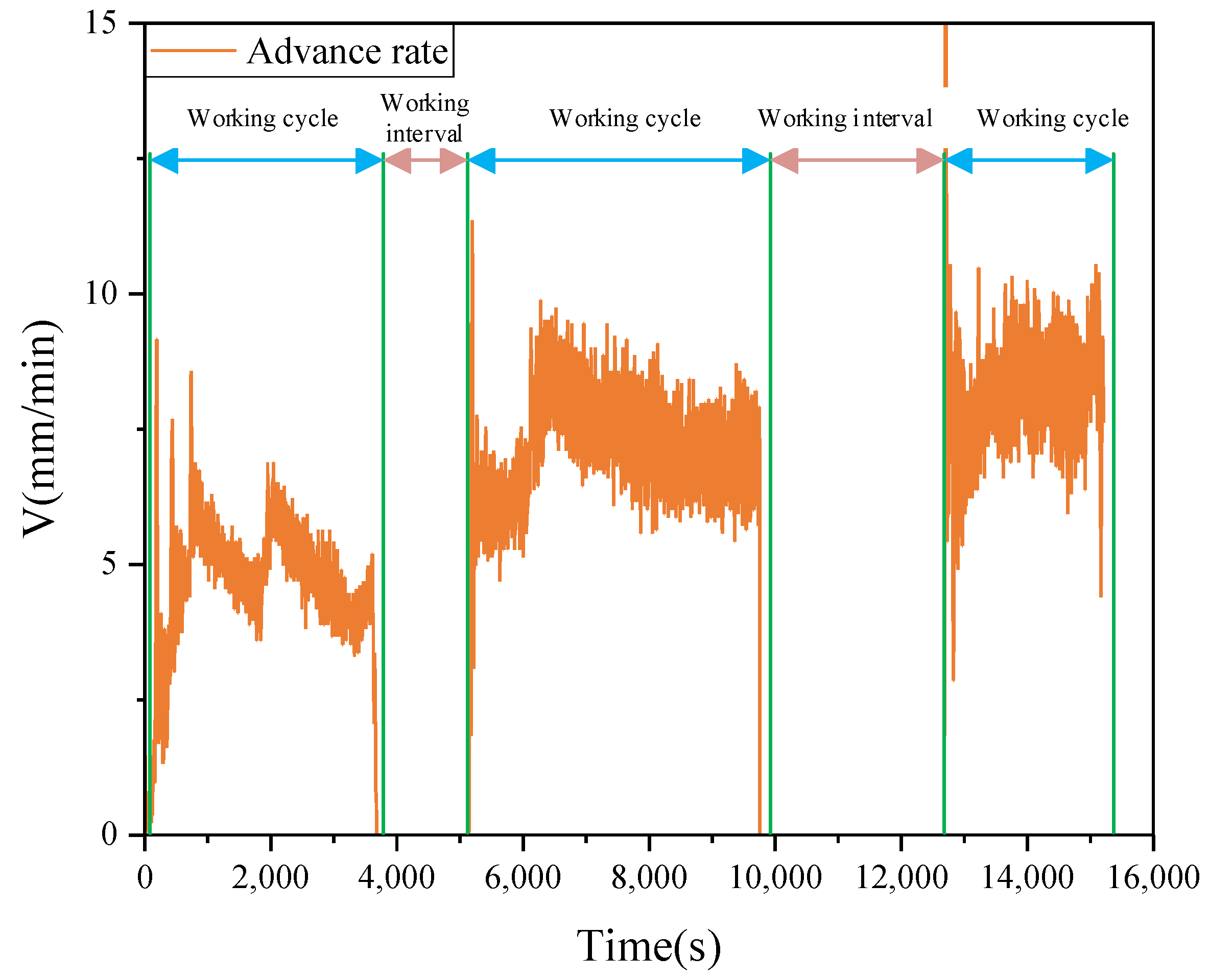
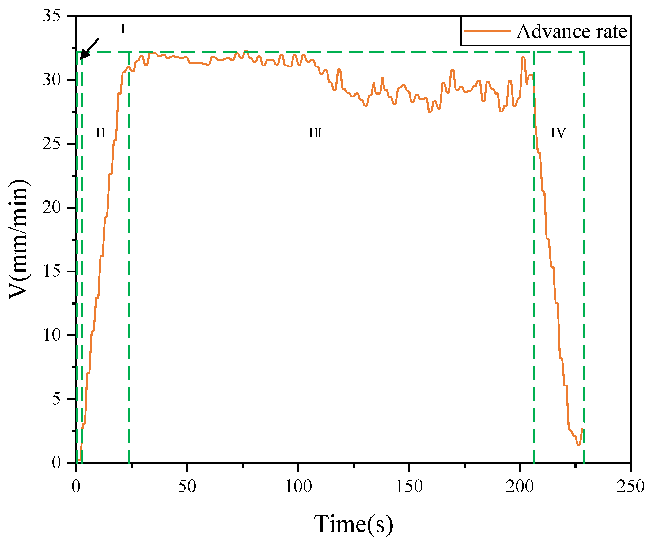
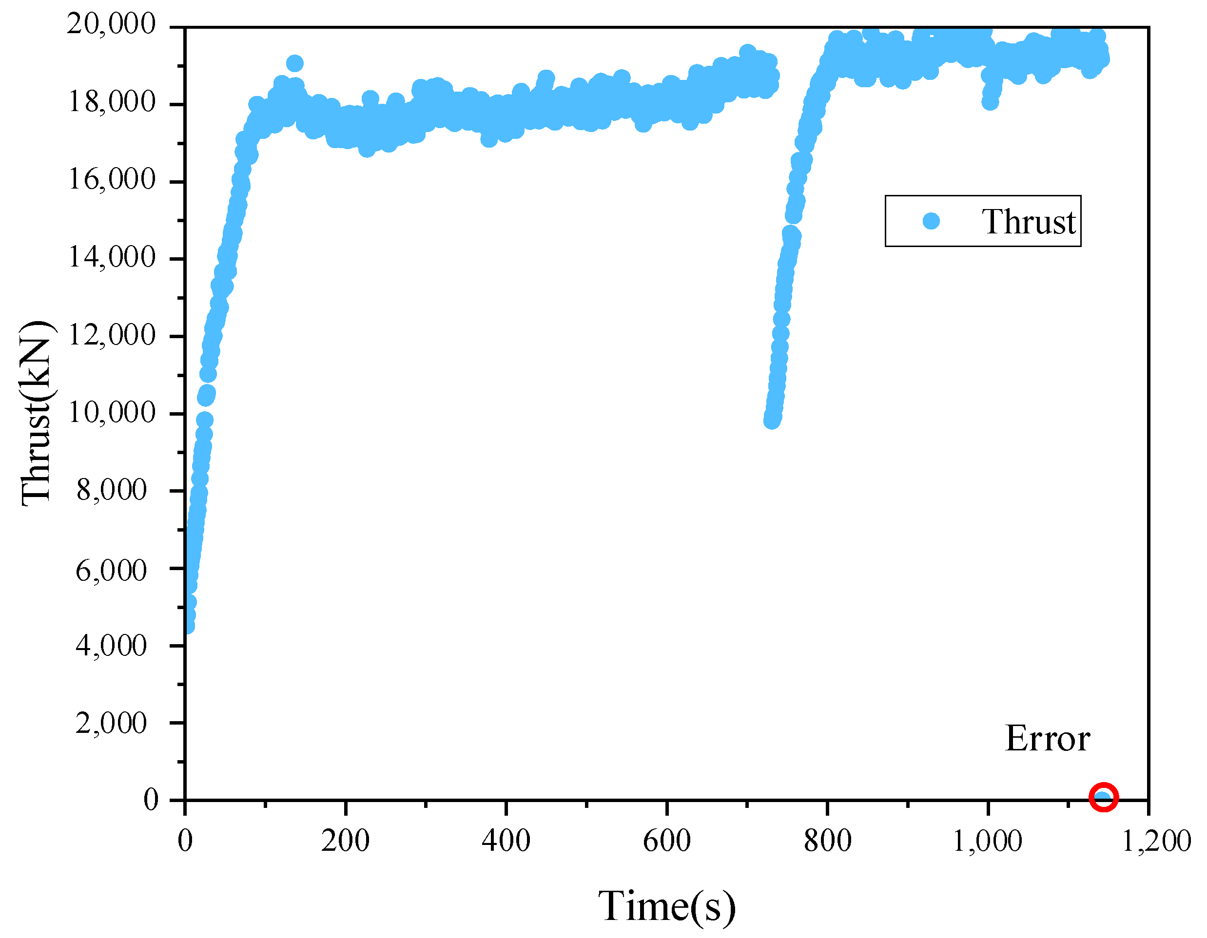
• In step 1, the monitored data was collected using different types of sensors installed on the TBM. The construction data in the strata of medium-weathered sandstone was adopted to train the model. The monitored data sequence for free rotation was also cut in the working process. The error in the monitored data was also detected, and the errors in the data sequence were processed. Normalization was also adopted to scale the data into the range of (0,1).
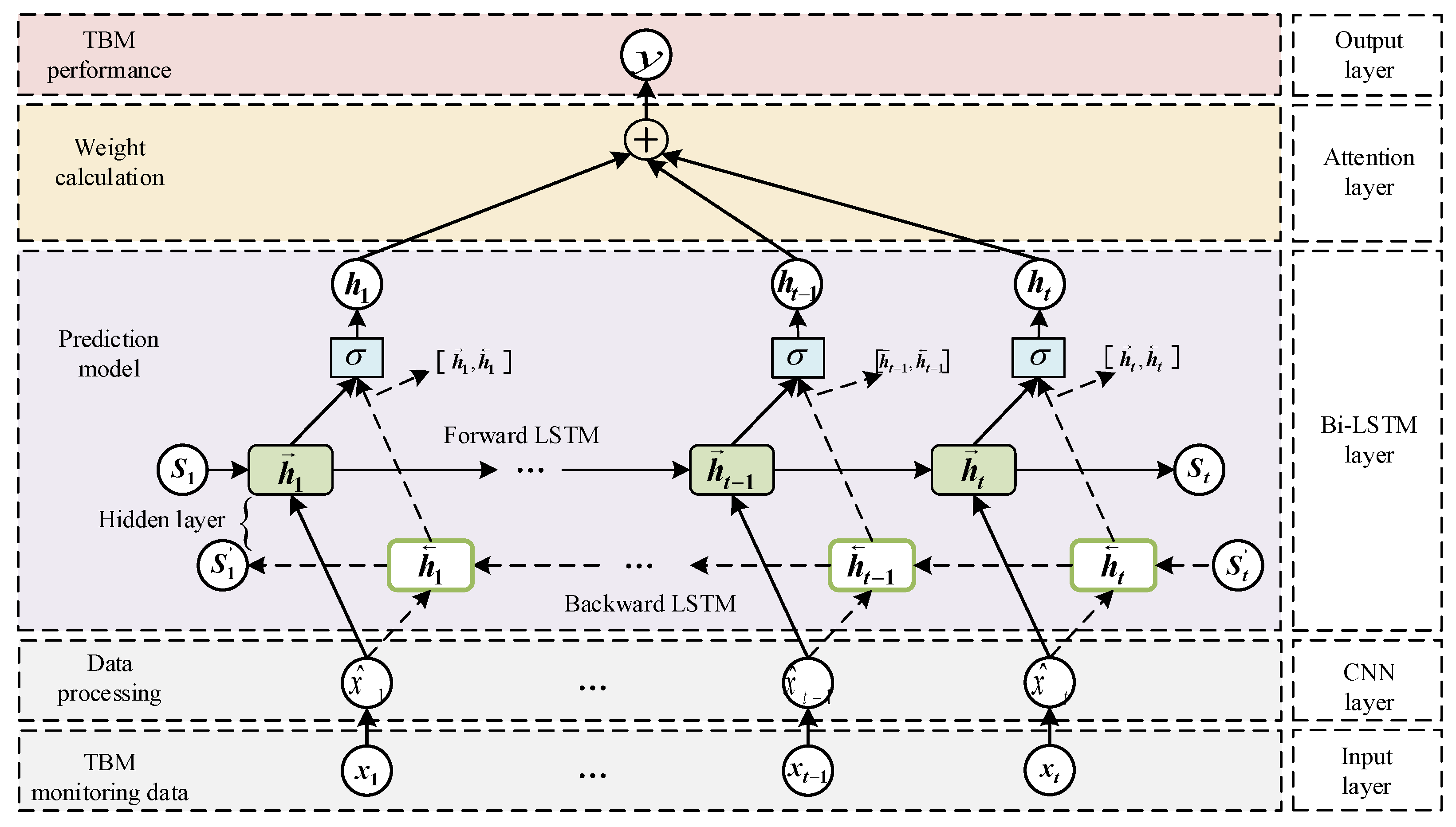
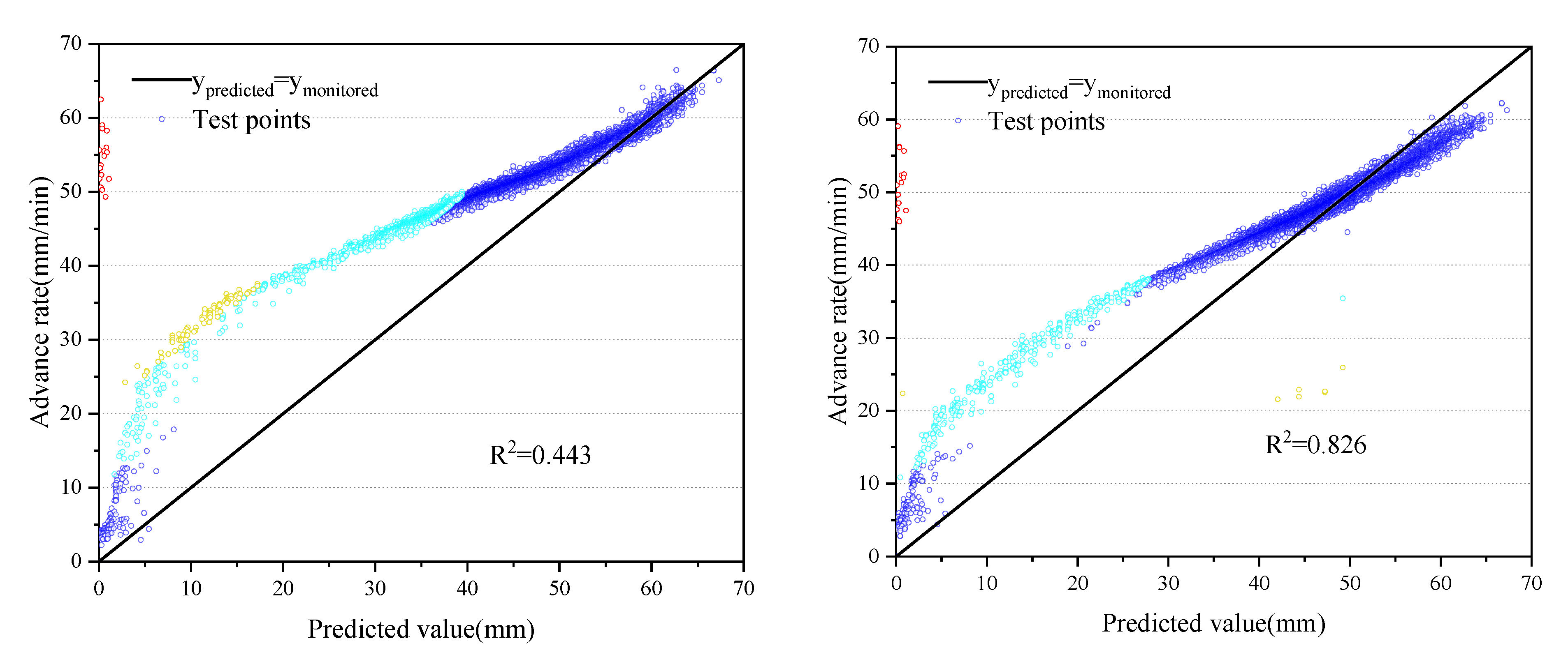
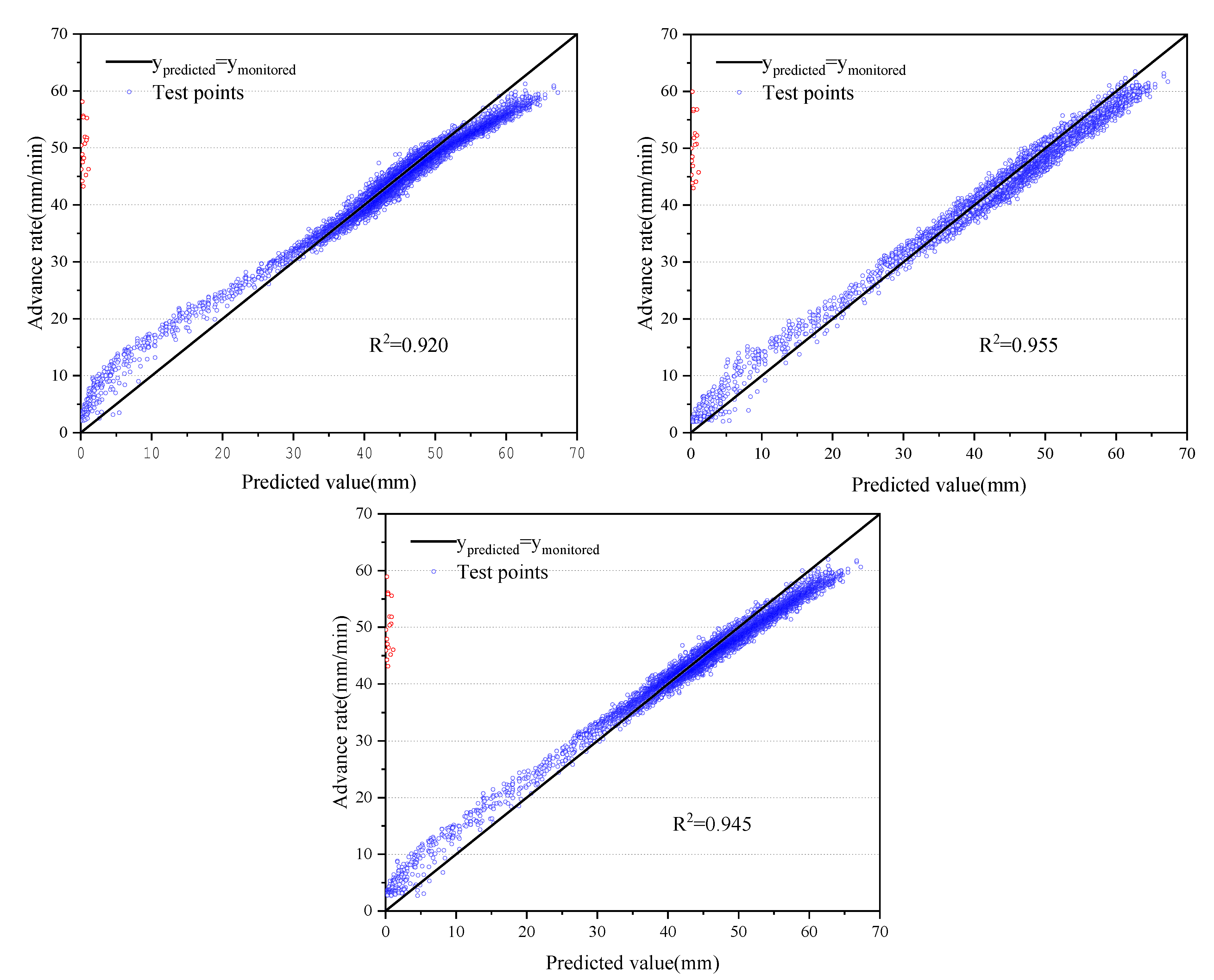
• In step 2, the CNN-Bi-LSTM-Attention model was established using the CNN architecture, bidirectional Long Short-Term Memory module, and the attention mechanism. The CNN architecture was adopted to extract global features from the data sequence. The Bi-LSTM module was adopted to get the time-dependent features. The attention mechanism was used to address the local features, which was significant for the TBM advance rate prediction. Root mean square error (RMSE), Mean absolute error (MAE), and R² were used to evaluate the models. The comparison of the predicted result and the monitored data are also shown.
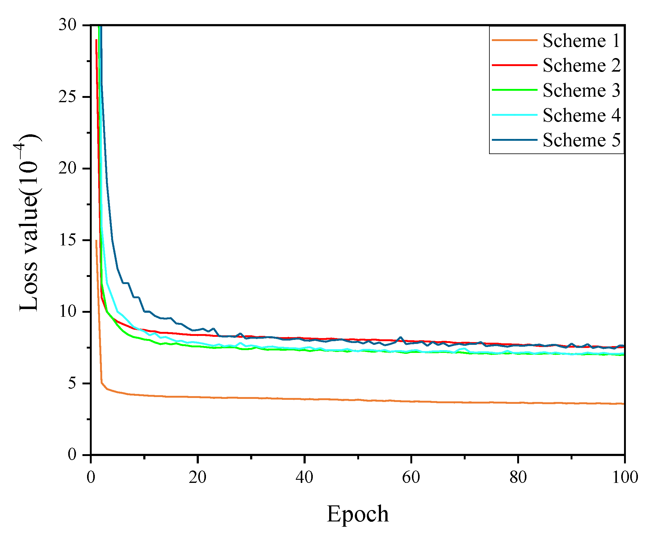
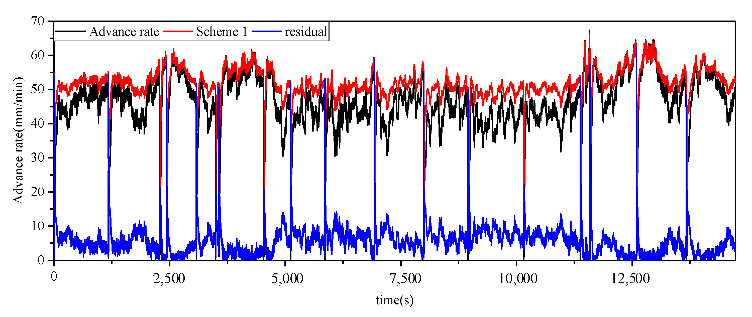
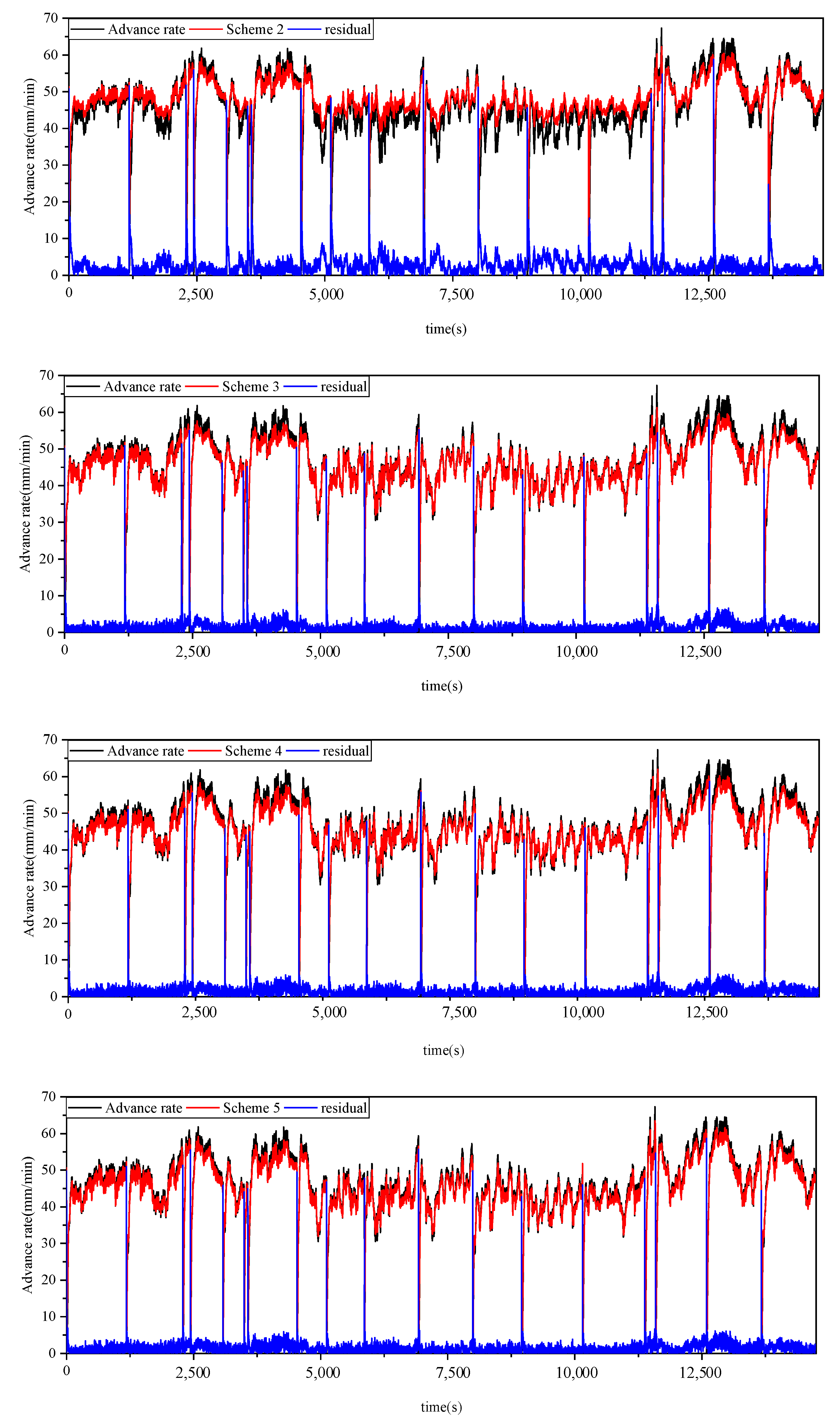
• In step 3, the monitored data from Day 1 to Day 27 was applied. The monitored data of Day 27 were taken as the test data. The training data periods were considered in model training. The data of Day 1-Day 26, Day 20-Day 26, Day 24-Day 26, Day 25-Day 26, and Day 26 were used to train the model. The different schemes of model training were used to evaluate the effectiveness of the data amount and periods. The comparison between the monitored advance rate and the predicted values shows the performance of the different models and where the errors appear in the corking cycle of the TBM.

Finally, the performance of the traditional machine learning methods and the proposed model were compared. The results showed that the proposed model outperforms the traditional models. It indicates that the monitored data of TBM working cycles is time-dependent. The CNN-Bi-LSTM-Attention model can utilize multiple types of features in advance rate prediction.

2.1. CNN

Convolutional neural networks (CNN) have been widely used in image classification, identification, and segmentation tasks, which perform better than traditional image processing methods. The low and high-level features are extracted and integrated to be new features for image analysis. There are three significant ideas for CNN architecture.

• Local connection: The kernels of the CNN layer are only connected to specific ones of the previous layer, which can obtain the effective features of the sequence.
• Weight sharing: The feature map of the input sequence is processed by the same kernel using sliding windows. Therefore, all the neurons of the same kernel share the same parameters, which reduces the time of the training process.
• Pooling layers: Pooling denotes some or all features based on the values. It is implemented in the low- and high-level features integration process.

In this research, the one-dimensional CNN is applied to process the monitoring data. The sequence features are extracted from the sequence through a CNN structure which contains two convolutional layers.

2.2. Bi-LSTM-Attention

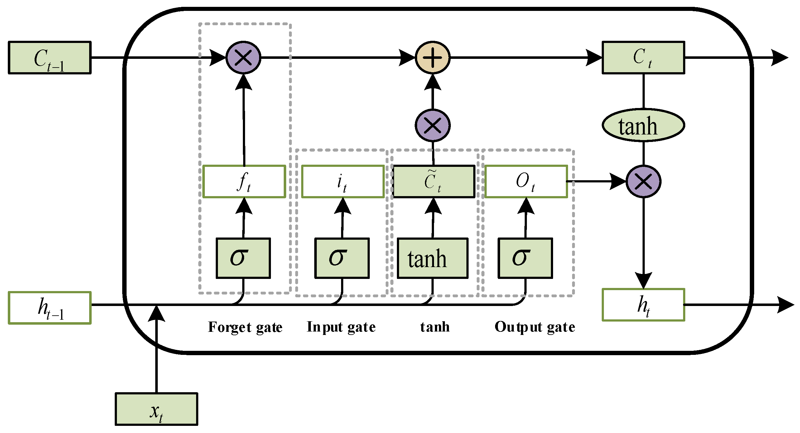
2.2.1. Long Short-Term Memory (LSTM)

LSTM is a kind of RNN architecture with feedback connections. The memory unit in a LSTM network makes it available for information learning over a long period. A common LSTM block includes the input gate, the output gate, and the forget gate in a single unit, as shown in Figure 2. The information transmission is controlled by the three gates in the LSTM block. The three gates in the LSTM block make it possible to solve gradient return problems, including gradient vanishing and exploding. At time t, every gate produces a variable, i_t, f_t, and o_t for the memory c_t. The output of the block is h_t. The hidden state h_t−1 determines the amount of information from x_t to c_t. The variable f_t determines the amount of stored information in cell state c_t−1. The variable o_t controls the final output, h_t. The specific formulae of LSTM are shown in Equations (1)–(5).

$$f_t=\sigma \left(W_f\cdot \left[h_{t-1},x_t\right]+b_f\right)$$

(1)

$$i_t=\sigma \left(W_i\cdot \left[h_{t-1},x_t\right]+b_i\right)$$

(2)

$$o_t=\sigma \left(W_o\cdot \left[h_{t-1},x_t\right]+b_o\right)$$

(3)

$$C_t=f_t\odot C_{t-1}+i_t\odot \tanh \left(W_c\cdot \left[h_{t-1},x_t\right]+b_c\right)$$

(4)

$$h_t=O_t\odot \tanh \left(C_t\right)$$

(5)

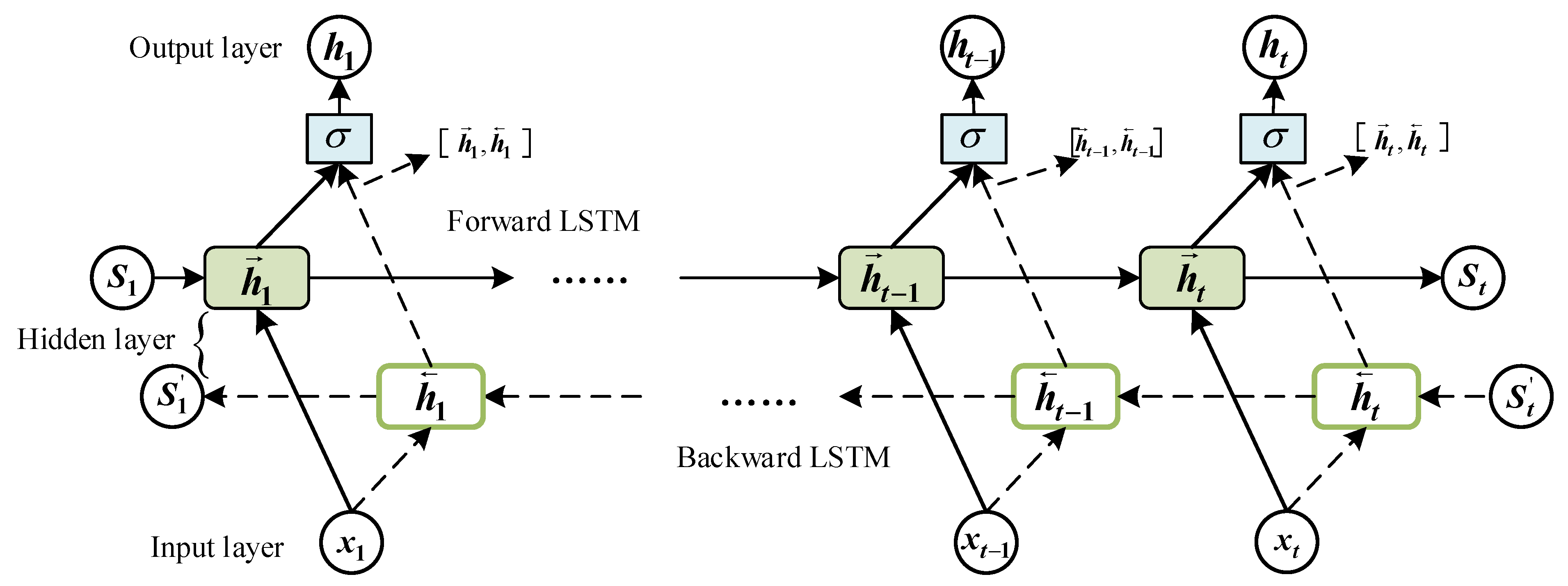
2.2.2. Bi-LSTM-Attention

In general data processing of the traditional LSTM networks, the model only processes the previous data and ignores future information. The bidirectional LSTM (Bi-LSTM) includes two LSTM modules with a forward direction and a backward direction. Both previous and later information are stored for the time series data processing at the current time. Bi-LSTM can overcome the limitations of LSTM cells that only process the previous information as opposed to using both the previous and the later ones.

The attention mechanism is proposed, based on the fact that human visual attention should be attracted to a part of the scene and should ignore unnecessary information, which is different from the idea of global attention. The attention mechanism addresses focusing on the significant region of the scene rather than on global computation. As a result, the critical part of the scene should be assigned a greater weight to address the important information. Therefore, the Bi-LSTM model can be optimized using an attention mechanism.

In this research, an attention block, which can choose the critical part of the data sequence from the global information, was adopted for Bi-LSTM. Based on the influence on the TBM advance rate prediction result, the features generated by the Bi-LSTM were assigned the corresponding weights, i.e., the attention values of the features. Therefore, the effective generated features by the Bi-LSTM layer were addressed. The attention block could create the corresponding weights automatically, and the output of the attention block is shown in Equation (6).

$${\omega }_i={\displaystyle \sum _{j=1}^n{\alpha }_{ij}{l}_j}$$

(6)

The variable l_j denotes the global features, α_ij denotes the weights of the features generated by the attention block, ω_i is the output. Attention mechanism includes soft attention and hard attention. Hard attention means selecting the concerned area as input data to decrease the training cost. However, hard attention is not suitable for time series-related problems. Moreover, hard attention makes Bi-LSTM training non-differentiable, which leads to the difficulty of training increasing sharply. The input features generated by soft attention weights focus on specific areas. The training process using soft attention is differentiable, and the end-to-end network structure can be adopted. As a result, soft attention was employed. The schematic representation of Bi-LSTM is shown in Figure 3.

2.3. Normalization and Model Evaluation Metrics

Before training, the data normalization was adopted to scale the values of the data into [0, 1], as given by:

$$x_n=\frac{x-x_{min}}{x_{max}-x_{min}}$$

(7)

where x is raw data and x_n is the normalized data; x_max and x_min are the maximum and minimum data of the sequence, respectively.

The model was established using the training data and evaluated using the test data. Reverse normalization was also applied to process the prediction result. The reverse normalization process is given by:

$$y=y_n\left(y_{max}-y_{min}\right)+y_{min}$$

(8)

where y is the real prediction result and y_n is the result with normalization; y_max and y_min are the maximum and minimum prediction values of the sequence, respectively.

In this research, three model evaluation metrics, i.e., Root Mean Square Error (RMSE), Mean Absolute Error (MAE), and R-square (R²), were adopted to evaluate the model. The three model metrics are shown in Equations (9)–(11).

$$\mathrm{RMSE}=\sqrt{\frac{1}{n}{\displaystyle \sum _{i=1}^n{\left(y_i-{\stackrel{⌢}{y}}_i\right)}^2}}$$

(9)

$$\mathrm{MAE}=\frac{1}{n}{\displaystyle \sum _{i=1}^n\left|y_i-{\stackrel{⌢}{y}}_i\right|}$$

(10)

$${\mathrm{R}}^2=1-\frac{{\displaystyle \sum _{i=1}^n{\left(y_i-{\stackrel{⌢}{y}}_i\right)}^2}}{{\displaystyle \sum _{i=1}^n{\left(y_i-{\overline{y}}_i\right)}^2}}$$

(11)

where y_i is the prediction result, ${\stackrel{⌢}{y}}_i$ is the ground truth, ${\overline{y}}_i$ is the mean value of output data. According to these equations, when RMSE and MAE are lower, and R² is higher, the prediction accuracy is higher.

3. Modeling and Results

3.1. Engineering Project Review

The TBM application engineering project was a subway construction project in Chengdu, China. The length of the subway tunnel was 43.186 km. There were 12 stations on the subway line. The maximum and minimum distances between the stations were 5.84 km and 1.46 km, respectively. The mean distance between adjacent stations was 3.58 km. The studied construction section was 4 km, and TBM was adopted for the whole section. The strata of the construction site were mainly comprised of medium-weathered sandstone and mudstone. The profile of the geological section is shown in Figure 4, indicating that the geological conditions are not complex and are easy and convenient for TMB construction.

The TBM operation data is recorded per second. The monitoring data contain 527 TBM operational parameters besides the ID and date. The TBM operational parameters include advance rate, cutter head torque, cutter head thrust, penetration, rotational speed, etc. For the study section, the monitored data of TBM operation is more than 20 GB, which is more than enough for training deep learning models.

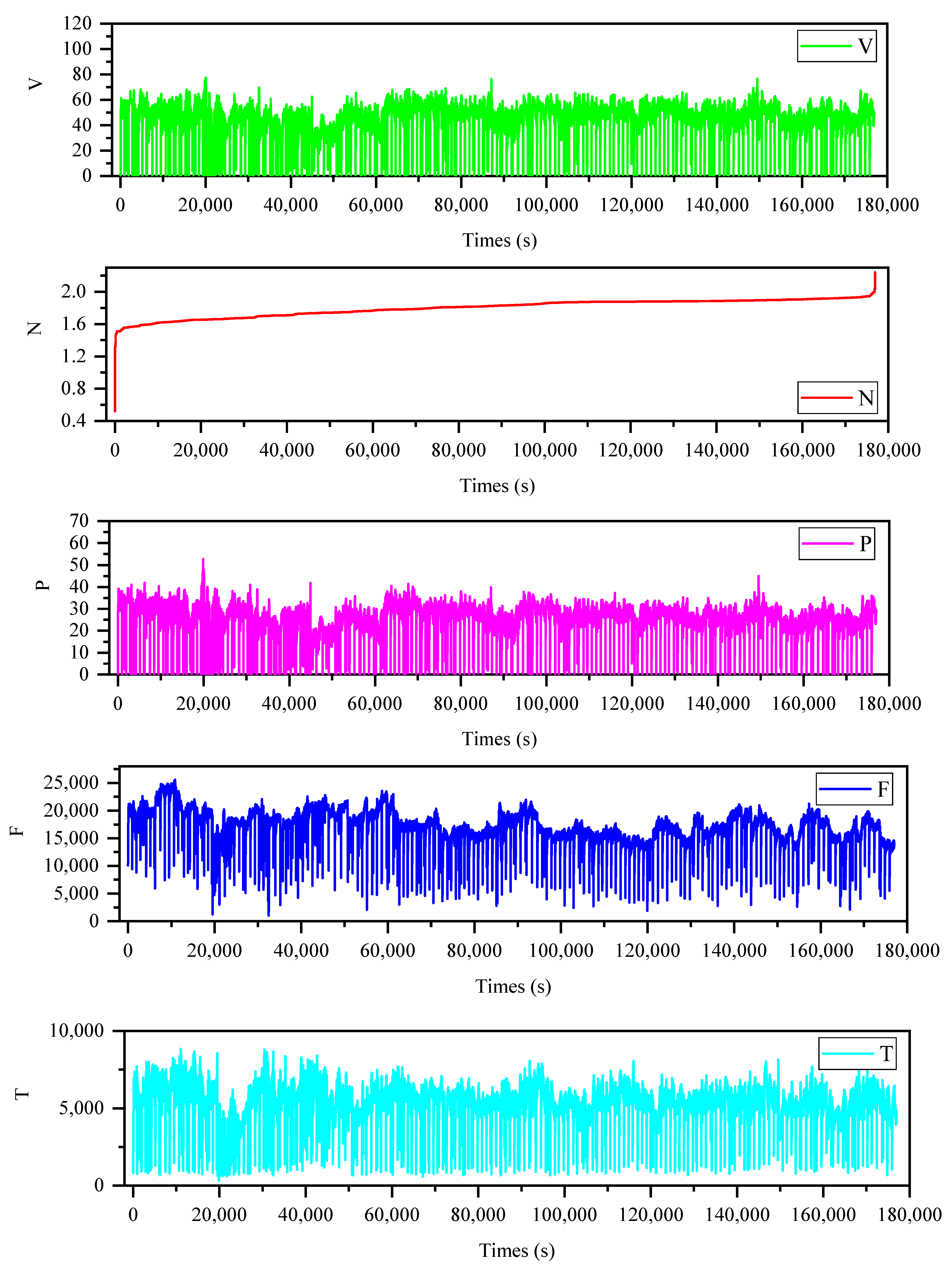
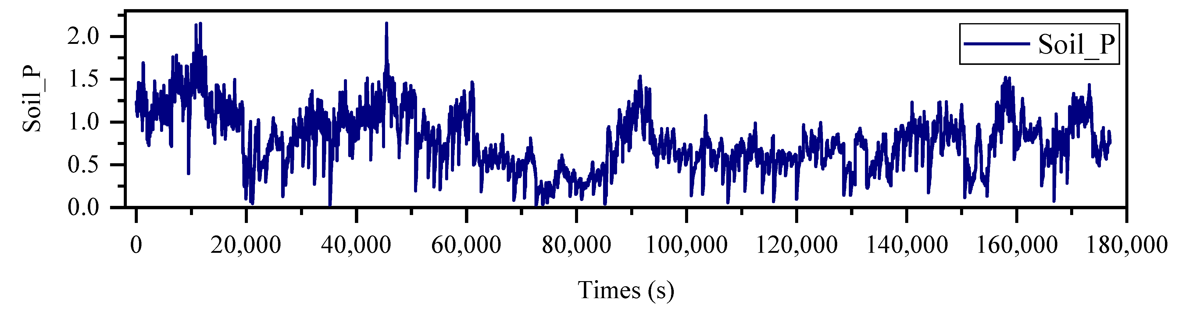
3.2. Data Profile and Preprocessing

Limited by the length of the clamp cylinder either side of the TBM, the TBM continues working through the interaction of the bracket boots, gripper, and thrusting clamp cylinder. Meanwhile, the TBM should stop working to adjust working conditions or for repairs after a working cycle. The period may last for several hours or days. The advancing-regripping state will repeat in the whole TBM working process. The monitored data should include multiple working cycles and intervals in the data sequence, as shown in Figure 5. Therefore, the working periods between the TBM working cycles should be cut off when the TBM performance analysis is carried out. Only the monitored data during the working cycles are effective for TBM performance prediction.

In a working cycle of TBM construction, there are four stages for the whole process, i.e., (I) free rotation, (II) starting stage, (III) stable operation stage, (IV) stopping stage. The specific definitions are described in [32]. The starting stage and stable operation stage are the two stages in which TMB is working. The free rotation stages are short and should be ignored in TBM performance prediction because the stages are not stable for the working state.

In this research, the monitored construction data from Day 1 to Day 27, with a total of 176,959 records, were applied. The construction section was between 98 + 901 and 99 + 045, and the strata were mainly medium-weathered sandstone, as shown in Figure 6. The data distribution of date and position is shown in

Table 1. TBM monitored data distribution for date and chainage.

Date	Chainage	Data Number
Day 1	98 + 901–98 + 905	3985
Day 2	98 + 905–98 + 908	4466
Day 3	98 + 908–98 + 918	11,095
Day 9	98 + 918–98 + 918	553
Day 10	98 + 918–98 + 918	353
Day 11	98 + 918–98 + 918	305
Day 12	98 + 918–98 + 919	345
Day 17	98 + 919–98 + 923	6014
Day 18	98 + 923–98 + 932	12,135
Day 19	98 + 923–98 + 940	11,487
Day 20	98 + 940–98 + 952	13,845
Day 21	98 + 952–98 + 964	14,169
Day 22	98 + 964–98 + 979	17,936
Day 23	98 + 979–98 + 995	19,106
Day 24	98 + 995–99 + 002	8744
Day 25	99 + 002–99 + 012	11,650
Day 26	99 + 012–99 + 022	12,286
Day 27	99 + 022–99 + 033	13,753
Day 28	99 + 033–99 + 045	14,732
Total	-	176,959

.

Some cases, such as operational mistakes, machine vibration, equipment error, and complex geological conditions, should negatively influence the data monitoring of TBM operation. Data monitoring errors may occur in the data recording process. As a result, it is necessary to remove the error from the monitoring data. In the process of TBM construction data recording, the common error is that the parameter values change sharply in a very short time. The errors often appear at the end of the working cycle and should be removed or replaced by the value of the previous recorded data. In a practical working cycle, it is impossible for the mechanical parameters to change in one or two seconds. However, the unstable working state leads to data recording errors. For example, Figure 7 shows the thrust (F) data in a working cycle of the TBM construction. At the end of the working cycle, the thrust changes to 0 from about 20,000 KN. The recorded data in red circle is regarded as an error, which is not beneficial for TBM performance analysis.

The advance rate is an important index in the TBM working process. It should be set first before the working cycle begins. The high-dimension non-linear relationship between the monitored data and the advance rate should be established. The monitored data includes the rotation speed of the cutter head (N), thrust (F), torque (T), penetration rate (P), and chamber earth pressure (Soil_P). The data structure is shown in

Table 2. Data structure.

Advance Rate (V)	N	F	T	P	Soil_P
0.146484	2.037544	2,829.455	1,279.006	0.071893	0.646701
2.270325	2.030816	2,895.904	1,147.540	1.117937	0.641276
2.270325	2.034939	2,943.162	1,080.693	1.115672	0.666884
2.197357	2.033203	25,555.990	3,005.447	1,040.585	1.080737
2.197357	2.036675	3,047.997	1,029.444	1.078894	0.710067
1.684570	2.032335	3,088.011	1,009.390	0.828884	0.735460
…	…	…	…	…	…

.

Table 3. Data application profile.

Operation Parameters	Max	Min	Medium	Unit
Advance rate (V)	112.353	0.073	46.451	mm/min
Rotation speed of cutter head (N)	2.245	0.510	1.800	rpm
Penetration rate (P)	120.977	0.037	25.889	mm/r
Thrust (F) Torque (T)	25,555.99	1,041.287	16,995.810	kN
	8,834.944	311.953	5,275.055	kN·m
Chamber earth pressure (Soil_P)	2.155	0.030	0.772	bar

and Figure 8 shows the specific variable information and distributions during the monitoring period. Table 3 shows the maximum, minimum, and medium values of the monitored data. It also shows the unit of the different types of parameters. Figure 6 shows the distributions of the different parameters. The six parameters are approximately normally distributed. It also shows the mean values and the standard deviations. The manual control of the advance rate is determined by the parameters. As a result, the advance rate should commensurate with other parameters during operation.

3.3. Model Establishment and Evaluation

In the research, the dataset was split into training data and test data. The TBM construction monitoring data of Day 27 was set as the test data. The number of test data points was 14,732, which was the last 14,732 number in the data sequence. The applied data is shown in Figure 9. All data sequences were split into training and test data.

The model structure included 64 LSTM units. It was composed of an input layer, a convolutional layer, a Bi-LSTM layer, two dropout layers, two dense layers, and two attention layers. The convolutional layer contained 448 parameters, the Bi-LSTM layer contained 66,048 parameters, and the two dense layers included 16,512 and 1025 parameters, respectively. The total number of training parameters was 84,033. Adam optimizer was adopted in model training. The MSE was selected as the loss function.

This research focused on the performance of the deep model regarding the massive amount of monitored data. Generally, more data means higher performance for deep learning models. However, because the LSTM-related models are time-dependent, it is crucial to determine the suitable data size for advance rate prediction. The data from Day 1 to Day 27 is applied, which was responding to the construction section of 98 + 901 to 99 + 045. The excavation distance was 144 m in total. To discuss the influences of the data sequence length on the model’s performance, different sizes of monitored data were applied to train the model. The five schemes are shown in

Table 4. The data profile of the five models.

Model Schemes	Date	Section	Training Data Number	Training Time (s)
1	Day 1–Day 27	98 + 901–99 + 033	162,227	4360
2	Day 20–Day 27	98 + 940–99 + 033	111,489	2994
3	Day 24–Day 27	98 + 995–99 + 033	46,433	1248
4	Day 26–Day 27	99 + 012–99 + 033	26,039	642
5	Day 27	99 + 022–99 + 033	13,753	396

.

The model was established using the Tensorflow and Keras framework. The CPU and GPU were Intel^® Core™ i9-10900K and NVIDIA Geofroce 3060 with 12G memory, respectively. The number of units was 64. In the training process of the five models, the epoch was set to 100. In one epoch, all the training data were trained once. The model loss value should decrease with the training steps. Figure 10 shows the loss change in the training process for the five models.

In Figure 10, it can be seen that the loss values converge to a small value in the training process. In Scheme 1, the loss value converges to about 3.50. In Schemes 2–4, the loss values converge to about 7.00–7.50. It shows that the five models are stable. However, the five models should be tested on the monitored data of Dec 15th.

The five models were evaluated using both the training data and the test data. The RMSE, MAE, and R² were adopted to evaluate the five models. The monitored TBM advance rate and the predicted values with time are shown in Figure 10. Because the data are massive, only the comparison of the test data and the predicted values are shown. The comparison of the model’s performances on the training and test data are shown in

Table 5. Performance of the five models.

Models	Data type	RMSE	MAE	R2
Scheme 1	Training	7.120	2.326	0.569
	Test	6.829	2.364	0.443
Scheme 2	Training	3.870	1.563	0.845
	Test	3.811	1.588	0.826
Scheme 3	Training	1.606	1.196	0.926
	Test	1.665	1.130	0.920
Scheme 4	Training	1.463	1.028	0.960
	Test	1.657	1.044	0.955
Scheme 5	Training	1.534	1.128	0.948
	Test	1.764	1.103	0.945

. The comparison of the monitored advance rate and the predicted values are shown in Figure 11.

In Figure 11, it can be seen that the models of Schemes 3–5 perform well. It denotes that unrelated data cannot promote the model performance. Meanwhile, for the deep learning models, the data size and the time should both be considered in the model establishment. In Scheme 1, although the data size is much bigger than that of other schemes, the evaluation results are worse than the others. The data number from Day 9 to Day 12 is 300 to 600. It denotes that the TBM is operated for 5–10 min. During this period, the TBM may be in a repair state. The data of the period should be ignored. In Schemes 3–5, the model of Scheme 4 outperforms the others. The construction data from Day 26 to Day 27 are set as the training data. The training data number is 26,039. In Scheme 2, the training data number is 46,433, while the model evaluation performance is worse than that of the models in Schemes 3–5. It denotes that the influence of time should be considered in data selection. Moreover, Figure 11 shows that the big prediction errors appear at the beginning of the working cycles. The result denotes that the working state of the TBM in the starting stage is still not stable and the errors increase when the TBM working state is not stable.

The predicted and monitored advance rate in the five schemes have been compared in Figure 12. y_predicted denotes the predicted advance rate; y_monitored denotes the monitored advance rate. It shows the R² distribution of the five models, indicating that the model of Scheme 4 is the best.

The R² values of the TBM advance rate are 0.443, 0.845, 0.920, 0.955 and 0.945, respectively. The different errors are given in different colors. Red means that the error is larger than 40. Yellow means that the error is in the range of (20, 40). Light blue means that the error is in the range of (10, 20). Blue means that the error is in the range of (0, 10). In Figure 11, it can be seen that the advance rate of the TBM is more than 30 mm/min. In most of the time, the advance rate is 40–50 mm/min in the working cycles. In other words, the advance rate values of 0–30 mm/min are in the starting stage. In the starting period, the TBM working state is not stable, and it negatively influences the prediction of the advance rate. As a result, the error increases when the advance rate is in the range of (0, 30). Especially when the advance rate is lower than 5 mm/min, the error is in the range of (40, 60). These results also denote that the unstable working state of the TBM negatively influences the prediction of advance rate.

A comparison of the proposed method and the traditional machine learning methods was made, including the support vector machine (SVM), random forest (RF), linear regression (LR), multilayer perceptron (MLP), and K-nearest neighbors (KNN). The scikit-learn was applied to build the models, and the parameters were chosen by the grid searching method. The results are shown in

Table 6. Comparison with the traditional machine learning models.

Data Type	RMSE	MAE	R2
SVM	3.381	3.111	0.901
RF	1.920	1.823	0.951
LR	4.196	3.949	0.845
MLP	2.252	1.799	0.939
KNN	6.513	5.154	0.492
CNN-Bi-LSTM-Attention	1.657	1.044	0.955

, and prove that the proposed method is effective for TBM advance rate prediction.

According to Table 6, the proposed model, i.e., CNN-Bi-LSTM-Attention, has the best performance of all models. KNN is an unsupervised algorithm, where only the Euler distances between samples are utilized; thus, it is difficult to achieve a good performance in such a complex task. It is also hard to catch the non-linear information of the data with LR, a classical linear model. Therefore, the R² values of KNN and LR are less than 0.90. The R² values of SVM, RF, and MLP are larger than 0.90, while they are still worse than the proposed model. The result shows that the proposed model can obtain effective information and realize an accurate prediction. Some pieces of research also support the result. Wang et al. [44] compared LSTM, RF, SVM, and DFN, and the result supports the above conclusion. Mokhtari and Mooney [45] established an SVM model with R² from 0.88 to 0.95. Fu et al. [46] employed a neural network optimized by genetic algorithm to predict advance rate, with an R² of 0.92. The result denotes that there are limitations of the shallow models in big data learning. Other researchers also applied RNN models in TBM parameter analysis. Gao et al. [36] applied RNN, LSTM, and GRU to analyze the monitored parameters, and the models achieved a high performance for torque, advance rate, and thrust prediction. Liu et al. [40] adopted LSTM and TBM real-time data to realize the tunnel lithology prediction with an accuracy of 96%. Gao et al. [41] applied an LSTM-based model to train the model using the machine parameters, rock mass parameters, and geological survey data. The result showed that the model is better than the RNN-based models as well as the autoregressive integrated moving average with explanation variables (ARIMAX) model. The data monitoring frequency is 1 Hz in TBM construction. LSTM-based models are suitable for the very large amount of monitored TBM data according to the references. The simulation result based on the subway construction data proves the conclusion. In future research, the robustness should be verified by testing the proposed model using further TBM construction data and other traditional methods.

4. Discussion

In this research, CNN-Bi-LSTM-Attention is proposed to predict the TBM advance rate. The five data sequences with different sizes were applied to build the TBM advance rate prediction model. The five models were compared, and the best training data sequence size was determined. The proposed model training time was about 400–700 s. The R² of the proposed model could reach 0.955. The result denotes that the model could be used to predict the TBM advance rate. Meanwhile, training time is available in engineering.

The limitations of the proposed model lie in a type of preference during prediction. Figure 11 shows that advance rate data between 0 and 30 mm/min was much less than that of the advance rate between 30 and 70 mm/min. As a result, the performance of the two data sequences was different. Even for Schemes 4 and 5, it denotes that the fitting of performance data with the advance rate in [0, 30) was worse than that with the advance rate in [30, 70). The result denotes that big data is necessary for the proposed method. Meanwhile, according to the result of Schemes 1, 2, and 3, the data in an unstable construction state negatively affects the model performance. In other words, it is necessary to apply clean and big data to train the proposed model.

Moreover, the proposed model could be utilized in other research studies. However, the data number should be sufficient for model training. In the research, the model in Scheme 4 with 26,039 data was the best one. The performance of the model in Scheme 5 with 13,753 data decreased. The result highlights the importance of data amount. If the proposed method is applied to another construction, clean and enough data are required.

5. Conclusions

In tunnel construction using TBM, big data is always applied in parameter prediction. However, how long the data sequence must be to be regarded as big data, and what method to choose, are the two problems in engineering projects. In this research, the effectiveness of data length is discussed, and a deep learning model is proposed for TBM monitored data analysis. LSTM-based models have been applied widely in engineering data analysis recently, and it proves that the model is effective for prediction. As a result, the deep learning model based on the CNN architecture, bidirectional Long Short-Term Memory module, and attention mechanism can be adopted to predict the TBM advance rate. RMSE, MAE, and R² were adopted to evaluate the model. The different sizes of the data sequence were applied to establish the models to verify that the data amount and data periods were both effective for the TBM advance rate. Through the comparison of the predicted values and the monitored values of the advance rate, it can be seen that the data in the starting stage cannot reflect the working state of the TBM, which may lead to prediction failure for the advance rate.

The results show that data quality is important in TBM advance rate prediction. The data in an unstable operation state is detrimental to the prediction performance. In Figure 12, it is clear that the predictions of the advance rate near 0 are very poor. The data period relates to the starting or stopping stage of TBM construction. The LSTM-based model cannot capture the information from the unstable construction state. This is because these states are too noisy, and they significantly affect the model’s performance. The results also showed that data amount is significant for TBM advance rate prediction. In Figure 12, it is clear that the prediction performance of the advance rate [0, 30) is worse than that of the advance rate [30, 70). The reason is that deep learning is a data-hungry technique. Because the data of [0, 30) are much less than the data of [30, 70), it is difficult for the model to reach a very high accuracy in this range. The proposed model outperforms all the models in the comparison with traditional machine learning methods. The results denote that it is suitable for the time-dependent data sequence because of the LSTM units. They are capable of extracting the time features to make predictions on advance rate with high accuracy.

In summary, this study showed the advantages of deep learning in the automatic analysis of the performance of TBM, and the proposed method is expected to be an auxiliary method for TBM operation, by providing an intelligent method for controlling advance rate. In the research, the model was only verified on the data from the subway construction. The rock mass is mainly composited of sandstone, which belongs to soft rock. In the future, the model should be tested on more data, especially using data from hard rock operations.

References

1. Yang, H.; Liu, X.; Song, K. A novel gradient boosting regression tree technique optimized by improved sparrow search algorithm for predicting TBM penetration rate. Arab. J. Geosci. 2022, 15, 1–15. [Google Scholar] [CrossRef]
2. Yang, H.; Wang, H.; Zhou, X. Analysis on the rock–cutter interaction mechanism during the TBM tunneling process. Rock Mech. Rock Eng. 2016, 49, 1073–1090. [Google Scholar] [CrossRef]
3. Zeng, J.; Roy, B.; Kumar, D.; Mohammed, A.S.; Armaghani, D.J.; Zhou, J.; Mohamad, E.T. Proposing several hybrid PSO-extreme learning machine techniques to predict TBM performance. Eng. Comput. 2021, 1–17. [Google Scholar] [CrossRef]
4. Barton, N.R. TBM Tunnelling in Jointed and Faulted Rock; CRC Press: Boca Raton, FL, USA, 2000. [Google Scholar]
5. Blindheim, O.T. Boreability Predictions for Tunneling; The Norwegian Institute of Technology: Trondheim, Norway, 1979. [Google Scholar]
6. Bruland, A. Hard Rock Tunnel Boring; Fakultet for Ingeniørvitenskap og Teknologi: Trondheim, Norway, 2000. [Google Scholar]
7. Sapigni, M.; Berti, M.; Bethaz, E.; Busillo, A.; Cardonee, G. TBM performance estimation using rock mass classifications. Int. J. Rock Mech. Min. Sci. 2002, 39, 771–788. [Google Scholar] [CrossRef]
8. Kahraman, S.; Bilgin, N.; Feridunoglu, C. Dominant rock properties affecting the penetration rate of percussive drills. Int. J. Rock Mech. Min. Sci. 2003, 40, 711–723. [Google Scholar] [CrossRef]
9. Hassanpour, J.; Rostami, J.; Khamehchiyan, M.; Bruland, A. Developing new equations for TBM performance prediction in carbonate-argillaceous rocks: A case history of Nowsood water conveyance tunnel. Geomech. Geoengin. Int. J. 2009, 4, 287–297. [Google Scholar] [CrossRef]
10. Kasper, T.; Meschke, G. On the influence of face pressure, grouting pressure and TBM design in soft ground tunnelling. Tunn. Undergr. Space Technol. 2006, 21, 160–171. [Google Scholar] [CrossRef]
11. Gong, Q.M.; Zhao, J. Development of a rock mass characteristics model for TBM penetration rate prediction. Int. J. Rock Mech. Min. Sci. 2009, 46, 8–18. [Google Scholar] [CrossRef]
12. Li, X.; Li, H.; Liu, Y.; Zhou, Q.; Xia, X. Numerical simulation of rock fragmentation mechanisms subject to wedge penetration for TBMs. Tunn. Undergr. Space Technol. 2016, 53, 96–108. [Google Scholar] [CrossRef]
13. Zhong, G.; Wang, L.-N.; Ling, X.; Dong, J. An overview on data representation learning: From traditional feature learning to recent deep learning. J. Financ. Data Sci. 2016, 2, 265–278. [Google Scholar] [CrossRef]
14. Sun, W.; Shi, M.; Zhang, C.; Zhao, J.; Song, X. Dynamic load prediction of tunnel boring machine (TBM) based on heterogeneous in-situ data. Autom. Constr. 2018, 92, 23–34. [Google Scholar] [CrossRef]
15. Mahdevari, S.; Shahriar, K.; Yagiz, S.; Shirazi, M.A. A support vector regression model for predicting tunnel boring machine penetration rates. Int. J. Rock Mech. Min. Sci. 2014, 72, 214–229. [Google Scholar] [CrossRef]
16. Zhou, J.; Qiu, Y.; Zhu, S.; Armaghani, D.J.; Li, C.; Nguyen, H.; Yagiz, S. Optimization of support vector machine through the use of metaheuristic algorithms in forecasting TBM advance rate. Eng. Appl. Artif. Intell. 2021, 97, 104015. [Google Scholar] [CrossRef]
17. Noori, A.M.; Mikaeil, R.; Mokhtarian, M.; Haghshenas, S.S.; Foroughi, M. Feasibility of intelligent models for prediction of utilization factor of TBM. Geotech. Geol. Eng. 2020, 38, 3125–3143. [Google Scholar] [CrossRef]
18. Afradi, A.; Ebrahimabadi, A.; Hallajian, T. Prediction of TBM penetration rate using fuzzy logic, particle swarm optimization and harmony search algorithm. Geotech. Geol. Eng. 2022, 40, 1513–1536. [Google Scholar] [CrossRef]
19. LeCun, Y.; Bengio, Y.; Hinton, G. Deep learning. Nature 2015, 521, 436–444. [Google Scholar] [CrossRef]
20. Goodfellow, I.; Bengio, Y.; Courville, A. Deep Learning; MIT press: Cambridge, MA, USA, 2016. [Google Scholar]
21. Bengio, Y.; Goodfellow, I.; Courville, A. Deep Learning; MIT press: Cambridge, MA, USA, 2017. [Google Scholar]
22. Tian, C.; Fei, L.; Zheng, W.; Xu, Y.; Zuo, W.; Lin, C.W. Deep learning on image denoising: An overview. Neural Netw. 2020, 131, 251–275. [Google Scholar] [CrossRef]
23. Wang, Z.; Chen, J.; Hoi, S.C.H. Deep learning for image super-resolution: A survey. IEEE Trans. Pattern Anal. Mach. Intell. 2020, 42, 3365–3387. [Google Scholar] [CrossRef]
24. Salamon, J.; Bello, J.P. Deep convolutional neural networks and data augmentation for environmental sound classification. IEEE Signal Processing Lett. 2017, 24, 279–283. [Google Scholar] [CrossRef]
25. Kim, J.; Min, K.; Jung, M.; Chi, S. Occupant behavior monitoring and emergency event detection in single-person households using deep learning-based sound recognition. Build. Environ. 2020, 181, 107092. [Google Scholar] [CrossRef]
26. Majumder, N.; Poria, S.; Gelbukh, A.; Erik, C. Deep learning-based document modeling for personality detection from text. IEEE Intell. Syst. 2017, 32, 74–79. [Google Scholar] [CrossRef]
27. Chatterjee, A.; Gupta, U.; Chinnakotla, M.K.; Srikanth, R.; Galley, M.; Agrawal, P. Understanding emotions in text using deep learning and big data. Comput. Hum. Behav. 2017, 93, 309–317. [Google Scholar] [CrossRef]
28. Rumelhart, D.E.; Hinton, G.E.; Williams, R.J. Learning representations by back-propagating errors. Nature 1986, 323, 533–536. [Google Scholar] [CrossRef]
29. Lecun, Y.; Bottou, L.; Bengio, Y.; Haffner, P. Gradient-based learning applied to document recognition. Proc. IEEE 1998, 86, 2278–2324. [Google Scholar] [CrossRef]
30. Hinton, G.E.; Osindero, S.; Teh, Y.W. A fast learning algorithm for deep belief nets. Neural Comput. 2006, 18, 1527–1554. [Google Scholar] [CrossRef]
31. Hinton, G.E.; Salakhutdinov, R.R. Reducing the dimensionality of data with neural networks. Science 2006, 313, 504–507. [Google Scholar] [CrossRef]
32. Ren, Q.B.; Li, M.C.; Li, H.; Shen, Y. A novel deep learning prediction model for concrete dam displacements using interpretable mixed attention mechanism. Adv. Eng. Inform. 2021, 50, 101407. [Google Scholar] [CrossRef]
33. Li, M.C.; Li, M.H.; Ren, Q.B.; Li, H.; Song, L.G. DRLSTM: A dual-stage deep learning approach driven by raw monitoring data for dam displacement prediction. Adv. Eng. Inform. 2022, 51, 101510. [Google Scholar] [CrossRef]
34. Bai, S.; Li, M.C.; Lu, Q.R.; Tian, H.J.; Qin, L. Global Time Optimization Method for Dredging Construction Cycles of Trailing Suction Hopper Dredger Based on Grey System Model. J. Constr. Eng. Manag. 2022, 148, 04021198. [Google Scholar] [CrossRef]
35. Zhang, P.; Yin, Z.Y.; Zheng, Y.Y.; Gao, F.P. A LSTM surrogate modelling approach for caisson foundations. Ocean. Eng. 2020, 204, 107263. [Google Scholar] [CrossRef]
36. Gao, X.; Shi, M.; Song, X.; Zhang, C.; Zhang, H. Recurrent neural networks for real-time prediction of TBM operating parameters. Autom. Constr. 2019, 98, 225–235. [Google Scholar] [CrossRef]
37. Feng, S.; Chen, Z.; Luo, H.; Wang, S.; Zhao, Y.; Liu, L.; Ling, D.; Jing, L. Tunnel boring machines (TBM) performance prediction: A case study using big data and deep learning. Tunn. Undergr. Space Technol. 2021, 110, 103636. [Google Scholar] [CrossRef]
38. Chen, Z.; Zhang, Y.; Li, J.; Li, X.; Jing, L. Diagnosing tunnel collapse sections based on TBM tunneling big data and deep learning: A case study on the Yinsong Project, China. Tunn. Undergr. Space Technol. 2021, 108, 103700. [Google Scholar] [CrossRef]
39. Graves, A. Long Short-Term Memory. Supervised Sequence Labelling with Recurrent Neural Networks; Springer: Berlin/Heidelberg, Germany, 2012; pp. 37–45. [Google Scholar] [CrossRef]
40. Liu, Z.; Li, L.; Fang, X.; Qi, W.; Shen, J.; Zhou, H.; Zhang, Y. Hard-rock tunnel lithology prediction with TBM construction big data using a global-attention-mechanism-based LSTM network. Autom. Constr. 2021, 125, 103647. [Google Scholar] [CrossRef]
41. Gao, B.; Wang, R.; Lin, C.; Guo, X.; Liu, B.; Zhang, W. TBM penetration rate prediction based on the long short-term memory neural network. Undergr. Space 2021, 6, 718–731. [Google Scholar] [CrossRef]
42. Fu, X.; Zhang, L. Spatio-temporal feature fusion for real-time prediction of TBM operating parameters: A deep learning approach. Autom. Constr. 2021, 132, 103937. [Google Scholar] [CrossRef]
43. Li, L.; Liu, Z.; Zhou, H.; Zhang, J.; Shen, W.; Shao, J. Prediction of TBM cutterhead speed and penetration rate for high-efficiency excavation of hard rock tunnel using CNN-LSTM model with construction big data. Arab. J. Geosci. 2022, 15, 1–17. [Google Scholar] [CrossRef]
44. Wang, Q.; Xie, X.; Shahrour, I. Deep learning model for shield tunneling advance rate prediction in mixed ground condition considering past operations. IEEE Access 2020, 8, 215310–215326. [Google Scholar] [CrossRef]
45. Mokhtari, S.; Mooney, M.A. Predicting EPBM advance rate performance using support vector regression modeling. Tunn. Undergr. Space Technol. 2020, 104, 103520. [Google Scholar] [CrossRef]
46. Fu, X.; Gong, Q.; Wu, Y.; Zhao, Y.; Li, H. Prediction of EPB Shield Tunneling Advance Rate in Mixed Ground Condition Using Optimized BPNN Model. Appl. Sci. 2022, 12, 5485. [Google Scholar] [CrossRef]
Figure 1. Overall framework of CNN-Bi-LSTM-Attention model.
Buildings 12 01567 g001
Figure 2. The structure of an LSTM block.
Buildings 12 01567 g002
Figure 3. Schematic representation of Bi-LSTM.
Buildings 12 01567 g003
Figure 4. Geological conditions of the TBM construction section.
Buildings 12 01567 g004
Figure 5. Working cycles and intervals in TBM construction monitored data.
Buildings 12 01567 g005
Figure 6. The different stages of TBM working cycle.
Buildings 12 01567 g006
Figure 7. Error recording in TBM working cycle.
Buildings 12 01567 g007
Figure 8. Distribution of the TBM construction parameters. (a) V (b) N (c) P (d) F (e) T (f) Soil_P.
Buildings 12 01567 g008
Figure 9. The training and test monitored data of the TBM construction.
Buildings 12 01567 g009aBuildings 12 01567 g009b
Figure 10. Loss changes in the training processes of all the training schemes.
Buildings 12 01567 g010
Figure 11. The evaluation of the models in the five schemes.
Buildings 12 01567 g011aBuildings 12 01567 g011b
Figure 12. Comparison of the advance rate monitored and predicted.
Buildings 12 01567 g012aBuildings 12 01567 g012b