The Reduced-Degree-of-Freedom Model for Seismic Analysis of Predominantly Plan-Symmetric Reinforced Concrete Wall–Frame Building

Abstract

A reduced-degree-of-freedom (RDOF) model for seismic analysis of predominantly plan-symmetric reinforced concrete (RC) wall–frame buildings is introduced. The RDOF model of the wall–frame building consists of elastic beam–column elements with concentrated plasticity used for simulating cantilever walls and predominantly plan-symmetric RC frame buildings that are represented by the improved fish-bone (IFB) model. In this paper, the capability of the RDOF model is demonstrated for two frame buildings and two wall–frame buildings. The RDOF models were defined directly from the building information model. This is an advantage of RDOF models with respect to single-degree-of-freedom (SDOF) models, while the computational robustness of the RDOF models also makes them attractive for the seismic analysis of building stock. The imposed cyclic displacement analyses conducted for the investigated buildings proved that the condensation of the degrees of freedom for RDOF models was appropriate. Consequently, only minor differences were observed for maximum storey drift IDA curves, maximum storey acceleration IDA curves, and seismic fragility functions for different limit states. However, development is needed to make RDOF models appropriate for preliminary seismic performance assessment of plan-irregular buildings.

1. Introduction

The simulation of seismic response of buildings is often performed by utilizing conventional multiple-degree-of-freedom (MDOF) models (e.g., [1,2,3]). By increasing the number of elements, the robustness and time-efficiency of such a structural model decreases. Thus, the MDOF models are robust and time-efficient only to a certain number of structural elements. This issue is not so evident if the objective is to estimate the seismic response of a single building. It becomes especially relevant when the seismic response analysis is performed for a building portfolio rather than for a single building. Consequently, structural models have to be simplified for seismic analysis of building stock due to low computational robustness and time inefficiency and the lack of building stock input data. The simplest alternative to the conventional MDOF model is the single-degree-of-freedom (SDOF) model, which can be most precisely defined based on the pushover analysis of the MDOF model (e.g., [4,5,6]). However, SDOF models have certain limitations. Their use is still limited to buildings with an insignificant effect of higher modes. However, more challenging is to define the SDOF model without performing a pushover analysis [7] and even to transform the SDOF model results to the engineering demand parameters (EDPs) at the building level [6].

To address the issue of low computational robustness and time inefficiency, simplified MDOF models have been introduced in addition to SDOF models. Simplified MDOF models represent the intermediate stage between MDOF and SDOF models. For the analysis of frame buildings, several simplified MDOF models for the seismic response analysis were proposed, for example, variants of generic-frame (GF) models and fish-bone (FB) models [8,9,10,11,12,13]. The fish-bone (FB) model was introduced by Ogawa et al. [8], while Nakashima et al. [9] proposed the generic frame (GF) model. In both cases, the simplified models were used for the seismic response analysis of steel moment frames [14]. Further on, several different variants and modifications of the GF and FB model were proposed, which improved the capability of the simplified models for simulating the seismic response of the building structures [10,11,12,13,14,15,16,17,18]. Firstly, the authors developed simplified MDOF models to be an alternative to MDOF models used for seismic performance assessment of a single building. However, today, simplified models are used for seismic performance of building stock and complex seismic analysis involving thousands of simulations. Thus, several other types of simplified models were developed. For example, the continuous model consists of a flexural and shear cantilever beam connected by axially rigid links [19,20,21]. This type of model was used for seismic analysis of multi-storey buildings with different structural systems. Although all simplified MDOF models have several limitations, including the introduced RDOF model, they can be defined directly based on the building data, which is much more challenging in the case of the SDOF model. This advantage is quite important if the objective is a seismic analysis of building stock.

It was shown before that the simplified MDOF models could provide quite precise results of the seismic response of older and contemporary reinforced concrete (RC) frame buildings. An extensive parametric study involving the simulation of seismic response of different frame buildings was also presented recently by Jamšek and Dolšek [13]. It was proven that the improved fish-bone (IFB) model could provide sufficiently accurate engineering demand parameters (EDPs) of pseudo-dynamically tested frame buildings and can also be successfully used for seismic fragility and risk analysis. The IFB model accounts for the importance of structural elements and the effect of potential redistribution of seismic demands, which makes it possible to be applied to older and contemporary predominantly plan-symmetric reinforced concrete frame buildings.

This paper attempts to extend the IFB model to a RDOF model, which is computationally time-efficient, robust, and accurate for seismic analysis of different structural systems of reinforced concrete buildings. The idea is based on the pseudo-three-dimensional nonlinear mathematical model proposed by Kilar and Fajfar [22,23], where different 2D macro-elements were defined for substructures (e.g., frames, walls, coupled walls) connected by rigid diaphragms at the storey level. The RDOF model presented in this study consists of the IFB model (Figure 1a) used to simulate predominantly plan-symmetric frame building [13] and beam–column elements, which are used to simulate cantilever walls (Figure 1b). The elastic beam–column elements with concentrated plasticity (i.e., plastic hinges) were utilized for the simplistic presentation of cantilever walls. Therefore, the introduced RDOF models are suitable only for modelling the global response of simple wall–frame buildings with a predominantly flexural response. The study is also limited to predominantly plan-symmetric buildings. For easier notation, the simplified models are hereinafter termed as RDOF models. The IFB model is thus understood as a variant of the RDOF model used to simulate the seismic response of frame building.

Firstly, in Section 2, the concept of the RDOF model is introduced by summarizing the description of the IFB model for frame buildings and the RDOF model for simple dual wall–frame buildings. Then, in Section 3, the investigated buildings are described. Two reinforced concrete frame buildings are presented in addition to two simple dual wall–frame buildings. All the investigated buildings were taken from previous studies (e.g., [13,24]). The capabilities of the presented models (IFB and RDOF) are then demonstrated in Section 4 by comparing the base shear – storey drift relationship, IDA curves, and fragility functions from the simplified models and the conventional MDOF models. Conclusions of the study are gathered in Section 5.

2. Description of the RDOF Models

For the RDOF model’s definition, the building information model should be the same as that required for the definition of the conventional multi-degree-of-freedom (MDOF) model. In general, the information about the building structure geometry, designed or built-in material characteristics, reinforcement geometry, the gravity loads, and storey masses. Additional information can then be derived. For example, geometrical constants of the structural elements, gravity loads and corresponding loads on structural elements, and parameters of plastic hinges of the structural elements can be calculated to develop a model for structural analysis. In this study, flexural plastic hinges were defined by a tri-linear moment-rotation relationship accounting for the softening branch (e.g., [3,24]). The so-defined building information model can be used to automatically develop the MDOF models or the RDOF model.

In this study, the conventional MDOF model was used as a point of comparison. Even though each column, beam, and wall were modelled in this case, the model is still simplistic because it accounts only for flexural plastic hinges. However, if a nonductile failure mechanism could be predominant, e.g., shear failures of beams, columns, walls or joints, more detailed models should be considered, e.g., for RC walls, the MVLEM model can be considered [25]. Another alternative is an approximate modification of the nonlinear relationship of plastic hinges proposed by Celarec and Dolšek [26]. Further, it should be emphasized that RDOF models, as presented in this paper, can be applied only to predominantly plan-symmetric buildings. Additionally, the limitations of the models introduced by Nakashima et al. [9] should be considered where the models are sufficiently accurate for buildings with at least one bay frame and that building’s height is less than three times the building length.

In the following, the IFB model is first summarized by addressing the first level assumptions common to the conventional MDOF model and the second level assumptions related only to the IFB model. Finally, the RDOF model, consisting of the IFB model and the elastic beam-column element with plastic hinges, is briefly described. It makes sense to note that the parameters of plastic hinges of the IFB and RDOF models are the same as those of the MDOF model [2,24]. However, the properties of plastic hinges of the IFB model are considerably different from those of the particular columns and beams of an RC frame building [13], which is also discussed in Section 2.1.2. However, the properties of plastic hinges of the cantilever walls of the MDOF and RDOF model are the same because the structural element configuration of cantilever walls for the MDOF and RDOF model is the same.

2.1. The IFB Model for Frame Buildings

2.1.1. The First Level Assumptions Common to the Conventional MDOF Model

The first level assumptions of the IFB model are common to those considered in the definition of the MDOF model of reinforced concrete frames. Several studies [2,3,24] have concluded that the MDOF models are adequately accurate for simulating the seismic response of frame building to the near-collapse limit-state, even though they are defined with several assumptions. Masses are modelled only at the elevation of storeys. The material nonlinearity is assumed concentrated in plastic hinges of the columns and beams. Properties of plastic hinges account for flexural failure only by a predefined moment–rotation relationship according to the procedure used by Haselton et al. [2] and Dolšek [24]. Therefore, it was assumed that the plastic hinges are modelled by a tri-linear moment–rotation relationship accounting for a linear softening branch in the postcapping range (Figure 2). For the definition of the tri-linear moment–rotation relationship, only three characteristic points are needed. All three characteristic points are defined by three characteristic moments—the yield moment (${\mathrm{M}}_{\mathrm{Y}}$), maximum moment (${\mathrm{M}}_{\mathrm{M}}$), and ultimate moment (${\mathrm{M}}_{\mathrm{U}}$), while the corresponding rotations were named characteristic rotations (${\mathsf{\Theta }}_{\mathrm{Y}}$, ${\mathsf{\Theta }}_{\mathrm{M}}$, ${\mathsf{\Theta }}_{\mathrm{U}}$) (Figure 2). The characteristic moments of the moment–rotation relationship of plastic hinges are calculated by moment-curvature analysis of the columns and beams cross-section, which is based on the stress-strain relationship according to the Eurocode 2 requirements [27] and constant axial forces from gravity analysis. For calculating characteristic rotations, the point of contra-flexure at the mid-span of columns and beams was assumed [3]. Additionally, the effective beam widths were taken into account according to Eurocode 2 provisions [27]. The effective stiffness of structural elements was considered equal to half of the initial stiffness according to Eurocode 8 [28]. The shear behavior and the nonlinear behavior of beam–column joints was neglected.

2.1.2. The Second Level Assumptions Introduced for the IFB Model’s Definition

The second level assumptions are introduced only for the IFB model definition. These assumptions are additional to those common to the MDOF model. Although the IFB model [13], which is summarized in this section, introduced several improvements compared to the FB model [8,9,14], it is a subject of quite some assumption. The structural configuration of the FB or IFB model can be significantly different to the frame building. Consequently, the number of structural elements of a frame building (Figure 3a) is condensed to the configuration of structural elements of the FB or IFB model (Figure 3b). This step is the same as in the case of the original FB model [8,9]. Almost all other assumptions originate from this basic assumption, which introduces a reduction in the number of structural elements.

The height of the column of the IFB model was considered to be equal to the storey height of the frame building. Note that the columns and beams of the IFB model are hereinafter termed as IFB columns and IFB beams. The IFB columns’ moment of inertia in a given storey was calculated as the sum of moments of inertia of columns in that storey [9]. An analogous assumption was made of the cross-section areas of the IFB beams. In general, the moment of inertia of IFB beams ${\mathrm{I}}_{\mathrm{b},\mathrm{i}}^{\mathrm{F}}$ accounts for the variation of beam lengths [13], but in this study, a simplification was considered so that the ${\mathrm{I}}_{\mathrm{b},\mathrm{i}}^{\mathrm{F}}$ is equal to:

$${\mathrm{I}}_{\mathrm{b},\mathrm{i}}^{\mathrm{F}}={\displaystyle \sum }_{\mathrm{k}=1}^{\mathrm{n}}{\mathrm{I}}_{\mathrm{b},\mathrm{i},\mathrm{k}}$$

(1)

where F refers to the parameters of the IFB model, b refers to beams of either the MDOF or IFB model, i is the number of a storey, and k refers to a beam in the particular storey. ${\mathrm{I}}_{\mathrm{b},\mathrm{i}}^{\mathrm{F}}$is thus estimated as the sum of the moment of inertia of the corresponding k-th beams in i-th storey. This simplification is not necessary, but it was introduced because it was observed that it has only a minor impact on the initial stiffness of the IFB model and, consequently, on the results of the seismic analysis of reinforced concrete frame buildings. However, if the variation of beam length in the corresponding storey highly varies from beam to beam, such a simplification may not be appropriate.

The length of the IFB beam ${\mathrm{L}}_{\mathrm{b},\mathrm{i}}^{\mathrm{F}}$ (Figure 3b) was defined as one half of the average length of the beams ${\mathrm{L}}_{\mathrm{b},\mathrm{i},\mathrm{k}}$ in that storey (Figure 3a), considering that the IFB beams are restrained at the mid-span (Figure 3b). Applying gravity loads on the IFB columns and beams was considered by analogy to gravity loads on the MDOF model [24], i.e., as point loads on columns and uniformly distributed line loads on beams. A new approach was also defined for the loads on the IFB beams [13], considering the redistribution of vertical loads due to the plastic hinge on one side of the IFB beam and vertical support on the other, as presented for the 1st (i = 1) and 2nd (i = 2) storey of the IFB model in Figure 3b. The redistribution of vertical loads was considered with a new parameter used for multiplying the uniformly distributed line loads on IFB beams; thus, in the IFB column and beam joint, the appropriate level of the vertical loads is transferred. With the new parameter, an appropriate level of axial forces in the IFB column can be estimated.

The adopted tri-linear moment-rotation relationship of IFB columns and beams simulates an approximate softening of the structural element behavior, as presented in Figure 2 [2,24]. It should be noted that the IFB model and the MDOF model can be defined with different moment–rotation relationships. The IFB model’s capability and accuracy remain satisfactory, even when the moment–rotation relationship is characterized by a different model with more characteristic points [29].

A new procedure was required to define the characteristic moments of the IFB column and IFB beam, because the columns in a given storey are modelled with a single IFB column and the beams with two IFB beams. The characteristic moments of IFB columns’ plastic hinges were calculated as the sum of the character moments of the columns of the designated storey:

$${\mathrm{M}}_{\mathrm{c},\mathrm{i},\mathrm{h},\mathrm{p}}^{\mathrm{F}}={\displaystyle \sum }_{\mathrm{j}=1}^{\mathrm{m}}{\mathrm{M}}_{\mathrm{c},\mathrm{i},\mathrm{j},\mathrm{h},\mathrm{p}}$$

(2)

where c denotes an IFB column and a column of the frame building, i, j, h, p refer, respectively, to the storey, particular column in the storey, a hinge of the column and the particular characteristic moment, and ${\mathrm{M}}_{\mathrm{c},\mathrm{i},\mathrm{j},\mathrm{h},\mathrm{p}}$ is a characteristic moment of the column of a frame building. For a more straightforward representation, all the indices are presented in Figure 3. The same procedure can be applied for assessing the p-th characteristic moment of the IFB beam for the h-th hinge in the i-th storey ${\mathrm{M}}_{\mathrm{b},\mathrm{i},\mathrm{h},\mathrm{p}}^{\mathrm{F}}$ if the building was designed following the strong column – weak beam design approach:

$${\mathrm{M}}_{\mathrm{b},\mathrm{i},\mathrm{h},\mathrm{p}}^{\mathrm{F}}={\displaystyle \sum }_{\mathrm{k}=1}^{\mathrm{n}}{\mathrm{M}}_{\mathrm{b},\mathrm{i},\mathrm{k},\mathrm{h},\mathrm{p}}$$

(3)

where b denotes an IFB beam or a beam of the frame building and i,k,h,p refer, respectively, to the storey, particular beam in the storey, a hinge of the beam, and the particular characteristic moment of a given IFB beam or a beam of the frame building. ${\mathrm{M}}_{\mathrm{b},\mathrm{i},\mathrm{k},\mathrm{h},\mathrm{p}}$ refers to the characteristic moment of the beam of the frame building. However, if the building (e.g., older reinforced concrete frames) was designed without considering the concept of the strong column – weak beam, i.e., according to the capacity design approach as prescribed in Eurocode 8 provisions [29], then the characteristic moments of the IFB beams, ${\mathrm{M}}_{\mathrm{b},\mathrm{i},\mathrm{h},\mathrm{p}}^{\mathrm{F}}$, should be estimated with the reduced contribution of the beam strength as proposed by Jamšek and Dolšek [13]. If the reduction in the beam strength is not introduced in the FB model of the older reinforced concrete frames, the nonlinearity effects are fully concentrated in an FB column. However, for the MDOF models, plasticity can also be observed in the beams. Due to the concentration of the plastic mechanism in the FB column, the base shear of such an FB model can be overestimated, while the deformation capacity can be highly underestimated [13] with respect to the performance of the MDOF model. Such a performance of the FB model is the consequence of the reduction in degrees of freedom. All the beam-column joints in a storey are condensed into a single column–beam joint (Figure 3). Therefore, the equilibrium of moment demand in the beam–column joints is no longer explicitly specified at the level of beam-column joints but at the storey level. This issue was precisely investigated before [13]. It was found that the plastic mechanism of IFB models of older reinforced concrete frame buildings is significantly better than those simulated by the conventional FB model, where the IFB beams’ characteristic moments were defined with the consideration of the beam-column joints’ maximum moment equilibrium. Consequently, the base shear and deformation capacity of IFB models are better than those based on conventional FB models.

Moreover, the corresponding characteristic rotations in the IFB columns’ and beams’ plastic hinges, ${\mathsf{\Theta }}_{\mathrm{c},\mathrm{i},\mathrm{h},\mathrm{p}}^{\mathrm{F}}$ ${\mathsf{\Theta }}_{\mathrm{b},\mathrm{i},\mathrm{h},\mathrm{p}}^{\mathrm{F}}$, were defined as the weighted average of the corresponding characteristic rotations of columns ${\mathsf{\Theta }}_{\mathrm{c},\mathrm{i},\mathrm{j},\mathrm{h},\mathrm{p}}$ and beams ${\mathsf{\Theta }}_{\mathrm{b},\mathrm{i},\mathrm{k},\mathrm{h},\mathrm{p}}$, respectively. The weights were assumed to be equal to the corresponding characteristic moments to at least approximately consider that the structural elements with greater strength (e.g., yield and maximum moments) have a more considerable effect on the definition of the IFB columns’ and beams’ characteristic rotations.

$${\mathsf{\Theta }}_{\mathrm{c},\mathrm{i},\mathrm{h},\mathrm{p}}^{\mathrm{F}}=\frac{{{\displaystyle \sum }}_{\mathrm{j}=1}^{\mathrm{m}}{(\mathsf{\Theta }}_{\mathrm{c},\mathrm{i},\mathrm{j},\mathrm{h},\mathrm{p}}·{\mathrm{M}}_{\mathrm{c},\mathrm{i}, \mathrm{j},\mathrm{h},\mathrm{p}})}{{{\displaystyle \sum }}_{\mathrm{j}=1}^{\mathrm{m}}{\mathrm{M}}_{\mathrm{c},\mathrm{i},\mathrm{j},\mathrm{h},\mathrm{p}}}$$

(4)

$${\mathsf{\Theta }}_{\mathrm{b},\mathrm{i},\mathrm{h}, \mathrm{p}}^{\mathrm{F}}=\frac{{{\displaystyle \sum }}_{\mathrm{k}=1}^{\mathrm{n}}{(\mathsf{\Theta }}_{\mathrm{b},\mathrm{i},\mathrm{k},\mathrm{h},\mathrm{p}}·{\mathrm{M}}_{\mathrm{b},\mathrm{i},\mathrm{k},\mathrm{h},\mathrm{p}})}{{{\displaystyle \sum }}_{\mathrm{k}=1}^{\mathrm{n}}{\mathrm{M}}_{\mathrm{b},\mathrm{i},\mathrm{k},\mathrm{h},\mathrm{p}}}$$

(5)

2.2. The RDOF Model for the Analysis of Simple Wall–Fame Buildings

The RDOF model is a simplified extension of the IFB model with the elastic beam–column element(s) with plastic hinges, constrained at the storey level by assuming a rigid diaphragm. Such a simplified model is intended to be used for the seismic analysis of simple reinforced concrete (RC) wall–frame buildings. The structural system consists of frames and cantilever walls. In general, the RDOF model can include several IFB models and several elastic beam-column elements with plastic hinges. Consequently, the reduction in structural elements is related to the condensation of the frame elements, which can still significantly simplify the conventional MDOF models, which consist of separate elements for beams, columns, and cantilever walls. The MDOF and the RDOF model of a simple frame–wall building are presented in Figure 4.

The assumption of the rigid diaphragm at the storey level, as presented in Figure 4 for both models with axially rigid links (𝐴→∞), does not introduce significant error if the slab strength and stiffness are relatively high. The characteristics of the frame in the case of the RDOF model are those presented for the IFB model. In contrast, the cantilever wall is modelled with an elastic beam–column element with a single plastic hinge per storey just above the storey level [30]. The linear elastic model of the cantilever wall is thus defined by the geometric constants (cross-section $\mathrm{A}$, length L, moment of inertia$\mathrm{I}$) and modulus of elasticity of the material. The nonlinear effects are modelled by plastic hinges, as presented in Figure 4. The shape of the moment-rotation relationship of the plastic hinges of cantilever walls is considered the same as for the columns and beams (Figure 2). Therefore, the plastic hinges of the cantilever walls are defined with the tri-linear moment-rotation relationship, accounting for the linear postcapping behavior. Consequently, the plastic hinges of the cantilever walls of the MDOF model as well as of the RDOF model are defined with three characteristic moments, ${\mathrm{M}}_{\mathrm{w},\mathrm{i},\mathrm{p}}$ and ${\mathrm{M}}_{\mathrm{w},\mathrm{i},\mathrm{p}}^{\mathrm{R}}$, respectively, and corresponding characteristic rotations. Thus, for the major axis of the cantilever wall, the yield ${\mathrm{M}}_{\mathrm{Y}}$, maximum ${\mathrm{M}}_{\mathrm{M}}$, and ultimate moment ${\mathrm{M}}_{\mathrm{U}}$ need to be defined. As presented for the columns and beams, the yield moment is defined at the first yielding of longitudinal reinforcement, the ${\mathrm{M}}_{\mathrm{M}}$ at reached bending strength of the cross-section, and the ultimate moment ${\mathrm{M}}_{\mathrm{U}}$ at 80% of the maximum moment measured in the softening branch of the moment-rotation relationship. Further, the ultimate rotations ${\mathsf{\Theta }}_{\mathrm{U}}$ are estimated with consideration of Eurocode 8-3 [31] formula for secondary elements (${\mathsf{\gamma }}_{\mathrm{el}}$ = 1.0, representing mean values). The effective rotational stiffness of cantilever walls was considered according to the Eurocode 8 provisions [28], i.e., 50% of the initial stiffness of uncracked elements. Additionally, in the direction of the minor axis of the cantilever walls, only the elastic response of the walls was modelled.

3. Example Buildings and Mathematical Modelling

In this study, four buildings were analyzed. The four-storey plan-symmetric contemporary frame building [32,33], denoted as 4F building, and three-storey older plan-asymmetric frame building [34], represented as 3F building, were utilized to present the IFB model’s capability and accuracy, which is an essential part of the RDOF model. Then, the capability of the RDOF model was demonstrated with the simple four-storey 4WF and eight-storey 8WF wall–frame building [30]. The elevation and plan views of the investigated buildings are presented in Figure 5, while some additional data about the design and basic design principles are shown in

Table 1. The principles of seismic design, the regularity of investigated buildings’ structural system, the reference design peak ground acceleration (${\mathrm{a}}_{\mathrm{gR}}$), and the fundamental periods of the MDOF models (${\mathrm{T}}_1$).

Building	Design Principle	Regularity	Reference Design Peak Ground Acceleration, agR [g]	Fundamental Period of MDOF Model, T1 [s]
4F	preEC8, DCH	Plan, elevation	0.30	0.80
3F	Old design practice	Elevation	/	0.87
4WF	EC8, DCM	Plan, elevation	0.25	0.30
8WF	EC8, DCM	Plan, elevation	0.25	1.23

.

3.1. The Frame Buildings

The four-storey 4F building was an RC frame building (Figure 5). The building was designed for ductility class high-DCH according to the prestandard of Eurocode 8, the design PGA 0.3 g, the concrete C25/30, and reinforcement B500 [32,33]. Although the measured concrete strengths varied significantly from the nominal concrete strengths, a simplification was assumed so that the definition of the MDOF and IFB model was made with mean concrete strength equal to 42 MPa [24]. A similar simplification was considered for the yield strength, where a mean value equal to 580 MPa was assumed. Storey masses were equal to 87 t, 86 t, 83 t, 83 t, from the first to the fourth storey, respectively [24]. The building was tested with a series of pseudo-dynamic (PsD) tests in Y-direction at ELSA Laboratory, Ispra, Italy. The capability and accuracy of the IFB model were evaluated extensively by Jamšek and Dolšek [13] for the first test (PGA = 0.12 g) and the second PsD test (PGA = 0.45 g). The IFB model was able to simulate response similarly accurate as of the conventional MDOF model [13]. For the second test, the maximum storey drift observed in the second storey was simulated with less than 4% error, compared to the simulated response with the MDOF model and 3% error compared to test results [13].

In contrast, 3F building is a three-storey plan-asymmetric building (Figure 5) that was pseudo-dynamically tested in real size as part of the SPEAR research project and tested at ELSA Laboratory [34]. The building was designed according to older design practice (between 1954 and 1995 in Greece) and used similar materials as the ones used in Greece 50 years ago. The test prototype building was designed only for gravity loads [34]. A series of tests were carried out, while the seismic response was simulated with building models for two tests. For the first test, the ground motion was scaled to PGA = 0.15 g, and for the second test, to PGA = 0.20 g. For the definition of building models, the concrete strength of 25 MPa was assumed, while the reinforcement steel strengths were defined with different values depending on the reinforcement bar diameter. The values were considered equal to 459 MPa and 377 MPa. For building models, the storey masses were assumed equal to 67 t, 63 t, and 63 t for first to third storey, respectively [3]. The seismic response of 3F building was quite complex due to the building’s plan-asymmetric design, which resulted in the torsional response of the building. Additionally, for the second PsD test, the building was in the range of near collapse, which means that a slight increase in intensities resulted in a high rise of seismic demands. However, the IFB model could simulate seismic response at the center of mass of the building for both PsD tests. The accuracy was not reduced significantly compared to the simulated response observed from the MDOF model [13]. The maximum storey drift was observed in the second storey for the second PsD test. Although the intensity of storey drift was relatively high, the IFB model predicted this drift with an error of less than 11% compared to the test results and less than 13% compared to the simulated response of the MDOF model [13]. Considering the simplifications used to define the IFB model, it can be stated that these results were promising.

3.2. The Simple Wall–Frame Buildings

The four-storey building (4WF) and the eight-storey building (8WF) (Figure 5) were analyzed. Because both 4WF and 8WF buildings are plan-symmetric in the Y-direction (Figure 5), both buildings were analyzed only in X-direction [30].

The cantilever walls for 4WF building were 600/20 cm, while for 8WF building were 400/20 cm. The frames for both buildings had the same geometry, where the columns were 40/40 cm, beams 45/40 cm, and the slabs were 20 cm thick. The Eurocode 8 [28] was used to design both buildings for ductility class medium (DCM), PGA = 0.25 g, and soil type C. The concrete C30/37 and B500B, according to the Eurocode 2 provisions [27], was assumed. Therefore, the mean concrete strength was considered 38 MPa, while the mean yield strength was considered 115% of the characteristic yield strength [35] at 575 MPa.

3.3. Description of the RDOF and MDOF Models

IFB and RDOF models were developed following the descriptions and rules presented in Section 2. For this purpose, the extended PBEE Toolbox [13,24], which enables the definition of the building’s models in Matlab [36], and seismic response analyses with Opensees software [37] were used. The P-delta effect was taken into account for all the models. The nonlinear behavior of the structural elements of the models was considered with the uniaxial material Hysteretic [37] by neglecting the cyclic strength degradation, which is, according to Eurocode 8, implicitly accounted for by the regression formula for ultimate rotations. The parameter that defines ductility-based degrading unloading stiffness was assumed to be equal to 0.8. For the definition of effective rotational stiffness of the structural elements (e.g., columns, beams, and cantilever walls), the Eurocode 8 provisions [31] were considered. Therefore, the effective stiffness of structural elements was assumed to be equal to 50% of the corresponding stiffness of the uncracked elements. For the nonlinear dynamic analyses presented in Section 4, the critical damping proportional to the mass matrix was assumed equal to 5% for all the building models.

4. Capability of the RDOF Model for Imposed Displacement, Dynamic, and Fragility Analysis

In this Section, the capability and accuracy of the new RDOF models were studied for the imposed displacement, dynamic, and fragility analysis. Therefore, the IFB models of frame buildings and RDOF models of wall–frame buildings described in Section 2 were analyzed for examples of two frame and two wall–frame buildings described in Section 3. In addition, it should be noted that the IFB models’ capability was extensively studied with the response of MDOF models and results of the pseudo-dynamic test of several reinforced concrete frame buildings tested in full scale [13,29]. As a result, it was shown that the IFB models of analyzed frame buildings are computationally effective and robust, while the accuracy is not sufficiently reduced.

The accuracy of the IFB and RDOF model was checked for different engineering demand parameters (EDPs) and several limit states (LS). Four limit states were defined in Section 2 in Figure 2, which is one more limit state than considered in the previous study [13]. The definition of limit states was made at the building level in the case of the RDOF models based on damage of the vertical structural element, either column or wall, which is consistent with the limit-state definition from a previous study [13]. Consequently, the limit-states for MDOF models were defined at the storey level, as with the RDOF models. The limit-states were defined in relation to the characteristic rotations in plastic hinges (Figure 2). Such an approach is simplistic because the limit states are not precisely related to discrete damage states but considered appropriate because the study’s objective was to compare results of the MDOF and RDOF models for different levels of nonlinear behavior of a structure.

The first limit state (LS1) was reached when the seismic demand for rotations in the column or wall of the RDOF model exceeded the first characteristic rotation (i.e., rotation at yielding ${\mathsf{\Theta }}_{\mathrm{Y}}$, p = 1) (Figure 2). The second limit state (LS2) was defined by the rotation equal to the average value of the first and second characteristic rotation (i.e., rotation at yielding ${\mathsf{\Theta }}_{\mathrm{Y}}$ and maximum moment ${\mathsf{\Theta }}_{\mathrm{M}}$) (Figure 2). The LS3 and LS4 were defined at the second and third characteristic rotation of the column or cantilever wall of the RDOF model, ${\mathsf{\Theta }}_{\mathrm{LS}3}{=\mathsf{\Theta }}_{\mathrm{M}}$ (p = 2) and ${\mathsf{\Theta }}_{\mathrm{LS}4}{=\mathsf{\Theta }}_{\mathrm{U}}$ (p = 3) (Figure 2), respectively. It is considered that ${\mathsf{\Theta }}_{\mathrm{LS}4}$ corresponds to the near-collapse limit state.

For the analyses of MDOF models, the assumption was made that limit states are attained when the weighted average rotation seismic demand of the lower (h = 1) or upper (h = 2) (Figure 3a) in a given storey or the rotation demand in the plastic hinges of the cantilever wall exceed the corresponding limit-state rotations. The weighted average rotation demand for columns was estimated similarly to the IFB columns’ characteristic rotations (Equation (4)). However, weights are based on the seismic demand of moments in corresponding plastic hinges.

4.1. Imposed Displacement Analysis

In the first step of the comparative study, the RDOF models’ capabilities were evaluated by performing the imposed displacement analysis to investigate the difference between the simplified and MDOF model at the storey level. Thus, the imposed displacement analyses were performed by imposing a horizontal component of displacement in a selected storey ${\mathrm{u}}_{\mathrm{imp}}$, while supports prevented the horizontal displacements in other storeys. Consequently, this means that, for j-th imposed displacement analysis, the displacements in the i-th storey were equal to:

$${\mathrm{u}}_{\mathrm{i}}=\{\begin{array}{cc}{\mathrm{u}}_{\mathrm{imp}},\hfill & \mathrm{i}=\mathrm{j}\hfill \\ 0,\hfill & \mathrm{i}\ne \mathrm{j}\hfill \end{array}$$

(6)

where ${\mathrm{u}}_{\mathrm{imp}}$ is a function of cyclic displacement defined at the centre of mass in the corresponding storey. The function of cyclic displacements was determined following the FEMA 461 [38] rule, where the maximum displacement in a given cycle is increased by a factor of 1.4. The analysis for a given building model was terminated if storey drifts significantly exceeded those related to LS4.

The results of the imposed displacement analyses were postprocessed in the form of a storey shear – storey drift relationship. The storey hystereses are presented for the first storey of 4F, 3F, 4WF, and 8WF buildings (Figure 6). There are negligible differences between RDOF models (IFB for frame buildings and RDOF for wall–frame buildings) and the MDOF model. A similar accuracy of storey hysteretic behaviour was observed for other storeys, demonstrated only for 4F building in Figure 7. With the imposed displacement analyses, it was thus proven that the condensation of the stiffness matrix in the case of the RDOF model was appropriate.

The imposed displacement analyses were performed to a highly nonlinear range of structural responses. For 4F building, the analyses were performed to storey drift equal to about 4.0% (Figure 6). However, for 3F building, nonconvergence occurred for the MDOF model for lower storey drifts. Consequently, the LS4 was not attained for imposed displacement analyses (Figure 6). Although the maximum storey drifts varied from building to building, it was possible to investigate the difference in the limit-state storey drifts obtained by RDOF and MDOF models. In Figure 6, it can be seen that the limit-states storey drifts based on the two types of models are of very similar values. In some cases, the limit-state points are overlapping (Figure 6). The attainment of limit-states in Figure 6 for the frame buildings is associated mainly with the definition of limit-states for the moment-rotation relationship of plastic hinges, as presented in Figure 2. Consequently, the LS1 is attained where the stiffness of the building models decreases (yielding of structural elements, e.g., ${\mathrm{M}}_{\mathrm{Y}}$ in Figure 2) and the LS2 is attained for storey drifts halfway between LS1 and LS3. The LS3 was attained at reached strength of building models (Figure 6) (reached maximum moment ${\mathrm{M}}_{\mathrm{M}}$, e.g., in Figure 2), while the LS4 is attained in softening range of building models, where the strength is reduced by about 20% (reached ultimate moment ${\mathrm{M}}_{\mathrm{U}}$, e.g., in Figure 2).

The results for all the imposed displacement analyses (j = 1, …, n) are presented only for 4F building (n = 4) for all the storeys (i = 1, …, n) in the form of storey shear versus storey drift. It can be observed that, in all storeys, the response estimated with the IFB model is simulated with minor deviations from the MDOF model’s simulated response (Figure 7). The same minor deviations were also observed for all performed analyses of the 3F, 4WF, and 8WF buildings.

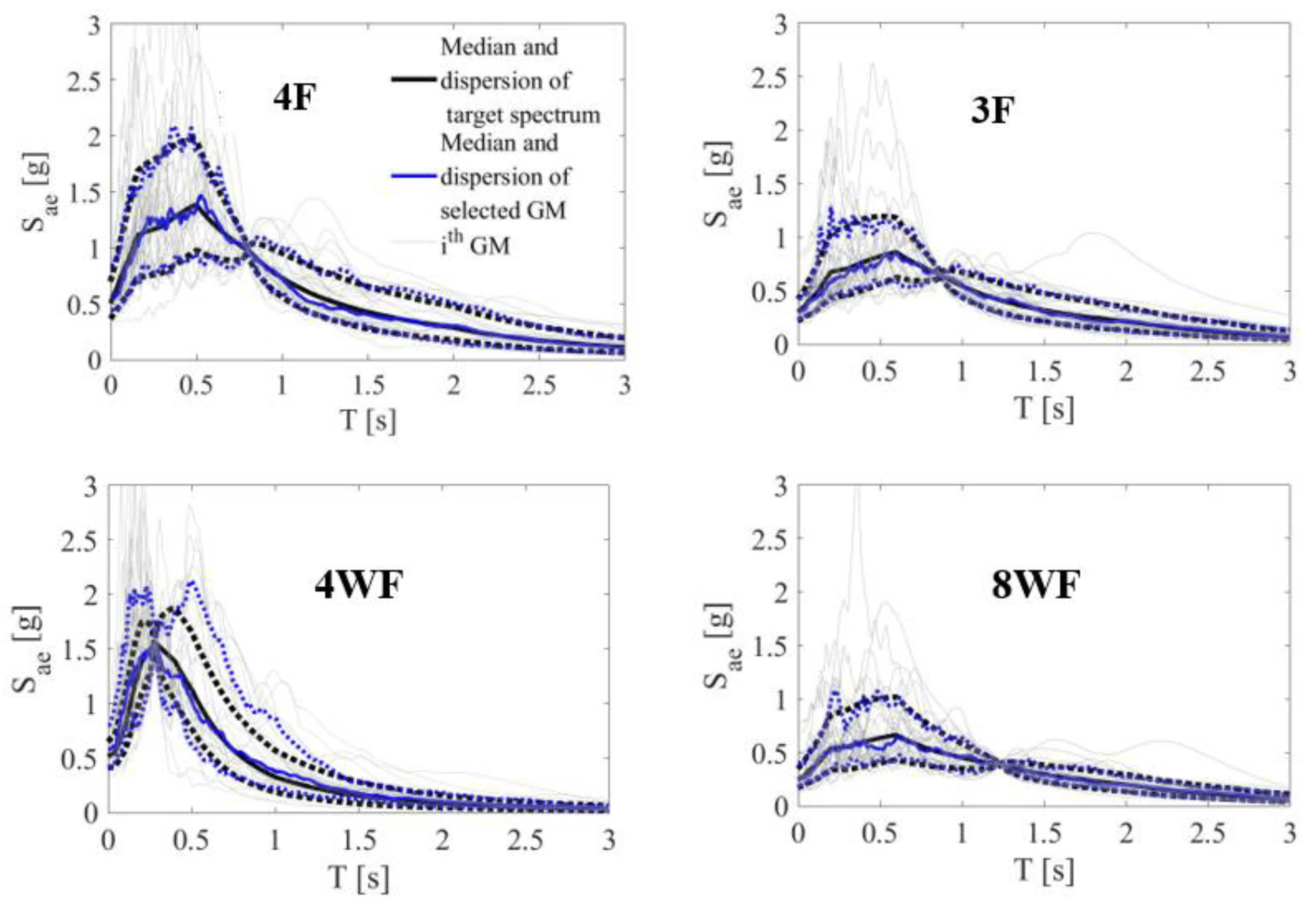
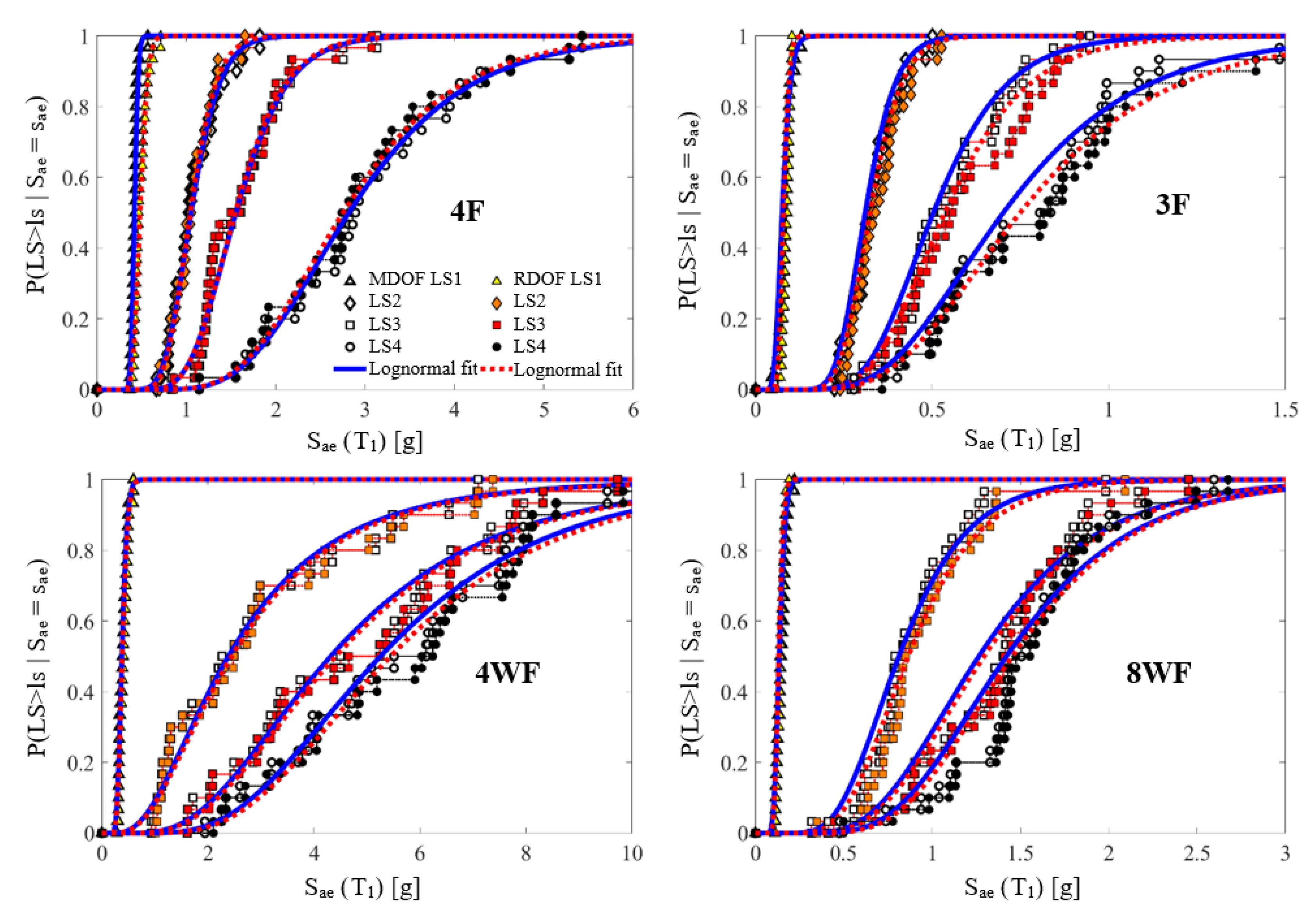
4.2. Incremental Dynamic Analysis (IDA) and Fragility Analysis

The capabilities of RDOF models were evaluated by performing an incremental dynamic analysis (IDA) [39] and seismic fragility analysis considering a set of thirty hazard-consistent ground motions (GMs). The ground motions were selected by the ground motion selection algorithm [40], where the target spectra were defined by conditional spectra (CS) [41]. The CS was determined based on the official seismotectonic model of the region of Slovenia [42], considering the location of Ljubljana, Slovenia, and spectral acceleration corresponding to the return period of 2475 years at the fundamental period of each building model. Further on, the variation of the soil type was taken into account. Both 4F building and 3F building were considered located on the soil type B [28], while 4WF and 8WF buildings were assumed to be located at soil type C. The ground motions (GMs) were selected from the NGA database [43] and RESORCE database [44]. Consequently, one set of GMs was selected for each investigated building. The median, 16th, and 84th percentile target spectra and the corresponding spectra of selected GMs, along with spectra of particular ground motion, are presented in Figure 8.

Differences between the IDA curves obtained by the two types of building models were observed in the format of spectral accelerations ${\mathrm{S}}_{\mathrm{ae}}$ at the fundamental period of buildings’ model versus maximum storey drift (Figure 9) and ${\mathrm{S}}_{\mathrm{ae}}$ at the fundamental period of the buildings’ model versus maximum storey acceleration (Figure 10). Storey drift IDA curves of the two building models are very similar in the case of the median IDA curve and when IDA curves are compared for each ground motion. The differences are observed for some ground motions only in a highly nonlinear range close to dynamic instability termed herein as the collapse. From Figure 10, it can be concluded that RDOF models can predict the storey acceleration and not only storey drifts. This is quite an important conclusion, because it is well known that the acceleration sensitive components can contribute significantly to the expected losses of building components [6,45,46].

Besides the IDA curve, limit-state points are also shown. The difference in limit-state drifts can be quite significant, especially for LS4. The difference is somewhat numerically based because the limit-state points were calculated only to a certain tolerance in terms of spectral acceleration at the fundamental period of building models. Thus, the difference in the limit-state drifts obtained by the RDOF and MDOF model increases with the intensity of the nonlinear effect. The most significant differences in indicated limit-state storey drifts can be observed for LS4 (Figure 9), where the IDA curves are almost flat. It should be noted that such differences in limit-state drifts are acceptable. Namely, a more precise estimation of the limit-state drifts is not required because the limit-state spectral accelerations are used for the seismic fragility analysis.

The limit-state spectral accelerations evaluated with IDA were used to estimate fragility functions in the form of a lognormal cumulative distribution function [1]. The estimated median limit-state spectral accelerations thus defined the fragility functions at the fundamental buildings’ periods, $\widetilde{{\mathrm{S}}_{\mathrm{ae},\mathrm{LS}} }$, and the corresponding standard deviation of logarithmic values of limit state spectral accelerations, ${\mathsf{\beta }}_{\mathrm{LS}}$. Based on the estimated parameters, the lognormal fragility functions were evaluated for all the considered limit states, both types of building models, and all investigated buildings (Figure 11). Fragility functions based on lognormal cumulative distribution function are also compared to empirical (sample-based) cumulative distribution functions, which were evaluated directly from the estimated sample of limit-state spectral accelerations. It can be observed that there are no significant differences in fragility functions obtained, considering the RDOF models (IFB or RDOF wall–frame) and conventional MDOF model for all the limit states of 4F, 3F, 4WF, and 8WF buildings (Figure 11). A good match of fragility functions is a logical result due to low differences between IDA curves based on RDOF and MDOF models presented in Figure 9 and Figure 10. For 3F building, some differences can be observed for the fragility functions for LS3 and LS4. The differences are mainly due to the torsional response of 3F building. Nevertheless, the significantly reduced degrees of freedom in the IFB model makes the RDOF models computationally very robust, which is necessary for a seismic fragility analysis.

The parameters of fragility functions, $\widetilde{{\mathrm{S}}_{\mathrm{ae},\mathrm{LS}} }$ and ${\mathsf{\beta }}_{\mathrm{LS}}$, are presented for all considered limit-states of the investigated buildings in

Table 2. The limit-state spectral accelerations at the fundamental buildings’ periods $\widetilde{{\mathrm{S}}_{\mathrm{ae},\mathrm{LS}}}$, the corresponding standard deviation of limit-state spectral accelerations in logarithmic values ${\mathsf{\beta }}_{\mathrm{LS}}$, and the corresponding error ${\mathsf{\epsilon }}_{\mathrm{R}/\mathrm{M}}$ for measuring the difference between the results based on the RDOF and MDOF models of 4F, 3F, 4WF, and 8WF buildings. If the limit-state $\widetilde{{\mathrm{S}}_{\mathrm{ae},\mathrm{LS}} }$ of the RDOF and MDOF model are equal, the nonzero error is the consequence of rounding decimals of the considered parameters.

−		$\widetilde{{\mathbf{S}}_{\mathbf{ae},\mathbf{LS}}} \left[\mathbf{g}\right]$			${\mathsf{\beta }}_{\mathbf{LS}}$
	Limit State	RDOF Model	MDOF Model	${\epsilon }_{R/M}$	RDOF Model	MDOF Model	${\epsilon }_{R/M}$
4F	LS1	0.47	0.42	+12%	0.14	0.10	+35%
	LS2	1.05	1.05	−1%	0.22	0.24	−8%
	LS3	1.55	1.56	−1%	0.28	0.29	−2%
	LS4	2.75	2.83	−2%	0.36	0.35	+7%
3F	LS1	0.08	0.08	+5%	0.15	0.23	−35%
	LS2	0.32	0.31	+4%	0.22	0.22	+1%
	LS3	0.54	0.50	+6%	0.34	0.32	+6%
	LS4	0.75	0.70	+7%	0.43	0.42	+2%
4WF	LS1	0.38	0.38	+2%	0.21	0.21	+2%
	LS2	2.45	2.38	+3%	0.65	0.65	−1%
	LS3	4.41	4.32	+2%	0.55	0.55	−1%
	LS4	5.45	5.26	+4%	0.48	0.48	−1%
8WF	LS1	0.13	0.13	+0%	0.16	0.19	−18%
	LS2	0.86	0.81	+6%	0.37	0.37	−1%
	LS3	1.15	1.07	+6%	0.42	0.42	−2%
	LS4	1.26	1.24	+2%	0.43	0.44	−2%

, where the relative error ${\mathsf{\epsilon }}_{\mathrm{R}/\mathrm{M}}$ was defined to evaluate the error of different parameters estimated with IFB or RDOF models to those calculated with the MDOF model. For median spectral accelerations, the error ${\mathsf{\epsilon }}_{\mathrm{R}/\mathrm{M}}$ for all the limit states of all investigated buildings does not exceed 12%, which can also be considered a promising result, especially because the largest error is observed in the case of LS1 for 4F building, which is not significant for loss or fatality risk estimation. The highest error is assessed for median $\widetilde{{\mathrm{S}}_{\mathrm{ae},\mathrm{LS}1}}$ and ${\mathsf{\beta }}_{\mathrm{LS}1}$ for the first limit state for 4F building and the parameter ${\mathsf{\beta }}_{\mathrm{LS}1}$for 3F building, which is, in both cases, due to slight differences in the estimated initial stiffness of the IFB models compared to the corresponding stiffness of the MDOF model. These differences are due to the simplified procedures of estimating the IFB model’s parameters and the high reduction in the degrees of freedom of the building model. It should be emphasized that a high level of relative errors is related to the low seismic intensity levels, where a slight absolute deviation can result in a high estimated relative error. For all the other limit states and investigated buildings (e.g., 4F, 3F, 4WF, and 8WF building), the error ${\mathsf{\epsilon }}_{\mathrm{R}/\mathrm{M}}$ for $\widetilde{{\mathrm{S}}_{\mathrm{ae},\mathrm{LS}} }$ estimated with the RDOF model does not exceed 7% (Table 2), which is a promising result.

Although the RDOF models have significantly fewer degrees of freedom, their capabilities are promising. The computational efficiency and robustness of the presented RDOF models are some of its most important advantages. The difference in computational time and the computational robustness for performing nonlinear dynamic analyses based on RDOF models and MDOF models largely depends on the ratio between the number of elements of building models [13]. Because the structural design of the analyzed buildings presented in this study is quite simple, the ratio between the sum of computational times is not so enormous but still significant. For example, for the RDOF models, the computational time for IDA was 9, 4, 14, and 18 h while for the MDOF model, it was 53, 17, 24, and 34 h for 4F, 3F, 4WF and 8WF buildings, respectively. Thus, the computational time is relatively lower for the presented simplified models than for the MDOF models. However, for the more complex design of building structures consisting of a significantly higher number of structural elements, the difference in computational times increases significantly [13]. Nevertheless, the numerical robustness is improved considerably. The RDOF models can be used for seismic analysis of building stock where it would not be possible to run all the cases manually. However, further developments are needed to make the RDOF model appropriate for many types of buildings and not only for predominantly symmetric reinforced concrete frame buildings with simple cantilever walls.

5. Conclusions

The reduced-degree-of-freedom (RDOF) model for seismic analysis of predominantly plan-symmetric reinforced concrete wall–frame building was introduced. The RDOF model was defined by combining the IFB model and the elastic beam-column elements with concentrated plasticity (i.e., plastic hinges), which are used to simulate the reinforced concrete frame and cantilever walls. The condensation of degrees-of-freedom of RDOF models was validated by the imposed cyclic displacement analysis for the frame and wall–frame buildings. For the investigated buildings, it was realized that the RDOF models of the frames (i.e., IFB models) and simple wall–frame buildings are quite accurate for predicting the storey shear – storey drift relationship. As a consequence, the RDOF models provided practically equal median IDA curves as the conventional MDOF models. Some differences in IDA curves for particular ground motions were observed for the range close to the dynamic instability of structures. However, the differences were not reflected in the near-collapse limit-state spectral accelerations at the fundamental buildings’ periods and the corresponding standard deviation of logarithmic values of the near-collapse limit-state spectral accelerations. Therefore, the RDOF models of the investigated buildings are sufficient for the prediction of fragility functions for different limit states.

The RDOF models of the investigated buildings are computationally robust and time-efficient. Thus, they can be used for response history analysis of building stock and for preliminary seismic risk analysis, which can serve as a basis for decision-making about the process of renovation of the building.

The RDOF models can be defined directly from the building stock information model. In this paper, the RDOF models were defined by utilizing the same building information model as for the MDOF models. However, algorithms for the generation of RDOF models based on incomplete building stock information models have to be developed for their practical applications in building stock loss estimation based on response history analysis. However, the demonstrated RDOF models can be used for seismic analysis of relatively simple frame or wall–frame buildings. Therefore, the RDOF models have to be further developed to be capable of simulating plan-irregular wall–frame buildings and other types of buildings.

References

1. Ibarra, L.F.; Krawinkler, H. Global Collapse of Frame Structures under Seismic Excitations. Ph.D. Thesis, Stanford University, Stanford, CA, USA, 2005. [Google Scholar]
2. Haselton, C.B.; Goulet, C.A.; Mitrani-Reiser, J.; Beck, J.L.; Deierlein, G.G.; Porter, K.A.; Stewart, J.P.; Taciroglu, E. An Assessment to Benchmark the Seismic Performance of a Code-Conforming Reinforced Concrete Moment-Frame Building; University of California at Berkeley: Berkeley, CA, USA, 2008. [Google Scholar]
3. Fajfar, P.; Dolšek, M.; Marušić, D.; Stratan, A. Pre- and post-test mathematical modelling of a plan-asymmetric reinforced concrete frame building. Earthq. Eng. Struct. Dyn. 2006, 35, 1359–1379. [Google Scholar] [CrossRef]
4. ATC. FEMA-P-58-1—Seismic Performance Assessment of Buildings, Volume 1—Methodology; FEMA: Washington, UK, 2018. [Google Scholar]
5. Fajfar, P. A non-linear analysis method for performance based seismic design. Earthq. Spec. 2000, 16, 573–592. [Google Scholar] [CrossRef]
6. Snoj, J.; Dolšek, M. Pushover-based seismic risk assessment and loss estimation of masonry buildings. Earthq. Eng. Struct. Dyn. 2020, 49, 567–588. [Google Scholar] [CrossRef]
7. Crowley, H.; Pinho, R.; van Elk, J.; Uilenreef, J. Probabilistic damage assessment of buildings due to induced seismicity. Bull. Earthq. Eng. 2019, 17, 4495–4516. [Google Scholar] [CrossRef]
8. Ogawa, K.; Kamura, H.; Inoue, K. Modeling of the moment resistant frame to fishbone-shaped frame for the response analy-sis. J. Str. Constr. Eng. 1999, 521, 119–126. [Google Scholar] [CrossRef]
9. Nakashima, M.; Ogawa, K.; Inoue, K. Generic frame model for simulation of earthquake responses of steel moment frames. Earthq. Eng. Struct. Dyn. 2002, 31, 671–692. [Google Scholar] [CrossRef]
10. Khaloo, A.R.; Khosravi, H. Modified fish-bone model: A simplified MDOF model for simulation of seismic responses of mo-ment resisting frames. Soil Dyn. Earth. Eng. 2013, 55, 195–210. [Google Scholar] [CrossRef]
11. Khaloo, A.R.; Khosravi, H.; Jamnani, H.H. Nonlinear Interstory Drift Contours for Idealised Forward Directivity Pulses us-ing “Modified Fish-Bone” Models. Adv. Str. Eng. 2015, 18, 603–627. [Google Scholar] [CrossRef]
12. Soleimani, R.; Khosravi, H.; Hamidi, H. Substitute Frame and adapted Fish-Bone model: Two simplified frames representa-tive of RC moment resisting frames. Eng. Struct. 2019, 185, 68–89. [Google Scholar] [CrossRef]
13. Jamšek, A.; Dolšek, M. Seismic analysis of older and contemporary reinforced concrete frames with the improved fish-bone model. Eng. Struct. 2020, 212, 110514. [Google Scholar] [CrossRef]
14. Luco, N.; Mori, Y.; Funahashi, Y.; Cornell, C.A.; Nakashima, M. Evaluation of predictors of non-linear seismic demands using ?fishbone? models of SMRF buildings. Earthq. Eng. Struct. Dyn. 2003, 32, 2267–2288. [Google Scholar] [CrossRef]
15. Haghighat, A.; Sharifi, A. Evaluation of Modified Fish-Bone Model for Estimating Seismic Demands of Irregular MRF Struc-tures. Period. Polytech. Civ. Eng. 2018. Available online: https://www.semanticscholar.org/paper/Evaluation-of-Modified-Fish-Bone-Model-for-Seismic-Haghighat-Sharifi/16e6980ed9e8163a2ac800238b2393606101840b (accessed on 10th December 2019). [CrossRef] [Green Version]
16. Li, X.; Kurata, M. Probabilistic updating of fish-bone model for assessing seismic damage to beam–column connections in steel moment-resisting frames. Comput. Aided Civ. Infrastruct. Eng. 2019, 34, 790–805. [Google Scholar] [CrossRef]
17. Zhe, Q.; Ting, G.; Qiqi, L.; Tao, W. Evaluation of the fishbone model in simulating the seismic response of multistory rein-forced concrete moment-resisting frames. Earthq. Eng. Eng. Vibr. 2019, 18, 315–330. [Google Scholar]
18. Araki, Y.; Ohno, M.; Mukai, I.; Hashimoto, N. Consistent DOF reduction of tall steel frames. Earthq. Eng. Struct. Dyn. 2017, 46, 1581–1597. [Google Scholar] [CrossRef]
19. FEMA 440. Improvement of Nonlinear Static Seismic Analysis Procedures; FEMA: Washington, UK, 2005. [Google Scholar]
20. Miranda, E.; Akkar, S.D. Generalised Interstory Drift Spectrum. J. Struct. Eng. 2006, 132, 840–852. [Google Scholar] [CrossRef] [Green Version]
21. Ramirez, C.M.; Miranda, E. Building-Specific Loss Estimation Methods & Tools for Simplified Performance-Based Earthquake Engineering. Ph.D. Thesis, Stanford University, Stanford, CA, USA, 2009. [Google Scholar]
22. Kilar, V.; Fajfar, P. Simplified Pushover Analysis of Building Structures. In Proceedings of the Eleventh World Conference on Earthquake Engineering, Acapulco, Mexico, 23–28 June 1996. [Google Scholar]
23. Kilar, V.; Fajfar, P. Simple Push-Over Analysis of Asymmetric Buildings. Earthq. Eng. Struct. Dyn. 1997, 26, 233–249. [Google Scholar] [CrossRef]
24. Dolšek, M. Development of computing environment for the seismic performance assessment of reinforced concrete frames by using simplified non-linear models. Bull. Earthq Eng. 2010, 8, 1309–1329. [Google Scholar] [CrossRef]
25. Fischinger, M.; Isaković, T.; Kolozvari, K.; Wallace, J. Guest editorial: Non-linear modelling of reinforced concrete structural walls. Bull. Earth. Eng. 2019, 17, 6359–6368. [Google Scholar] [CrossRef]
26. Celarec, D.; Dolšek, M. Practice-oriented probabilistic seismic performance assessment of infilled frames with consideration of shear failure of columns. Earthq. Eng. Struct. Dyn. 2012, 42, 1339–1360. [Google Scholar] [CrossRef]
27. CEN. Eurocode 2: Design of Concrete Structures—Part 1-1: General Rules and Rules for Buildings; European Committee for Standardization: Brussels, Belgium, 2004. [Google Scholar]
28. CEN. Eurocode 8: Design of Structures for Earthquake Resistance—Part 1: General Rules, Seismic Actions and Rules for Buildings; European Committee for Standardization: Brussels, Belgium, 2004. [Google Scholar]
29. Jamšek, A. Seismic stress test with incomplete building data (“Seizmični stresni test z nepopolnimi podatki o stavbi”), in Slo-vene. PhD Thesis, University of Ljubljana, Ljubljana, Slovenia, 2020. [Google Scholar]
30. Kosič, M. Determination of Dispersion Measures for Seismic Response of Concrete Buildings (“Določanje Raztrosa Potresnega odziva Armiranobetonskih Stavb”). Ph D. Thesis, University of Ljubljana, Ljubljana, Slovenia, 2014. [Google Scholar]
31. CEN. Eurocode 8: Design of Structures for Earthquake Resistance—Part 3: Assessment and Retrofitting of Buildings; European Committee for Standardization: Brussels, Belgium, 2005. [Google Scholar]
32. Negro, P.; Colombo, A. Irregularities induced by non-structural masonry panels in framed buildings. Eng. Struct. 1997, 19, 576–585. [Google Scholar] [CrossRef]
33. Fardis, M.N. (Ed.) Experimental and Numerical Investigations on the Seismic Response of RC Infilled Frames and Recommen-Dations for Code Provisions; LNEC: Lisbon, Portugal, 1996. [Google Scholar]
34. Fardis, M.N.; Negro, P. (Eds.) Seismic performance assessment and rehabilitation of existing buildings. In Proceedings of the International Workshop, EC JRC, Ispra, Italy, 4–5 April 2005. [Google Scholar]
35. CEN. Eurocode 8: Design of Structures for Earthquake Resistance—Part 2: Bridges; European Committee for Standardization: Brussels, Belgium, 2005. [Google Scholar]
36. MATLAB. The MathWorks, Inc. 2005. Available online: http://www.mathworks.com (accessed on 1 February 2012).
37. PEER. Open System for Earthquake Engineering Simulation (OpenSees); Pacific Earthquake Engineering Research Center: Berkeley, CA, USA, 2007. [Google Scholar]
38. FEMA 461. Interim Testing Protocols for Determining the Seismic Performance Characteristics of Structural and Nonstruc-tural Components; Federal Emergency Management Agency: Washington, UK, 2007. [Google Scholar]
39. Vamvatsikos, D.; Cornell, C.A. Incremental dynamic analysis. Earthq. Eng. Struct. Dyn. 2002, 31, 491–514. [Google Scholar] [CrossRef]
40. Jayaram, N.; Lin, A.T.; Baker, J. A Computationally Efficient Ground-Motion Selection Algorithm for Matching a Target Response Spectrum Mean and Variance. Earthq. Spectra 2011, 27, 797–815. [Google Scholar] [CrossRef]
41. Baker, J.W. Conditional Mean Spectrum: Tool for Ground-Motion Selection. J. Struct. Eng. 2011, 137, 322–331. [Google Scholar] [CrossRef]
42. Lapajne, J.; Motnikar, B.Š.; Zupančič, P. Probabilistic Seismic Hazard Assessment Methodology for Distributed Seismicity. Bull. Seism. Soc. Am. 2003, 93, 2502–2515. [Google Scholar] [CrossRef]
43. Chiou, B.S.J.; Darragh, R.; Gregor, N.; Silva, W.J. NGA Project Strong-Motion Database. Earthq. Spectra 2008, 24, 23–44. [Google Scholar] [CrossRef] [Green Version]
44. Akkar, S.; Sandikkaya, M.A.; Şenyurt, M.; Sisi, A.A.; Ay, B.Ő.; Traversa, P.; Douglas, J.; Cotton, F.; Luzi, L.; Hernandez, B.; et al. Reference database for seismic ground-motion in Europe (RESORCE). Bull. Earthq. Eng. 2014, 12, 311–339. [Google Scholar] [CrossRef] [Green Version]
45. Aslani, H.; Miranda, E. Probabilistic Earthquake Loss Estimation and Loss Disaggregation in Buildings. Ph D. Thesis, Stanford University, Stanford, CA, USA, 2005. [Google Scholar]
46. Bradley, B.A. Structure-Specific Probabilistic Seismic Risk Assessment. Ph D. Thesis, Engineering University of Canterbury Christchurch, New Zealand, 2009. Ph D. Thesis, Engineering University of Canterbury, Christchurch, New Zealand, 2009. [Google Scholar]
Figure 1. Schematic presentation of transition from (a) frame building to IFB model and (b) cantilever wall to elastic beam-column element with plastic hinges.
Buildings 11 00372 g001
Figure 2. Tri-linear moment-rotation relationship accounting for linear softening branch, characteristic points (p = 1, 2, 3) needed for the definition of moment-rotation relationship, and four limit states (LS1-LS4) for vertical structural elements (e.g., columns and walls).
Buildings 11 00372 g002
Figure 3. Schematic presentation of (a) the MDOF model and (b) the IFB model with the indication of characteristic moments of the plastic hinges and the corresponding indices.
Buildings 11 00372 g003
Figure 4. Schematic presentation of (a) MDOF model and (b) RDOF model of a simple wall–frame building.
Buildings 11 00372 g004
Figure 5. The elevation and plan views of the analyzed 4F, 3F, 4WF, and 8WF buildings.
Buildings 11 00372 g005
Figure 6. Storey shear – storey drift relationship based on imposed displacement analyses in first storey of IFB or RDOF models and MDOF models of 4F, 3F, 4WF, and 8WF buildings.
Buildings 11 00372 g006
Figure 7. Storey shear – storey drift relationship based on imposed displacement analyses, both types of building models (i.e., IFB and MDOF model) in the i-th storey for the imposed displacements in j-th storey of 4F building.
Buildings 11 00372 g007
Figure 8. The median, 16th, and 84th percentiles of target conditional spectra, the corresponding spectra of selected ground motions, and spectra of each ground motion selected for the incremental dynamic analysis (IDA) of 4F, 3F, 4WF, and 8WF buildings.
Buildings 11 00372 g008
Figure 9. IDA curves for each ground motion, the corresponding median IDA curve, and the limit-state points for the RDOF and MDOF model of 4F, 3F, 4WF, and 8WF building. IDA curves are presented in the format of spectral accelerations at the fundamental period of building, Sae(T1) versus maximum storey drift.
Buildings 11 00372 g009
Figure 10. IDA curves in the format of spectral accelerations at the fundamental period of a building, Sae(T1), versus maximum storey acceleration for the selected set of ground motions and the corresponding median for the RDOF and MDOF model of 4F, 3F, 4WF, and 8WF buildings.
Buildings 11 00372 g010
Figure 11. Fragility functions based on lognormal cumulative distribution functions and sample-based (empirical) fragility functions for all limit-states for RDOF and MDOF models of 4F, 3F, 4WF and 8WF buildings.
Buildings 11 00372 g011