
An Incentive-Based Optimization Approach for Load Scheduling Problem in Smart Building Communities


Abstract
:1. Introduction
1.1. Literature Review
1.2. Study Contributions
- The impact of thermal assets on the building energy consumption and human comfort are considered in the formulation.
- The user inconvenience levels for time-shiftable and thermal assets are considered in the formulation.
- The DR program participants’ incentives are included in the optimization model that helps them get incentivized based on the amount of energy they are willing to shift.
- For solving the nonlinear optimization problem, the method of feasible direction is discussed and employed.
- A complete data set for residential and office buildings’ appliances is prepared that can be used by other researchers in the field.
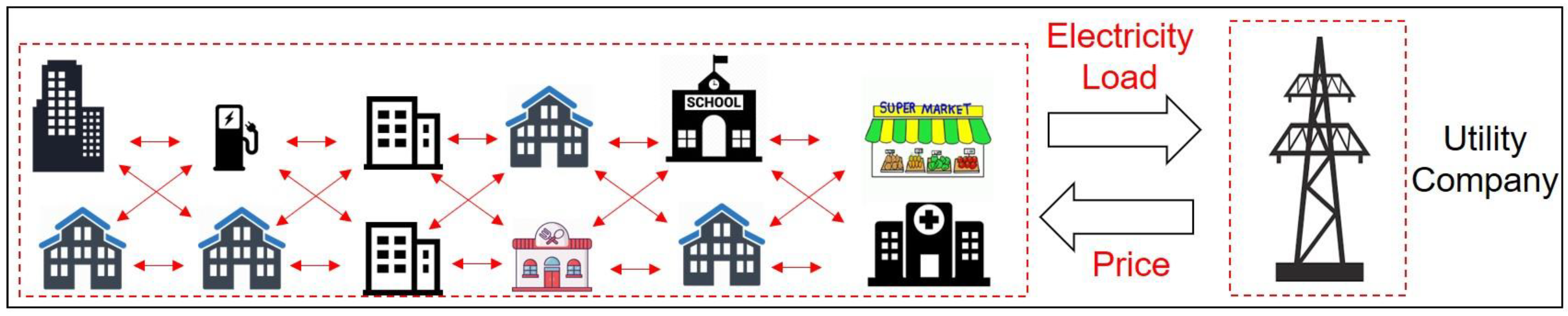
2. Problem Statement and Preliminaries
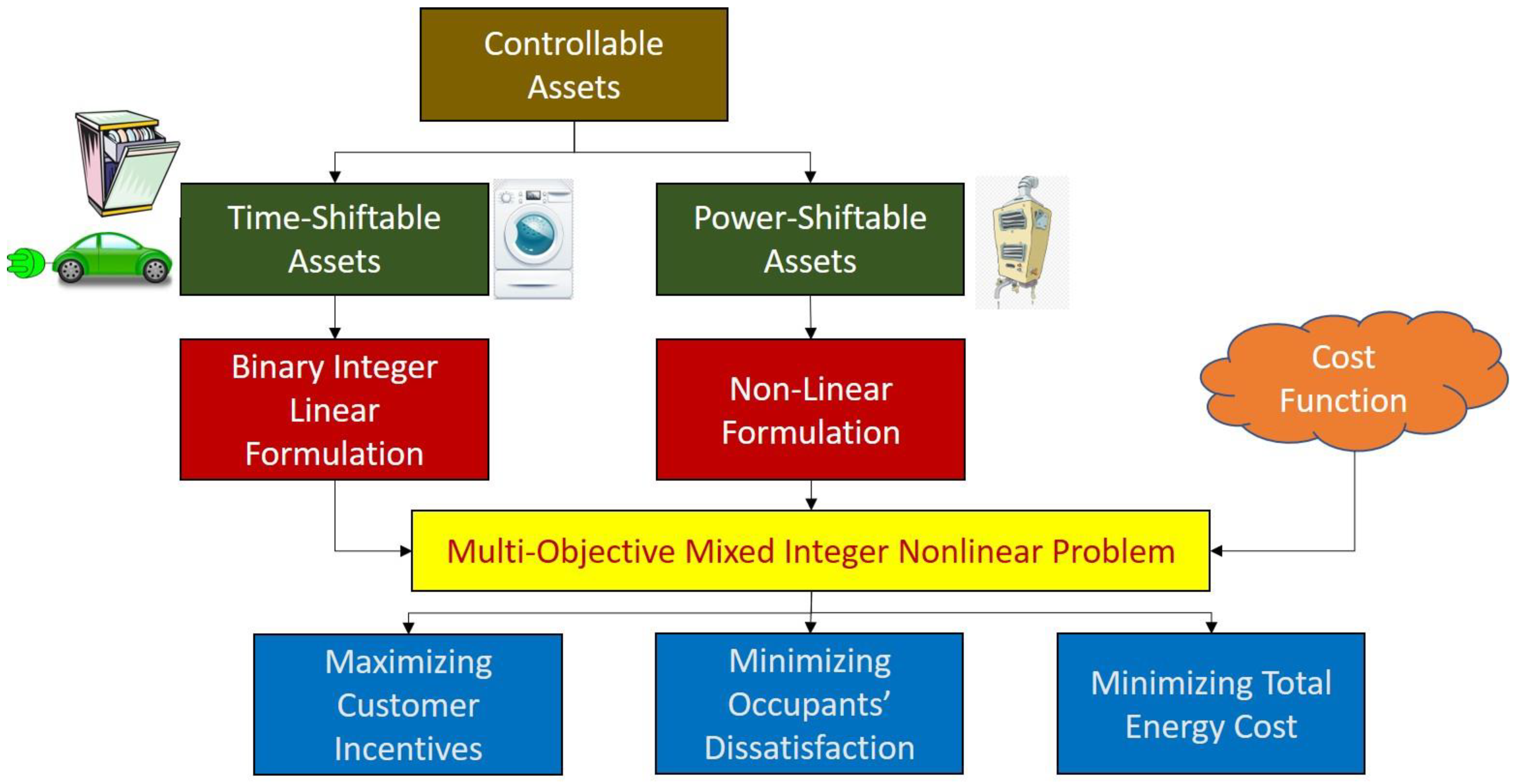
3. Problem Formulation
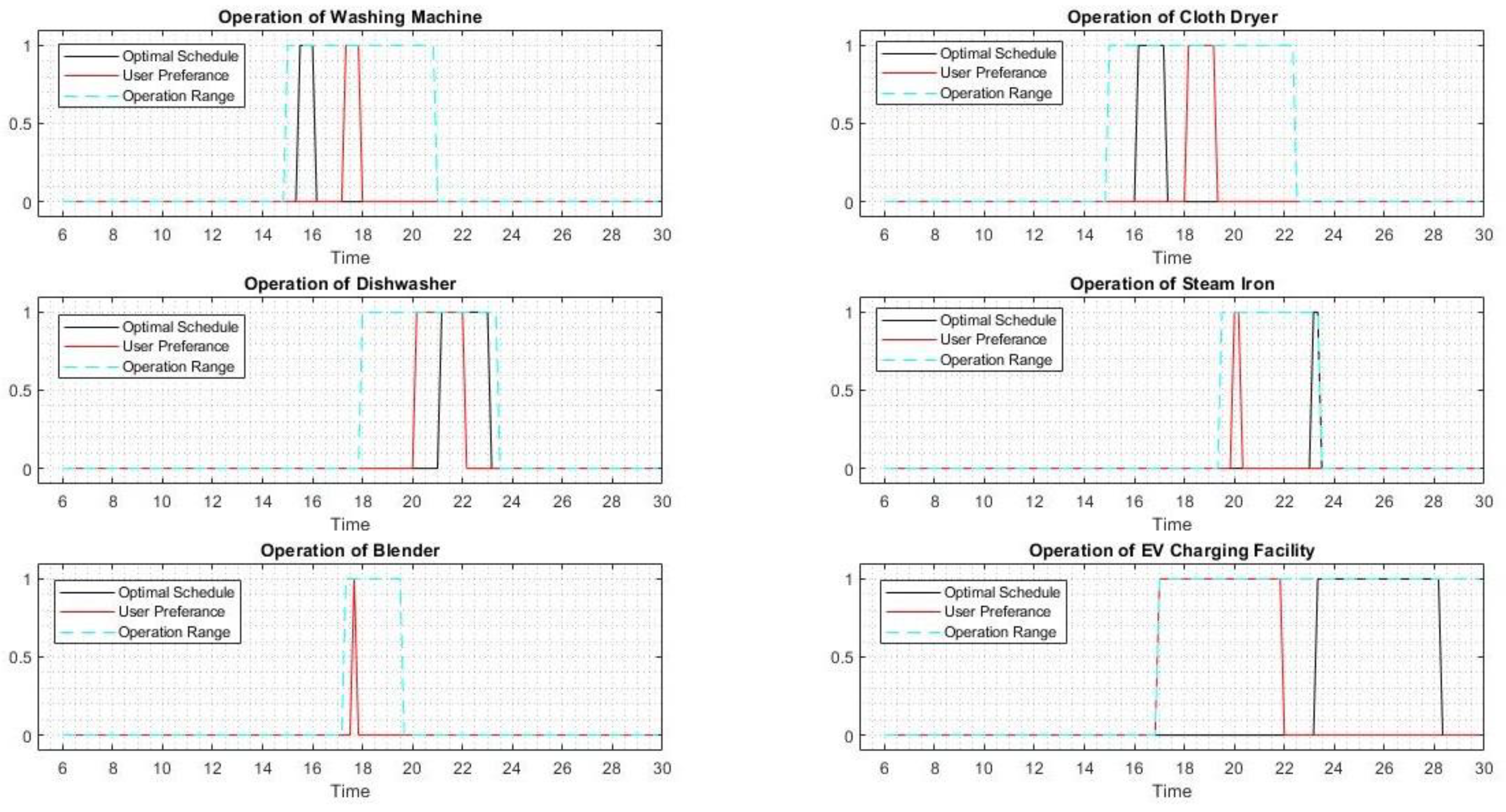
3.1. Time-Shiftable Assets
3.2. Thermal Assets
3.2.1. HVAC Systems
3.2.2. Electric Water Heater Systems
3.2.3. The Inconvenience Level for Thermal Assets
3.3. Objective Functions
3.4. The Optimization Model
3.5. The Solution Approach
4. Case Study Design
4.1. Case Scenarios
4.2. Building Functionalities
5. Results and Discussion
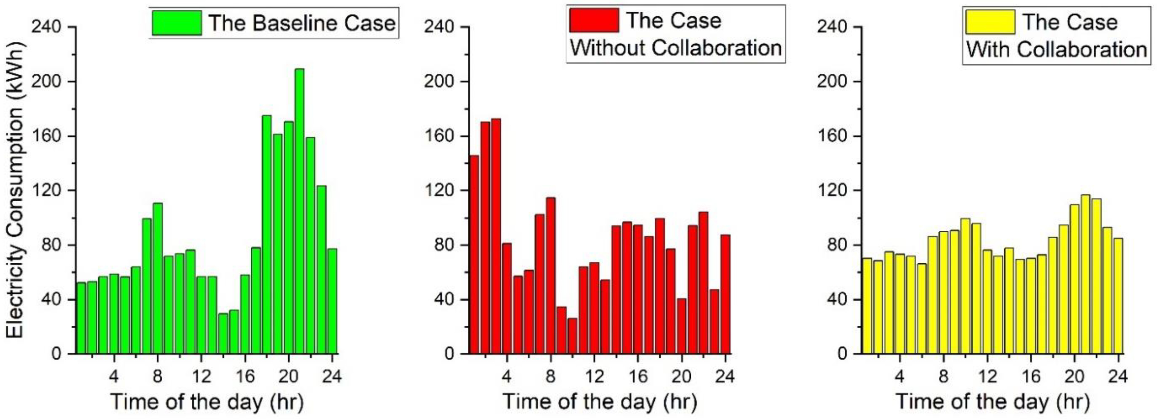
5.1. The Small-Scale Community
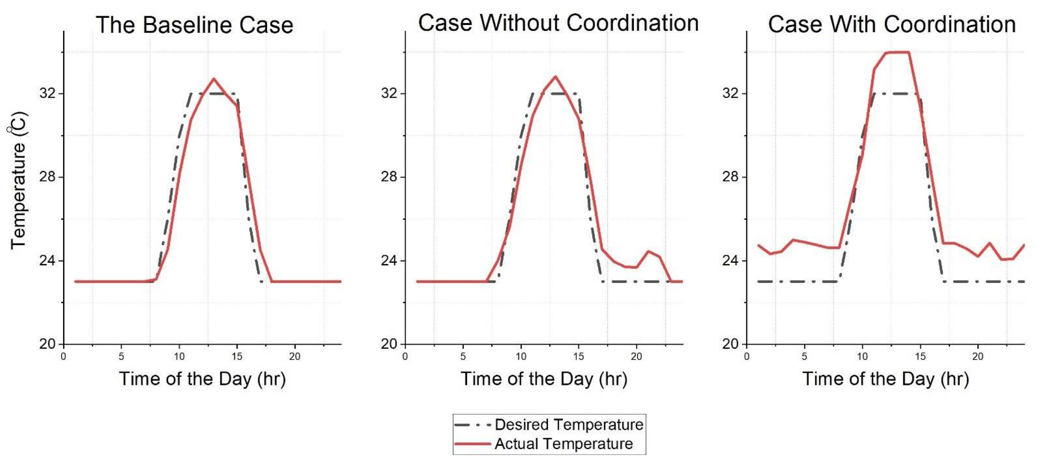
5.1.1. The Baseline Case
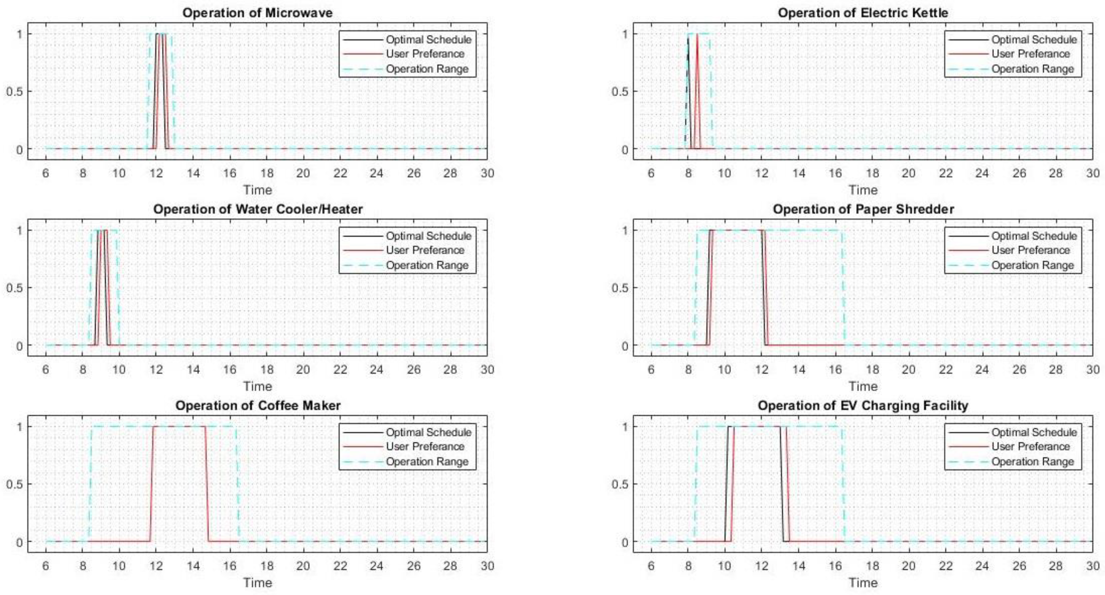
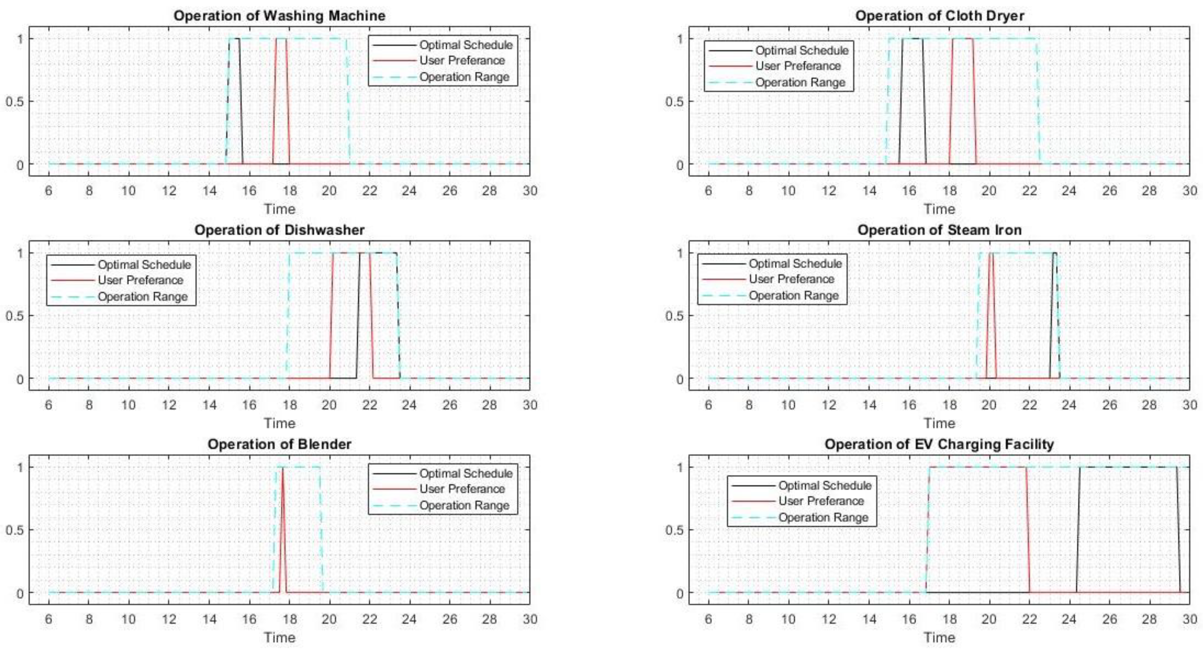
5.1.2. The Case without Building Collaboration
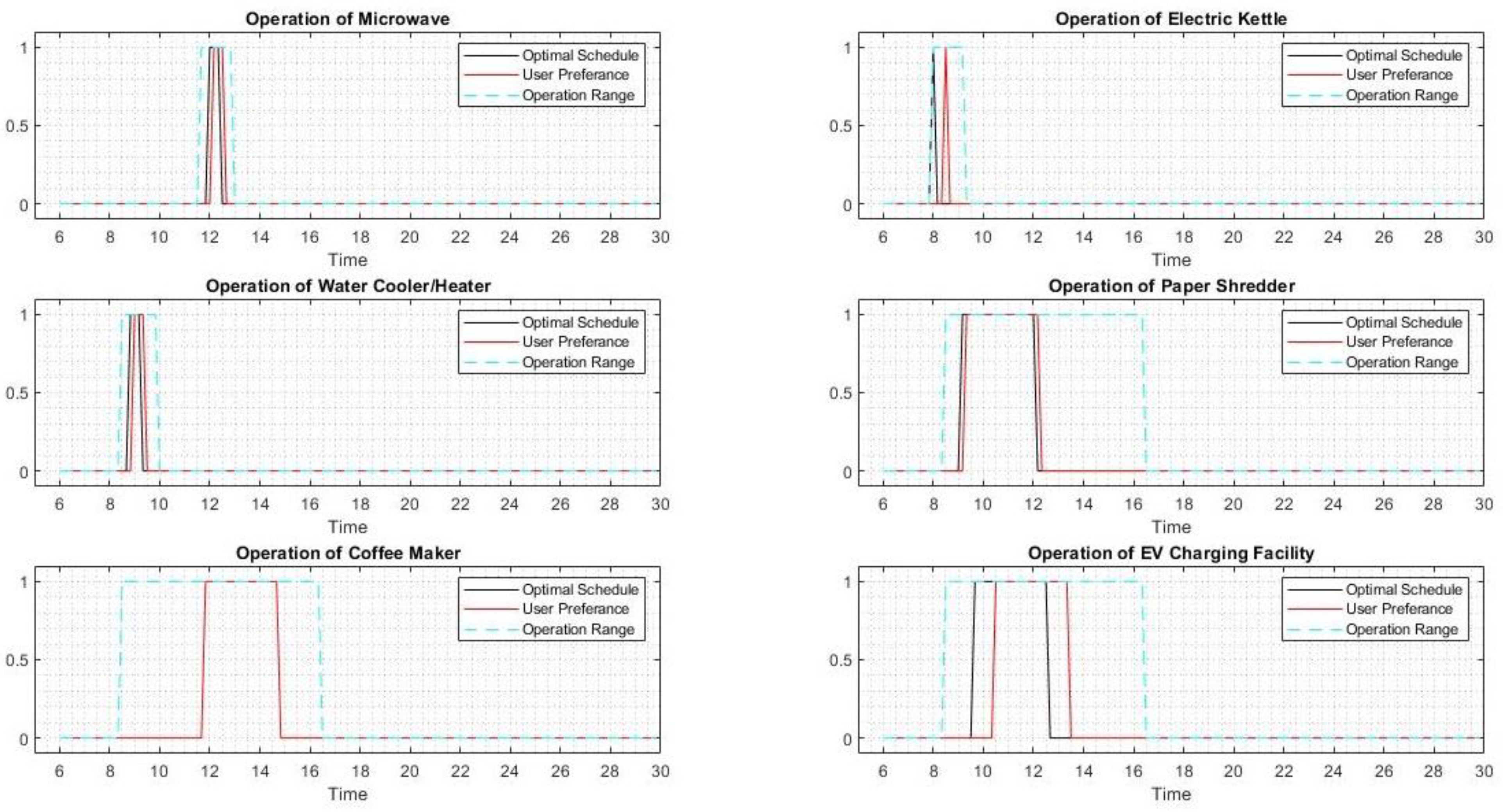
5.1.3. The Case with Building Collaboration
5.1.4. Comparison between Case Studies
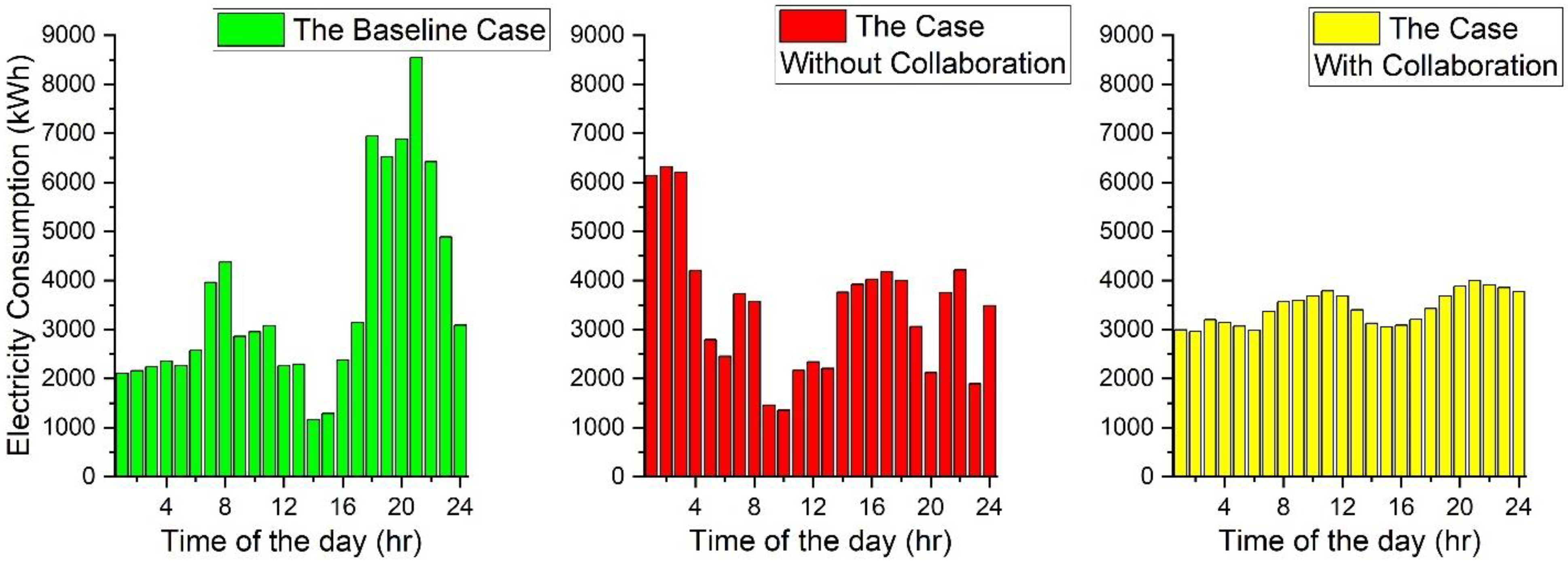
5.2. The Large-Scale Building Community
5.3. Discussion
6. Conclusions
Author Contributions
Funding
Institutional Review Board Statement
Informed Consent Statement
Data Availability Statement
Conflicts of Interest
Nomenclature
| a binary number to represent the optimal on or off status of a flexible time-shiftable asset i of building j at time t, which equals 1 if asset i is to be turned on at time t and zero otherwise | |
| an auxiliary binary decision variable to state the status operation of asset i of building j at time t. If , the operation of this asset is just completed during time slot t and the corresponding must be zero | |
| a binary number for the inconvenience, which equals 1 if there is a miss-match between the preferred schedule and the optimal schedule for deferrable asset i of building j at time t | |
| a binary number for incentives, which equals 1 if consumers earn incentives since they switched off asset i of building j at time t, against their preference, and zero otherwise | |
| the consumer’s preferred on-off status of a flexible time-shiftable asset i of building j at time t | |
| the inconvenience level for thermal asset i of building j at time t | |
| power consumption of the HVAC system in building j at time t (kW) | |
| power consumption of the EWH system in building j at time t (kW) | |
| building indoor temperature at time t () | |
| hot water temperature at time t () | |
| the start time of operation range for asset i of building j | |
| the end time of operation range for asset i of building j | |
| the required number of time slots to operate the time-shiftable asset i of building j | |
| the incentive offered at time t | |
| the time step length (h) | |
| rated power of time-shiftable asset i of building j | |
| start time | |
| planning horizon (h) | |
| factor of inertia | |
| difference between the actual temperature and the desired one () | |
| thermal conductivity (kW/) | |
| coefficient of performance | |
| mc | total thermal mass (kWh/) |
| the temperature of incoming water to the electric water heater system () | |
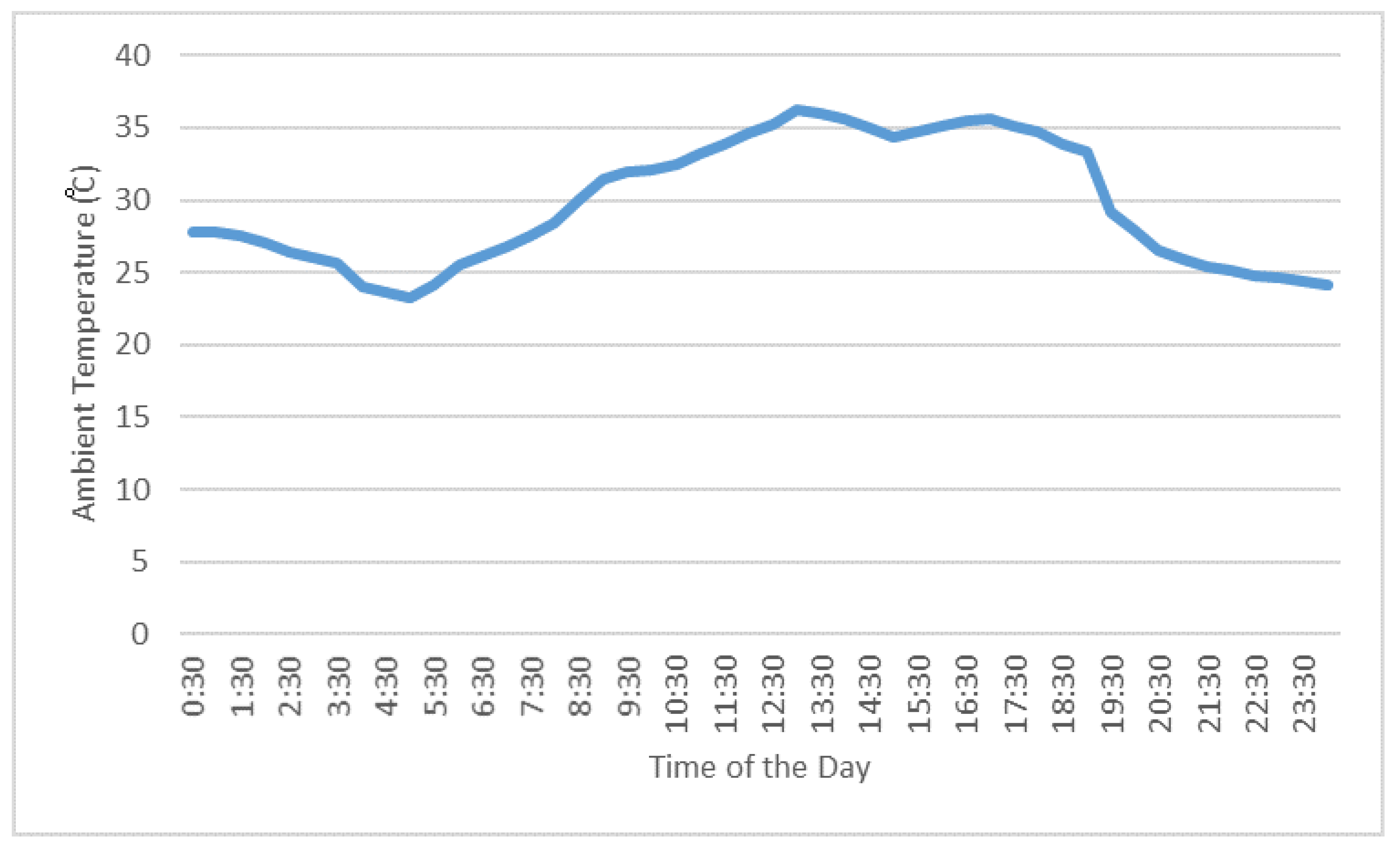
| ambient temperature () | |
| the capacity of the tank () | |
| the surface area of the tank () | |
| the density of water () | |
| the specific heat of water () | |
| the flow rate of water () | |
| total hourly load for building j | |
| R | the thermal resistance of the water storage tank () |
| maximum allowable difference between the desired temperature and actual temperature () | |
| , , | non-negative constants for the quadratic cost function |
| Indices | |
| i | index of building assets |
| j | index of buildings |
| t | index of time |
| Sets | |
| set of assets in building j | |
| set of buildings in the community | |
References
- Gelazanskas, L.; Gamage, K.A.A. Demand side management in smart grid: A review and proposals for future direction. Sustain. Cities Soc. 2014, 11, 22–30. [Google Scholar] [CrossRef]
- Yu, D.; Xu, X.; Dong, M.; Nojavan, S.; Jermsittiparsert, K. Modeling and prioritizing dynamic demand response programs in the electricity markets. Sustain. Cities Soc. 2020, 53, 101921. [Google Scholar] [CrossRef]
- Farzan, F.; Jafari, M.A.; Gong, J.; Farzan, F.; Stryker, A. A multi-scale adaptive model of residential energy demand. Appl. Energy 2015, 150, 258–273. [Google Scholar] [CrossRef]
- Missaoui, R.; Joumaa, H.; Ploix, S.; Bacha, S. Managing energy Smart Homes according to energy prices: Analysis of a Building Energy Management System. Energy Build. 2014, 71, 155–167. [Google Scholar] [CrossRef]
- Ghofrani, A.; Nazemi, S.D.; Jafari, M.A. Prediction of building indoor temperature response in variable air volume systems. J. Build. Perform. Simul. 2020, 13. [Google Scholar] [CrossRef]
- Ghofrani, A.; Nazemi, S.D.; Jafari, M.A. HVAC load synchronization in smart building communities. Sustain. Cities Soc. 2019, 51, 101741. [Google Scholar] [CrossRef]
- Zhou, B.; Li, W.; Wing, K.; Cao, Y.; Kuang, Y.; Liu, X.; Wang, X. Smart home energy management systems: Concept, con fi gurations, and scheduling strategies. Renew. Sustain. Energy Rev. 2016, 61, 30–40. [Google Scholar] [CrossRef]
- Benetti, G.; Caprino, D.; Della, M.L.; Facchinetti, T. Electric load management approaches for peak load reduction: A systematic literature review and state of the art. Sustain. Cities Soc. 2015, 20, 124–141. [Google Scholar] [CrossRef]
- Dong, B.; Lam, K.P. Journal of Building Performance Simulation Building energy and comfort management through occupant behaviour pattern detection based on a large-scale environmental sensor network. J. Build. Perform. Simul. 2011, 4, 359–369. [Google Scholar] [CrossRef]
- Chavali, P.; Yang, P.; Nehorai, A. A Distributed Algorithm of Appliance Scheduling for Home Energy Management System. IEEE Trans. Smart Grid 2014, 5, 282–290. [Google Scholar] [CrossRef]
- Chen, X.; Wei, T.; Hu, S. Uncertainty-Aware Household Appliance Scheduling Considering Dynamic Electricity Pricing in Smart Home. IEEE Trans. Smart Grid 2013, 4, 932–941. [Google Scholar] [CrossRef]
- Chen, C.; Wang, J.; Heo, Y.; Kishore, S. MPC-Based Appliance Scheduling for Residential Building Energy Management Controller. IEEE Trans. Smart Grid 2013, 4, 1401–1410. [Google Scholar] [CrossRef]
- Sou, K.C.; Weimer, J.; Sandberg, H.; Johansson, K.H. Scheduling Smart Home Appliances Using Mixed Integer Linear Programming. In Proceedings of the 2011 50th IEEE Conference on Decision and Control and European Control Conference, Orlando, FL, USA, 12–15 December 2011; pp. 5144–5149. [Google Scholar] [CrossRef] [Green Version]
- Setlhaolo, D.; Xia, X. Optimal scheduling of household appliances incorporating appliance coordination. Energy Procedia 2014, 61, 198–202. [Google Scholar] [CrossRef] [Green Version]
- Izmitligil, H.; Ozkan, H.A. A Home Power Management System Using Mixed Integer Linear Programming for Scheduling Appliances and Power Resources. In Proceedings of the 2016 IEEE PES Innovative Smart Grid Technologies Conference Europe (ISGT-Europe), Ljubljana, Slovenia, 9–12 October 2016. [Google Scholar] [CrossRef]
- Ozkan, H.A. Appliance based control for Home Power Management Systems. Energy 2016, 114, 693–707. [Google Scholar] [CrossRef]
- Nazemi, S.D.; Jafari, M.A. An automated cluster-based approach for asset rescheduling in building communities. In Proceedings of the 2020 IEEE Texas Power and Energy Conference (TPEC), College Station, TX, USA, 6–7 February 2020. [Google Scholar] [CrossRef]
- Setlhaolo, D.; Xia, X.; Zhang, J. Optimal scheduling of household appliances for demand response. Electr. Power Syst. Res. 2014, 116, 24–28. [Google Scholar] [CrossRef]
- Setlhaolo, D.; Xia, X. Electrical Power and Energy Systems Combined residential demand side management strategies with coordination and economic analysis. Int. J. Electr. Power Energy Syst. 2016, 79, 150–160. [Google Scholar] [CrossRef]
- Nazemi, S.D.; Zaidan, E.; Jafari, M.A. The Impact of Occupancy-Driven Models on Cooling Systems in Commercial Buildings. Energies 2021, 14, 1722. [Google Scholar] [CrossRef]
- Yahia, Z.; Pradhan, A. Optimal load scheduling of household appliances considering consumer preferences: An experimental analysis. Energy 2018, 163, 15–26. [Google Scholar] [CrossRef]
- Muhsen, D.H.; Haider, H.T.; Al-nidawi, Y.; Khatib, T. Optimal Home Energy Demand Management Based Multi-Criteria Decision Making Methods. Electronics 2019, 8, 524. [Google Scholar] [CrossRef] [Green Version]
- Yahia, Z.; Pradhan, A. Multi-objective optimization of household appliance scheduling problem considering consumer preference and peak load reduction. Sustain. Cities Soc. 2020, 55, 102058. [Google Scholar] [CrossRef]
- Rodrigues, J.J.P.C.; Solic, P.; Igor, R.S.; Rab, R.D.A.L.; Carvalho, A. A preference-based demand response mechanism for energy management in a microgrid. J. Clean. Prod. 2020, 255, 120034. [Google Scholar] [CrossRef]
- Caprino, D.; della Vedova, M.L.; Facchinetti, T. Peak shaving through real-time scheduling of household appliances. Energy Build. 2014, 75, 133–148. [Google Scholar] [CrossRef]
- Setlhaolo, D.; Xia, X. Optimal scheduling of household appliances with a battery storage system and coordination. Energy Build. 2015, 94, 61–70. [Google Scholar] [CrossRef]
- Shirazi, E.; Jadid, S. Optimal residential appliance scheduling under dynamic pricing scheme via HEMDAS. Energy Build. 2015, 93, 40–49. [Google Scholar] [CrossRef]
- Zhu, J.; Lin, Y.; Lei, W.; Liu, Y.; Tao, M. Optimal household appliances scheduling of multiple smart homes using an improved cooperative algorithm. Energy 2019, 171, 944–955. [Google Scholar] [CrossRef]
- Kinhekar, N.; Prasad, N.; Om, H. Multiobjective demand side management solutions for utilities with peak demand deficit. Int. J. Electr. Power Energy Syst. 2014, 55, 612–619. [Google Scholar] [CrossRef]
- Yalcintas, M.; Hagen, W.T.; Kaya, A. An analysis of load reduction and load shifting techniques in commercial and industrial buildings under dynamic electricity pricing schedules. Energy Build. 2015, 88, 15–24. [Google Scholar] [CrossRef]
- Vaziri, S.M.; Rezaee, B.; Monirian, M.A. Utilizing renewable energy sources ef fi ciently in hospitals using demand dispatch. Renew. Energy 2019. [Google Scholar] [CrossRef]
- Paudyal, P.; Ni, Z. Smart home energy optimization with incentives compensation from inconvenience for shifting electric appliances. Electr. Power Energy Syst. 2019, 109, 652–660. [Google Scholar] [CrossRef]
- Mohsenian-Rad, A.-H.; Wong, V.; Jatskevich, J.; Schober, R.; Leon-Garcia, A. Autonomous Demand-Side Management Based on Game-Theoretic Energy Consumption Scheduling for the Future Smart Grid. IEEE Trans. Smart Grid 2010, 1, 320–331. [Google Scholar] [CrossRef] [Green Version]
- Ipakchi, A.; Albuyeh, F. Grid of the Future. IEEE Power Energy Mag. 2009, 7, 52–62. [Google Scholar] [CrossRef]
- Hong, Y.; Lin, J.; Wu, C.; Chuang, C. Multi-Objective Air-Conditioning Control Considering Fuzzy Parameters Using Immune Clonal Selection Programming. IEEE Trans. Smart Grid 2012, 3, 1603–1610. [Google Scholar] [CrossRef]
- Black, J.W. Integrating Demand into the U.S. Electric Power System: Technical, Economic, and Regulatory Frameworks for Responsive Load. Ph.D. Thesis, Massachusetts Institute of Technology, Cambridge, MA, USA, 2005. [Google Scholar]
- Tiptipakorn, S.; Lee, W.-J. A Residential Consumer-Centered Load Control Strategy in Real-Time Electricity Pricing Environment. In Proceedings of the 2007 39th North American Power Symposium, Las Cruces, NM, USA, 30 September–2 October 2007. [Google Scholar]
- Rourke, P.; Schweppe, F.C. Space conditioning load under spot or time of day pricing. IEEE Trans. Power Appar. Syst. 1983, 5, 1294–1301. [Google Scholar] [CrossRef]
- Nehrir, M.H.; Jia, R.; Pierre, D.A.; Hammerstrom, D.J. Power Management of Aggregate Electric Water Heater Loads by Voltage Control. In Proceedings of the 2007 IEEE Power Engineering Society General Meeting, Tampa, FL, USA, 24–28 June 2007. [Google Scholar]
- Bazaraa, M.S.; Sherali, H.D.; Shetty, C.M. Nonlinear Programming: Theory and Algorithms, 3rd ed.; Wiley-Interscience: Hoboken, NJ, USA, 2006. [Google Scholar]


| No. | Asset | Rated Power (kW) | User Preferred Time | The Operation Range | Duration (Minutes) |
|---|---|---|---|---|---|
| 1 | Clothes washing machine | 3.5 | 17:20–18:00 | 15–21 | 40 |
| 2 | Clothes dryer | 3.2 | 18:10–19:20 | 15–22:30 | 70 |
| 3 | Dishwasher | 2.8 | 20:10–22:10 | 18–23:30 | 120 |
| 4 | Microwave | 0.9 | 18:30–18:40 | 18:20–19:10 | 10 |
| 5 | Electric kettle | 1.8 | 7:30–7:40 19–19:10 | 7:10–7:50 18:50–19:30 | 10 |
| 6 | Electric stove | 5.2 | 7–7:40 18–18:40 | 6:30–7:50 17:30–19:20 | 40 |
| 7 | Blender | 0.8 | 17:40–17:50 | 17:20–18:40 | 10 |
| 8 | Hair dryer | 1.5 | 6:40–6:50 | 6:30–8 | 10 |
| 9 | Steam iron | 1.4 | 20–20:20 | 19:30–23:30 | 20 |
| 10 | Vacuum cleaner | 1.35 | 19:30–20 | 14–21 | 30 |
| 11 | Coffee maker | 1.1 | 7:10–7:20 | 6:40–8 | 10 |
| 12 | Phone charger | 0.01 | 21:30–23:30 | 18–1 (next day) | 120 |
| No. | Asset | Rated Power (kW) | User Preferred Time | The Operation Range | Duration (Minutes) |
|---|---|---|---|---|---|
| 1 | Microwave | 0.9 | 12:10–12:20 12:20–12:30 12:30–12:40 | 11:40–13:00 | 10 |
| 2 | Electric kettle | 1.8 | 8:30–8:40 14–14:10 | 8:00–9:20 13:30–14:30 | 10 |
| 3 | Bottleless water cooler and heater | 5.1 | 9–9:30 14–14:30 | 8:30–10 12:30–15 | 30 |
| 4 | Paper shredder | 0.15 | 15–15:20 | 14–17 | 20 |
| 5 | Coffee maker | 1.1 | 8:20–8:30 11–11:10 14–14:10 | 8–8:40 10:30–11:30 13:30–15 | 10 |
| Building Type | Number of PEVs | User Preferred Time | The Operation Range | Charging Duration for One Car (mins) |
|---|---|---|---|---|
| Residential unit, Type 1 | 1 | 17–22 | 17–6 (next day) | 300 |
| Residential unit, Type 2 | 2 | 19–24 | 18:30–6 (next day) | 300 |
| Residential unit, Type 3 | 1 | 17–18 21–2 (next day) | 17–18 21–6 (next day) | 360 |
| Office building | 10 | 9–12 | 8:30–16:30 | 180 |
| Parameters | Value |
|---|---|
| Thermal conductivity | |
| The total thermal mass of the fluid of the cooling system | |
| The coefficient of performance of the cooling system | |
| The temperature of incoming water to the EWH system | |
| The volume of the storage tank of the EWH system | |
| The surface area of the storage tank of the EWH system | (m2) |
| The density of water | |
| The specific heat of water | |
| The thermal resistance of the water storage tank | R = 1.309(m2°C/W) |
| The flow rate of the hot water | |
| Power range of the EWH system | |
| Power range of the cooling system |
| Case | Energy Consumption Reduction | Peak Demand Reduction | Energy-Cost Saving | |
|---|---|---|---|---|
| Small-scale building community | Without collaboration | 3.98% | 17.35% | 8.76% |
| With collaboration | 5.31% | 44.15% | 10.47% | |
| Large-scale building community | Without collaboration | 4.05% | 26.13% | 9.91% |
| With collaboration | 5.43% | 53.15% | 13.02% | |
Publisher’s Note: MDPI stays neutral with regard to jurisdictional claims in published maps and institutional affiliations. |
© 2021 by the authors. Licensee MDPI, Basel, Switzerland. This article is an open access article distributed under the terms and conditions of the Creative Commons Attribution (CC BY) license (https://creativecommons.org/licenses/by/4.0/).
Share and Cite
Nazemi, S.D.; Jafari, M.A.; Zaidan, E. An Incentive-Based Optimization Approach for Load Scheduling Problem in Smart Building Communities. Buildings 2021, 11, 237. https://doi.org/10.3390/buildings11060237
Nazemi SD, Jafari MA, Zaidan E. An Incentive-Based Optimization Approach for Load Scheduling Problem in Smart Building Communities. Buildings. 2021; 11(6):237. https://doi.org/10.3390/buildings11060237
Chicago/Turabian StyleNazemi, Seyyed Danial, Mohsen A. Jafari, and Esmat Zaidan. 2021. "An Incentive-Based Optimization Approach for Load Scheduling Problem in Smart Building Communities" Buildings 11, no. 6: 237. https://doi.org/10.3390/buildings11060237