Agent Based Modelling of a Local Energy Market: A Study of the Economic Interactions between Autonomous PV Owners within a Micro-Grid

Abstract

Urban Photovoltaic (PV) systems can provide large fractions of the residential electric demand at socket parity (i.e., a cost below the household consumer price). This is obtained without necessarily installing electric storage or exploiting tax funded incentives. The benefits of aggregating the electric demand and renewable output of multiple households are known and established; in fact, regulations and pilot energy communities are being implemented worldwide. Financing and managing a shared urban PV system remains an unsolved issue, even when the profitability of the system as a whole is demonstrable. For this reason, an agent-based modelling environment has been developed and is presented in this study. It is assumed that an optimal system (optimized for self-sufficiency) is shared between 48 households in a local grid of a positive energy district. Different scenarios are explored and discussed, each varying in number of owners (agents who own a PV system) and their pricing behaviour. It has been found that a smaller number of investors (i.e., someone refuse to join) provokes an increase of the earnings for the remaining investors (from 8 to 74% of the baseline). Furthermore, the pricing strategy of an agent shows improvement potential without knowledge of the demand of others, and thus it has no privacy violations.

1. Introduction

1.1. The Problem of Climate Change Has Been Internationally Recognized, The Political Will Is in Place

Climate change is one of the main challenges that threaten the wellbeing or the very existence of human society. This threat cannot be ignored because it can impact a wide range of natural ecosystems and socio-technical systems (e.g., [1,2,3,4,5,6,7]). In the last few decades, numerous technologies have been discovered, or improved, that can dramatically reduce our greenhouse gas emissions: renewable or low carbon energy generation facilities, energy storage systems, energy efficiency, and carbon capture devices. The vast majority of countries and international institutions on the planet agree on the danger of climate change and on the need for action [8]. In other words, since the political and social will to build a low carbon economy has been largely achieved, the focus of this study has been put chiefly on practical strategies and effective transition pathways. The subject is how to achieve a transition to a low carbon society in an economically beneficial way and without causing discontent. To reach this goal, it is essential to analyze the impact of different market designs and the choices of different households in creating potentially harmful or unfair economic impacts.

1.2. How Change Can Happen

To transform the will for change to actual change, it is important to understand the causes and the mechanisms that activate the changes. According to Giddens’ study [9], an important role in the evolution of technology is played by the interaction between socio-technical regimes: (i) the existing dominating technology and the social structure it generated, and technological niches, (ii) newer, smaller and dynamic sociotechnical entities that disturb the existing regime. Geels and Schot [10] elaborated different transition pathways (which include transformation, reconfiguration, technological substitution, and de-alignment and re-alignment) elaborating upon previous work and criticisms. In particular, Geels [11] added new elements on the subject introducing the so called ‘socio-technical landscape’. The socio-technical landscape is the sum of morals, beliefs, knowledge, and ideas that can spur change in a socio-technical regime. Suarez and Oliva [12] presented different modifications of the socio-technical landscape: regular, hyper-turbulence, specific shock, disruptive, and avalanche. Also Scott [13] speaks about the forces that drive a transition or the conservation of a socio-technical regime, which can therefore be seen as a socio-technical landscape. These forces are divided into three groups: regulative (such as laws and standards), normative (such as values and norms), and cognitive (such as beliefs and search heuristics). The study argues that the stronger of these forces is the cognitive one since it is the most immersive and invisible for the actors under its influence. Other aspects that are fundamental in a transition are the selection pressure and the coordination of resources; these two are deeply interconnected according to Smith et al.’s findings [14]. Specific examples of cognitive forces are the attitudes of end users toward innovative technologies; a large amount of literature exists on this topic (see [15]), but the authors consider obtaining a low carbon economy [16] a rather difficult endeavor.

1.3. Existing Optimization of Urban PV Systems and Research Gap

The coordination of resources, in a practical sense, is of the utmost importance in the case of PV technology. PV technology is currently one of the best candidates to shift the main energy source of our civilization away from fossil fuels. The direct use of the energy from the sun offers an abundant renewable supply with no pollutant emissions during the operational phase, thus producing fewer environmental side effects per unit of energy used compared to the present global energy mix. In general, PV systems can be categorized as urban PV or free-standing utility scale. Urban PV, as the adjective claims, is located in cities on buildings or infrastructure and serves the energy need of its immediate surrounding; this category is the subject of this study. On the other end, free-standing utility scales operate similarly to a traditional power plant: the electricity is generated in a rather large facility, then transmitted and distributed by the wider electric grid.

Both these categories of photovoltaic systems have strengths and weaknesses compared to the other, but both are characterized by a prominence of the initial investment compared to the operational costs. In other words, it takes a long time to repay the initial investment, but after that, savings and revenues can be enjoyed at almost no cost. These characters cause the payback time to be long (over 10 years), even amidst positive Net Present Value (NPV) calculated with discount rate of about 3% (see [17]).

Numerous studies have tackled the economic feasibility of the urban PV systems in the past few years, highlighting different aspects in the results [18]. In particular, a number of studies have optimized the capacity and positions of PV systems according to their lifetime economic performance in self-consumption within the parent building or district (as briefly explained in Section 2.4) [19].

Lovati et al. [17] performed optimization over a school building where PV can be installed both on the roof and on a tilted façade. Most of the electric demand is in winter due to electric heating. Furthermore, summer break reduces demand during summer. The NPV maximization suggests a capacity of PV that can achieve a self-sufficiency above 30%. Moreover, part of the system is installed over the façade because of better self-consumption despite vast residual space on the roof.

Adami et al. [20] considered the differences in price between roof and façade solutions because of the premium paid for aesthetics and multi-functionality and the price reduction due to substitution of a cladding material. It shows that the optimal capacity on the façade is inversely proportional to its unitary price, and it starts to become advantageous when its unitary price falls below 2000 (€/kWp) (considering a unitary price on the roof of 1440 (€/kWp)).

Similarly, Vigna et al. [21] performed optimization over different building clusters (or districts) with varying urban density and functions. The residential function is shown in single family houses or larger high-rise buildings, and the larger buildings are also hypothesized with office or mixed electric demands. The procedure is repeated with two different reward functions: maximize Net Present Value (NPV) and maximize self-sufficiency. When the self-sufficiency is maximized, the office buildings are the best in performance thanks to the good matching between PV power production and building electricity demand (especially in summer). On the contrary, when NPV is maximized, the optimization in purely office buildings is choked by periods of low demand in spring and autumn. A good mixture (i.e., presence of more than one function in a district) is found to be effective to maximize the economic productivity of urban PV.

In Lovati et al.’s study [22] and Bernadette et al.’s work [23], the focus is on the benefit of the aggregation of the demand. The optimization in [22] is performed on a group of 16 houses. The optimization is first performed on each house separately, then on groups of 4 and finally on the whole block of 16. The optimization is repeated with two different reward functions: maximum NPV and minimum Levelized Cost of Energy (LCOE). For maximum NPV the aggregation of the load allowed the optimal capacity, the NPV, and the self-sufficiency to increase simultaneously. For minimal LCOE, to be obtained guaranteeing a self-sufficiency of at least 27%, both the LCOE values were reduced considerably (i.e., the one relative to the self-consumed fraction and the one relative to the whole energy output).

Huang et al. [24] further applied the method to a small residential district in Sweden, in this case a thermal storage was added as a sink for dumping excess PV power through the use of a heat pump. The presence of storage increases the on-site use of PV power output, and thus encourages a larger optimal capacity. Moreover, the effect of PV design at different Electric Vehicles (EV) penetrations in the district is examined. The results show that the self-consumption can reach nearly 80% with a self-sufficiency above 20% even in the baseline case without storage or EVs.

The previous studies have shown the results of optimization, assuming good quality input data; nevertheless, in design practice, the knowledge of the electric demand of the retrofitted building is often not available or is susceptible of high error. Therefore, Lovati et al. [25] tried the optimization process on a static demand obtained from an annual cumulative value. Even in the case of lack of demand data as an input, the method still outperforms other sizing methods and suggests a capacity that is only about 20% larger than the actual optimum. Even if the capacity suggested is almost correct, the values of NPV obtained by the simulation of said capacity with constant demand were considerably higher than those obtained with a realistic demand.

All these studies have focused on the optimal design of an urban PV system; nevertheless they do not discuss the possibility of financing it, nor how the risks and benefits can be shared among the stakeholders in the case that the system is jointly owned. Due to the aforementioned long-payback time of photovoltaic systems compared to other means of electricity production, the financing and lifetime economic performance of urban systems is of utmost importance in order to upscale this technology.

1.4. Relevant Research

As a possible solution for the financing and wider diffusion of renewable energy systems, micro-grids, and in general positive energy districts, are gaining importance in industry and academia. A comprehensive literature review on the subject would perhaps be beyond the scope of this study; nevertheless, the reader might consult the work of Gjorgievski et al. [26], of which a set of highlights is attempted. The review examines three broad aspects: one is mainly occupied with social arrangements, one is focused on the quality of system design, and one on economic, environmental, and social impacts of the energy communities. The first section contains numerous examples, both proposed and realized, of energy communities of consumers or prosumers. These communities, according to Caramizaru and Uihlein, are already more than 3000 in the EU [27]. Furthermore, the first section of the review describes the role of service providers or initiators such as those described in Capellán-Pérez et al., [28] or Lowitzsch et al. [29]. It also contains a detailed classification of different types of energy communities drawn from categories found in Moroni et al. [30], among others. The section relative to the design of the shared infrastructure offers numerous examples of techno-economic evaluation and optimization studies. A wide variety of technologies and design criteria are presented, most relevant in this context are the works concerned with the overall profitability of rooftop photovoltaic based energy communities. These analysed the operational phase: Roberts et al. [31] and Fina et al. [23], or the design: Novoa et al. [32], Abada [33], Sadeghian and Wang [34], and Awad and Gül [35]. The present study is focused on the operational phase, but it starts from an optimally design shared PV system (see Section 1.3 and Section 2.5). In the last section of [26] the economic, environmental, technical and social impacts of micro-grid are discussed by a large set of empirical and theoretical studies.

1.5. Aim and Objectives

The aim is to favour a quick and effortless transition to a higher share of Distributed Renewable Energy Systems (DRES) in residential areas. To achieve this result, different market designs for micro grids of positive energy districts are simulated and the tecno-economic effects of different arrangements are presented and commented on. In particular, the fairness and the resilience of the system is investigated by answering the following research questions/objectives:

• What is the effect of the price scheme adopted by the prosumers on their savings and revenues?
• Is the micro-grid of a positive energy district economically feasible when some of the households refuse to invest any money in the shared PV system?
• Which are the most promising market designs to encourage the adoption of a shared PV system?

In other words, this paper deals with the integration of PV systems in a distributed environment. In particular, it shows the interaction of different owners of a co-owned system in a local energy market (i.e., a loose and free form of energy community). The results show the techno-economic outcome of the different choices that the inhabitants of an energy community can have. It follows a discussion on why such choices could be made, who the potential winners and losers are, and how such an energy community could impact the energy infrastructure and the environment in general.

In order to reach carbon neutrality, it is necessary to integrate suitable onsite renewable energy generation and storage technologies which can offset imported energy from grids. These technologies need to be sustainable; thus, they have to achieve economic, social, and environmental sustainability. The present study is concerned with the path to reach a sustainable positive energy district, and thus it analyses how to finance, build, and run a decentralized renewable energy facility within a residential district. The economic sustainability and the correct policy to avoid excessive inequality in risks and benefits is analysed. Furthermore, the impact of photovoltaic energy sharing in increasing the self-sufficiency of an energy district is simulated and discussed.

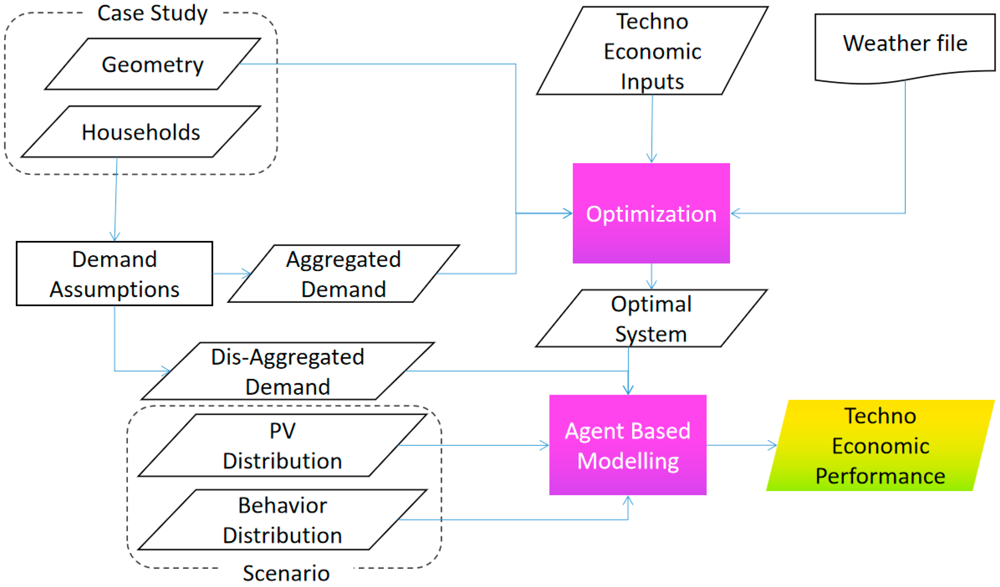
2. Research Methodology

This section will provide a brief introduction of the agent-based modelling algorithm used in terms of rules (which define behaviour of the agents), and different scenarios analysed (including various sets of PV distribution within the micro-grid and price schemes). After that, since the algorithm is applied on a case study, the case study will be described according to its features, how it is modelled, and the determination of the ideal PV system to be installed.

Figure 1 shows the workflow performed in this study, including the geometry of the building, the aggregated demand of the 48 households, a series of techno-economic inputs (see Table 4) and a local weather file. All these inputs are used to obtain the optimal PV system (i.e., the optimal capacity and positions for the modules in the system). After that, the optimal system is tested in a series of scenarios (see following section) using the agent-based modelling.

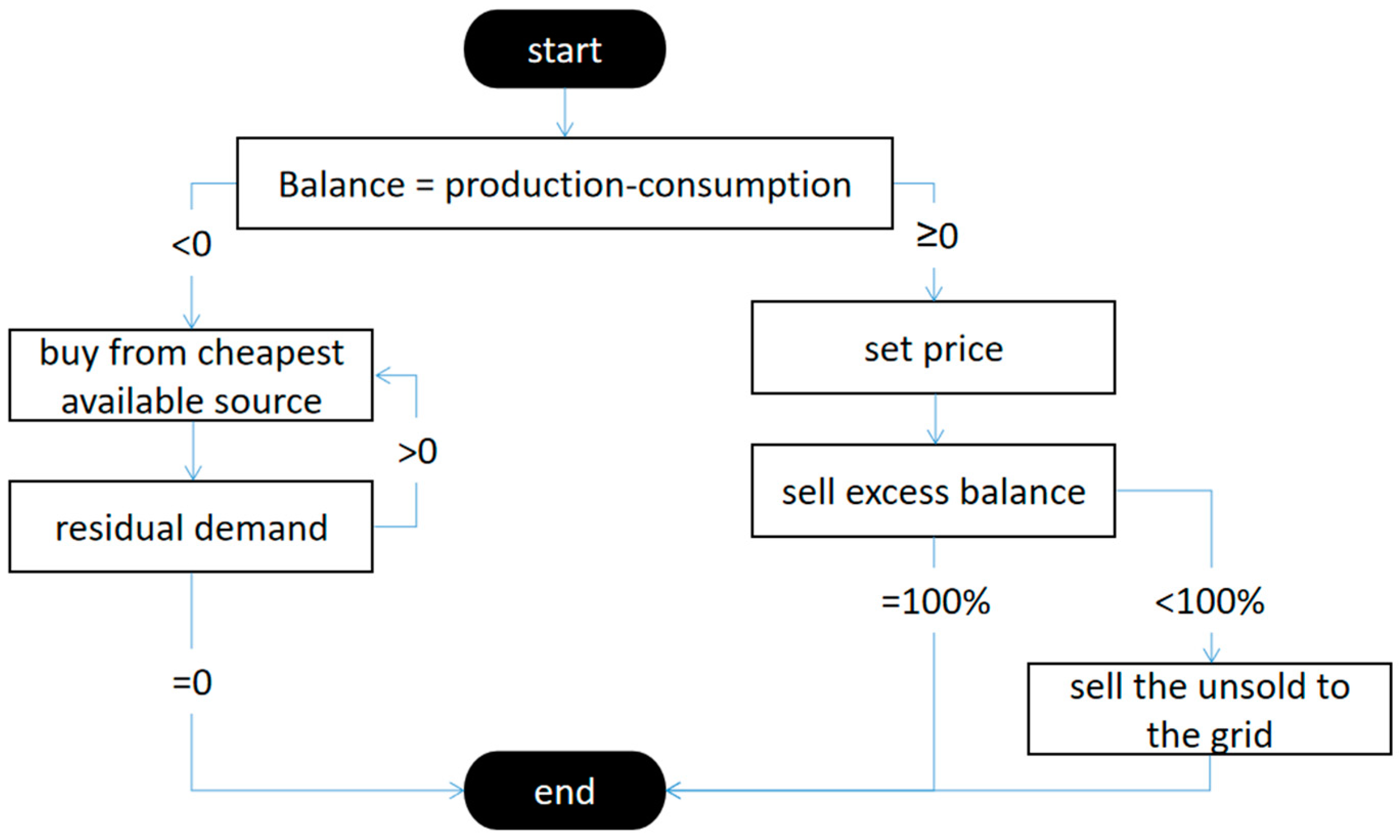
2.1. Agent Based Modelling and Scenarios

Occupant behaviour in buildings is complicated with different patterns and distribution properties [36,37,38]. An agent-based model is a model of a complex system where the behaviour is not controlled by a single algorithm, but it comes/emerges from the interaction of a number of sub-systems (i.e., the agents). Lovati et al. [39] proposed a 3D map of the possible algorithms (as shown in Figure 2); the dimensions represent the emergent versus controlled axis, the centralized versus decentralized axis, and the individual versus collective axis. The simulations presented in this study occupy the pink area in the map, and thus are individual, de-centralized systems causing an emergent behaviour in the micro-grid. In fact, in the scenarios described, there are multiple PV owners in the micro-grid and each one can set the price according to its own independent will.

It should be noted that, despite separate ownership, the agent-based model can be described by a simple set of rules:

• Every household is represented by one independent agent in the simulation.
• Every agent has an energy balance in each HOY (Hour of the Year). The energy balance is determined by its PV power (if it owns a PV system) minus its power demand in that particular HOY. If the balance is negative, the agent will be a net buyer in that HOY, otherwise it will be a seller. This rule implies that each agent can only sell electric power if it has already satisfied its own demand. Simply, each household can sell only excess PV production.
• Each seller can set the price for the power he has to export.
• If the electricity is offered by multiple sellers, the buying agent will buy preferentially from the cheapest source.
• If the aggregated demand of the district exceeds the offer of the cheapest source, the demand of each household is satisfied proportionally by the cheapest source. If, for example, the cheapest source covers 30% of the aggregated demand in that HOY, each household is provided 30% of its power demand by the cheapest source.
• If the on-site renewable power exceeds the power demand in a certain HOY, the cheapest sources are consumed preferentially, while the more expensive ones risk being in excess of the demand and sell part (or all) their power to the grid. Those who sell to the grid cannot set the price but are simply valued by the price paid by the grid (which is always way lower than that of the local sellers).

The same set of rules is applied on a set of six different scenarios; these are explained in the following paragraphs and summarized in

Table 1. PV capacities per household and prices in the 6 different scenarios.

Scenario	PV Capacity (kW/Household)	Electricity Price (at Year 0) (SEK/kWh)
(1)	1.36	1
(2)	1.36	1.19 (summer), 1.78 (winter)
(3)	2.73 or 0	1
(4)	2.73 or 0	1.19 (summer), 1.78 (winter)
(5)	1.36	1 or 1.19 (summer), 1.78 (winter)
(6)	1.36	1 or dynamic

.

Scenario 1: All residents agree to purchase the PV system; every household purchases an equal share of the total system and has thus the right to 1/48 of the power at any time (i.e., ca. 1.36 kW of capacity each). The price for the sale within the micro-grid is agreed for the long term as the summer grid price/1.2 (thus a static 1 SEK/kWh at the year 0); therefore, whoever buys electricity from another household saves ca. 17% on the electricity cost in summer and 45% in winter.

Scenario 2: All residents agree to purchase the PV system, like in Scenario 1. The price for the sale within the micro-grid is agreed for the long term as 99% of the grid price; therefore whoever buys electricity from another household has almost no savings compared to the grid. In this case it is assumed that using local energy is perceived as a value in itself by the participants in the grid.

Scenario 3: Only 50% of the residents agree to purchase the PV system; every PV equipped household purchases an equal share of the total system and has thus the right to 1/24 of the power at any time (i.e., ca. 2.73 kW each). The price for the sale within the micro-grid is agreed for the long term as the summer grid price/1.2, like in Scenario 1.

Scenario 4: Only 50% of the residents agree to purchase the PV system; every PV equipped household purchases an equal share of the total system like in Scenario 3. The price for the sale within the micro-grid is agreed for the long term as 99% of the grid price, like in Scenario 2.

Scenario 5: All residents agree to purchase the PV system, like in Scenario 1. The price for the sale within the micro-grid is left to the choice of the single household; 50% of the households decide to charge a high price (i.e., 99% of the grid, like case 2 and case 4), the others charge the summer price /1.2 like in Scenario 1 and Scenario 3.

Scenario 6: All residents agree to purchase the PV system. The price for the sale within the micro-grid is left to the choice of the single household like in Scenario 5, and 50% of the households decide to adopt a dynamic price system based on their energy balance in every hour of the year. With this strategy the energy is sold at LCOE whenever the balance is more than double the average balance in that hour of the day. The other 50% charges the 1 SEK per year like in Scenario 1 and Scenario 3.

In general, regardless of the scenario, the behavior of each agent in a time-step can be summarized as shown in Figure 3.

2.2. Modelling of the Economic Performance

To understand the profitability and the risks associated to the investment in the shared PV infrastructure the CAGR (Compound Annual Growth Rate) was used as key performance indicator. The CAGR has been considered in its real value i.e., without inflation, and expressed in percentual form according to the following equation:

$$\mathrm{CAGR}=\left[{\left(\frac{\mathrm{Inc}.-\left(\mathrm{CAPEX}+\mathrm{OPEX}\right)}{\mathrm{CAPEX}}\right)}^{\frac{1}{\mathrm{lifetime}}}-1\right]·100$$

(1)

In Equation (1), real Compound Annual Growth Rate is used to infer the profitability of the investment in the shared PV for each household.

• Inc. represents the cumulative income derived by the ownership of the share of the PV system during its lifetime; it represents the figure before costs (i.e., capital expenditure and operational expenditure) and it is calculated according to Equation (2).
• CAPEX is the capital expenditure; it includes the turn-key cost of the system including design and installation costs, but it assumes no taxation. It can be calculated by multiplying the unitary cost by the installed capacity (see Table 4).
• OPEX is the operational expenditure; it includes a standard annual cost of 80 SEK/kWp year for the substitution and cleaning of the modules, plus substitution of the inverter in case of rupture. The inverters have a cost of 3.5 KSEK/kWp and should be changed at least once in the planned lifetime of the system.
• Lifetime is expressed in years and is assumed as 30 years in this model.

$$\mathrm{Inc}.={\sum }_{\mathrm{T}=0}^{\mathrm{lifetime}}\left(\mathrm{Sav}.+\mathrm{Rev}.\right)·\left(1-\Delta \mathsf{\eta }·\mathrm{T}\right)·\left(1+\Delta \mathrm{d}·\mathrm{T}\right)$$

(2)

Equation (2): cumulative income derived by the ownership of the share of the PV system during its lifetime

• T represents the number of years since the construction of the PV system.
• Sav. Represents the savings due to the avoided purchase of electric power from the external grid, it is calculated according to Equation (3).
• Rev. Represents the revenues obtained by each shareholder by selling excess PV power from their share, it is calculated according to Equation (4).
• Δη is the variation of the efficiency due to ageing of the PV system. The shared PV is assumed to lose 1% per year (see Table 4).
• Δd is the variation in the price of the electricity for the consumer, it is assumed as +1.5% per year in design stage (see Table 4), but it is then assumed 0 or 2% in the agent based model (see Figure 8 in the results and Figure A1 in the Appendix A).

$$\mathrm{Sav}.={\sum }_{\mathrm{Ts}=1/1-00:30}^{31/12-23:30}\left(\left({\mathrm{P}}_{\mathrm{self},\mathrm{Ts}}·{\mathrm{d}}_{\mathrm{grid},\mathrm{Ts}}\right)+{\mathrm{P}}_{\mathrm{peer},\mathrm{Ts}}·\left({\mathrm{d}}_{\mathrm{grid},\mathrm{Ts}}-{\mathrm{d}}_{\mathrm{peer},\mathrm{Ts}}\right)\right)$$

(3)

Equation (3) savings due to the avoided purchase of electric power from the external grid.

• Ts represents the internal time-step of the model, in this case it is set as 1 h.
• P_self,Ts is the power self-consumed in a specific time-step.
• d_grid,Ts is the cost of electric power offered by the external grid in a specific time-step.
• P_peer,Ts is the power bought from a peer within the local community in a specific time-step.
• d_peer,TS is the cost of electric power offered by a peer in a specific time-step.

$$\mathrm{Rev}.={\sum }_{\mathrm{Ts}=1/1-00:30}^{31/12-23:30}\left(\left({\mathrm{P}\prime }_{\mathrm{peer},\mathrm{Ts}}·{\mathrm{d}\prime }_{\mathrm{peer},\mathrm{Ts}}\right)+\left({\mathrm{P}\prime }_{\mathrm{grid},\mathrm{Ts}}·{\mathrm{d}\prime }_{\mathrm{grid}}\right)\right)$$

(4)

Equation (4) revenues obtained by each shareholder by selling excess PV power from their share

• P′_peer,Ts is the power sold to all peers in a specific time-step
• d′_peer,Ts is the price set for selling power to the peers in a specific time-step
• P′_grid,Ts is the power sold to the grid in a specific time-step
• d′_grid is the price at which the grid purchases power. This price is static, thus is independent by the time-step.

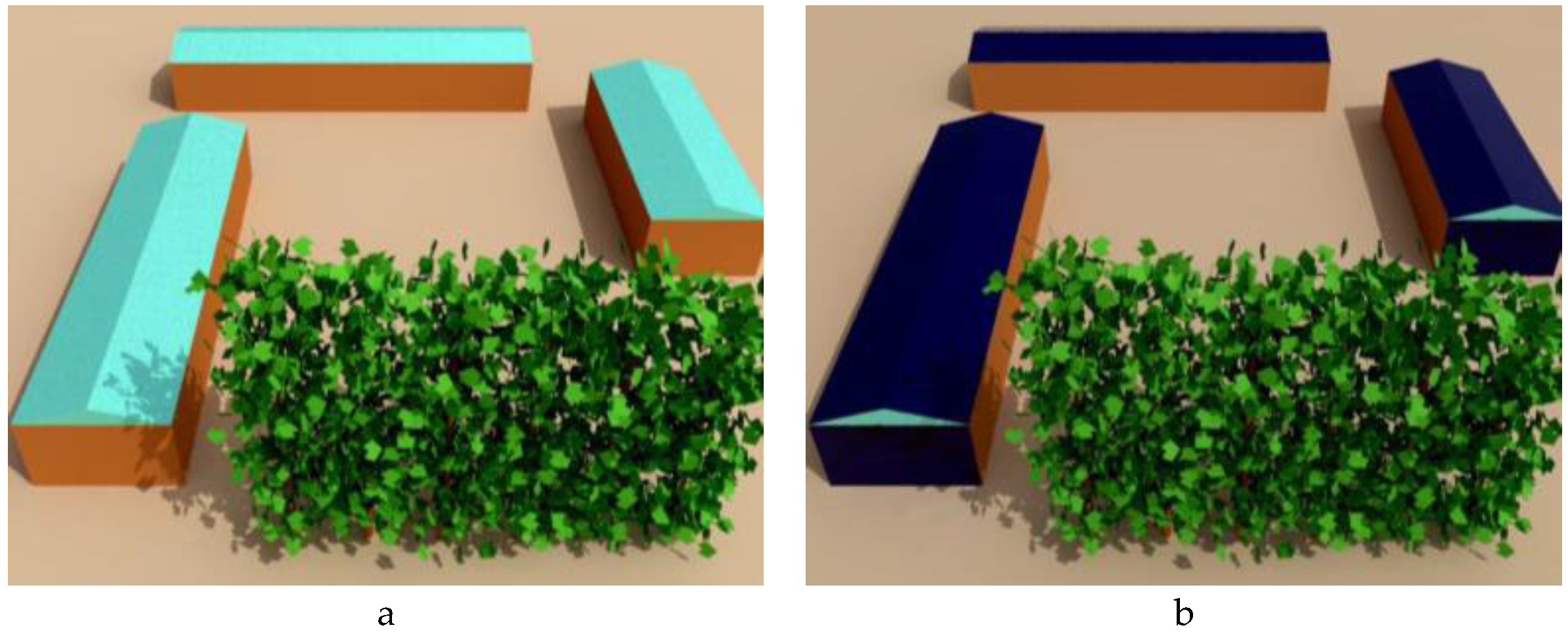
2.3. Case Study Description

A small district (or cluster) of residential buildings was adopted as a case study to test different behaviours of the co-owners (see Figure 4). The district is composed of three multi-family apartment blocks and it is located in Sunnansjö (Ludvika), in the Dalarna region of Sweden. The district is currently undergoing energy retrofit within the project Energy Matching [40] and is already the subject of scientific publication in [24,39,41]. While the geometric and technological properties of the site are known, the demographic information shall not be disclosed to respect the privacy of its inhabitants. For this reason, the electric demand used for the study was generated using LPG (Load Profile Generator) [42] assuming population characteristics as described in the following section (see Section 2.3). In total, there are 48 households in the three multi-family apartment blocks.

2.4. Electric Demand Assumptions

From previous study, the characteristic of electric demand with different spatial scales possesses various properties, and the aggregated electric use curves of more households indicate weaker randomness [43,44]. The composition of the district, made of 48 households, was assumed to reflect the demographic composition of Sweden as reported in the official statistics [45]. Due to the small sample of households, it was decided to curtail all the households listed in the ‘other’ category of the official data. These groups are difficult to transfer to a small sample because are numerically small, heterogeneous, and less specified than the main categories. For this reason, the district has been designed to match the main categories of household in Sweden (

Table 2. Number of persons and households in Sweden (excepts those listed in the ‘other’ category).

-	Male Minor	Female Minor	Male Adult	Female Adult	n Households
Single	0	0	921,495	957,910	1,879,405
Single + 1 minor	113,287	84,195	55,871	141,611	197,482
Single + 2 minor	108,963	96,493	25,907	76,821	102,728
Single + 3 minor	65,725	59,947	6146	30,676	36,822
Couple	0	0	1,134,261	1,132,893	1,132,893
Couple + 1 minor	208,795	169,207	377,046	378,958	377,046
Couple + 2 minor	494,165	453,061	472,734	474,492	472,734
Couple + 3 minor	340,621	309,381	194,487	194,905	194,487

) as shown in

Table 3. Number of persons and households in the district under exam as assumed to match the Swedish data [45].

-	Male Minor	Female Minor	Male Adult	Female Adult	n Households
Single	0	0	10	11	21
Single + 1 minor	2	1	1	2	3
Single + 2 minor	1	1	0	1	1
Single + 3 minor	0	0	0	0	0
Couple	0	0	12	12	12
Couple + 1 minor	2	2	4	4	4
Couple + 2 minor	5	5	5	5	5
Couple + 3 minor	3	3	2	2	2

. In the tables it is visible that the group ‘single + 3 kids’ has been removed as in proportion it amounts to almost zero households and would misrepresent the overall number of kids if one household was introduced.

Once the composition of the households was determined, the age and gender of the components have been estimated to match the data available online from the world factbook [46]. The resulting composition of the whole district have been reported in the Appendix A (see

Table A1. Composition by gender and age bracket of the inhabitants in the 48 HH (HouseHolds) in the district.

HH 1	HH 2	HH 3	HH 4	HH 5	HH 6	HH 7	HH 8
Male 25–54 Female 25–54 Male 0–14 Male 0–14 Female 0–14	Male 25–54 Female 25–54 Male 0–14 Female 0–14 Male 0–14	Male 25–54 Female 25–54 Female 0–14 Male 0–14	Male 25–54 Female 25–54 Female 0–14 Male 15–24	Male 25–54 Female 25–54 Female 15–24 Male 0–14	Male 25–54 Female 25–54 Female 0–14 Male 15–24	Male 25–54 Female 25–54 Female 15–24 Male 0–14	Male 25–54 Female 25–54 Female 0–14
HH 9	HH 10	HH 11	HH 12	HH 13	HH 14	HH 15	HH 16
Male 25–54 Female 25–54 Male 15–24	Male 25–54 Female 25–54 Female 15–24	Male 25–54 Female >65 Male 0–14	Female 25–54 Female 0–14 Male 15–24	Male >65 Female >65	Male >65 Female >65	Male >65 Female >65	Female 25–54 Male 0–14
HH 17	HH 18	HH 19	HH 20	HH 21	HH 22	HH 23	HH 24
Male 25–54 Female 0–14	Male 25–54 Female 25–54	Male 25–54 Female 15–24	Male 55–64 Female 25–54	Male >65 Female 55–64	Male 25–54 Female >65	Male 55–64 Female 25–54	Male >65 Female 55–64
HH 25	HH 26	HH 27	HH 28	HH 29	HH 30	HH 31	HH 32
Male 25–54 Female >65	Male 55–64 Female 25–54	Male >65 Female 55–64	Female >65	Male 25–54	Female 25–54	Male 55–64	Female 55–64
HH 33	HH 34	HH 35	HH 36	HH 37	HH 38	HH 39	HH 40
Male >65	Female >65	Male 25–54	Female 25–54	Male 55–64	Female 55–64	Male >65	Female >65
HH 41	HH 42	HH 43	HH 44	HH 45	HH 46	HH 47	HH 48
Male 15–24	Female 15–24	Male 25–54	Female 25–54	Male 55–64	Female 55–64	Male >65	Female >65

).

2.5. Calculation of the Optimal PV System

The optimal PV system, used in the micro-grid simulation, is the system that can maximize the self-sufficiency of the district while maintaining a positive NPV. The capacity and positions of such a PV system were found with the same technique and tool from the studies enumerated in the introduction (Section 1.3), which is one result of the H2020 project EnergyMatching. The parameters of the optimization are capacity and position of the PV system, if the capacity is too small the self-sufficiency will be low, but if the capacity is too high the overproduction of electricity will be too frequent, and the system will not be profitable. With the correct capacity (which leads to the largest profitable system) the self-sufficiency can be maximized; furthermore, installing parts of the PV system on the façade instead of on the roof can increase the contemporaneity between production and consumption [17]. In the case study described, considering the assumptions described in

Table 4. Assumption used in the optimization of the PV system.

Parameters	Values
Unitary cost of the PV system	12 KSEK/kWp (ca. 1175 €/kWp)
Unitary cost of electric storage	5.11 KSEK/kWh (ca. 500 €/kWh)
Planned lifetime of the system	30 years
Degradation of the PV system	−1%/year (annual percentual efficiency losses)
Nominal efficiency of the system	16.5%
Performance ratio of the system at standard test conditions	0.9
Price of the electricity from external grid	1.2 SEK/kWh (summer), 1.8 SEK/kWh (winter)
Price of the electricity sold to the external grid	0.3 SEK/kWh
Annual discount rate	3%
Growth of electric price for consumer	+1.5%/year (annual percentual price increases)

, the optimal system has a PV capacity of ca. 65.5 kWp, and no electric storage. The capacity on the southern slope of the roof (which is the most irradiated) is as high as it can be at 28.4 kWp, while part of the system has been installed on the southern façade (i.e., 5.3 kWp) despite large available spaces on the east and west slopes of the roof. The system can achieve an annual average self-sufficiency of ca. 24.6%. For the detailed design optimization of the PV systems, please refer to [24].

The optimization algorithm has a single target: its parameters are the capacity and positions of the PV system, and its reward function is the average annual self-sufficiency of the PV and building system. In the initial stage the building does not feature any PV system (capacity equals 0), then portions of PV area or electric storage are added or moved in an iterative procedure to maximize the reward function. Once it is not possible to further improve the function by adding or moving any component, the system is considered optimal and the algorithm ends.

The assumptions in Table 4 have been used for the dimensioning of the PV system according to the technique described in [17] and in numerous other studies mentioned in Section 1.3. The lifetime of the system is assumed at 30 years. However, the lifetime of the inverters is considered about 12.5 years and the expenses for its substitution are taken into account among maintenance costs (see [17]). The performance ratio of the system is considered 0.9. This value is not conservative as the average for urban installed systems is generally lower. Nevertheless, it should be considered that this is the performance ratio at standard test condition, which is therefore measured before temperature correction. Several examples in literature are considering the final performance ratio which is either measured experimentally or takes into account the temperature related losses. Several studies regarding urban photovoltaic systems, if controlled for calculated temperature-related losses, show values similar to 0.9 (see [47,48]). Significantly lower performance ratio at standard test condition could be expected in situations of strong partial shading. Furthermore, lower values can also arise in systems characterized by multiple facades if performance ratio is calculated measuring the irradiation in a single point, while production is calculated over the aggregated system. Nevertheless, these situations do not occur in the system under study. In term of efficiency, 16.5% was chosen; this value is conservative respect to the datasheets provided by numerous manufacturers. It should be noted that here, as in [17] and numerous studies mentioned in Section 1.3, the system does not represent the active area or the cumulative area of the modules, but the underlying area dedicated to the PV system. Since this a moderate sized rooftop system, and thus not equipped with empty passages for inspection, a utilization factor of the area of about 80% was assumed. This factor was taken into account by lowering the overall efficiency of the system.

3. Results and Discussion

After the simulation over an entire year in hourly time-step, all the exchanges of money and electric power that have happened in every time step between the different households are recorded in a ledger. The ledger is a Json archive; its size is large as it contains every interaction, both economic and of power, between a every single household with every other single household and the grid. Analysing this large file is possible in order to discover who has earned and who has lost in economic terms. Furthermore, it is possible to track the origin of the power that every household has consumed.

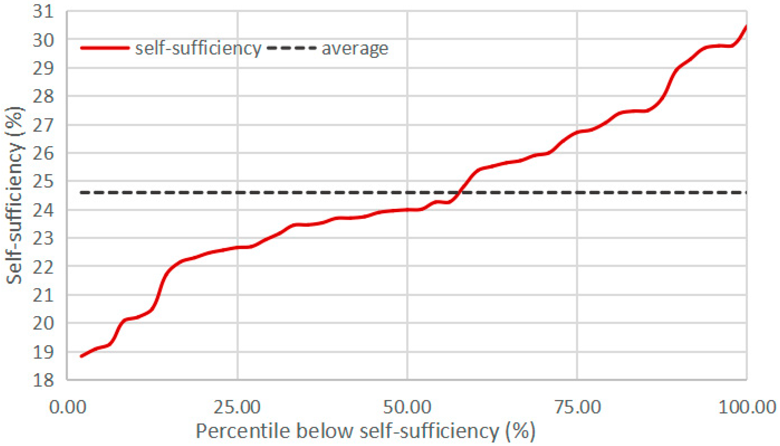
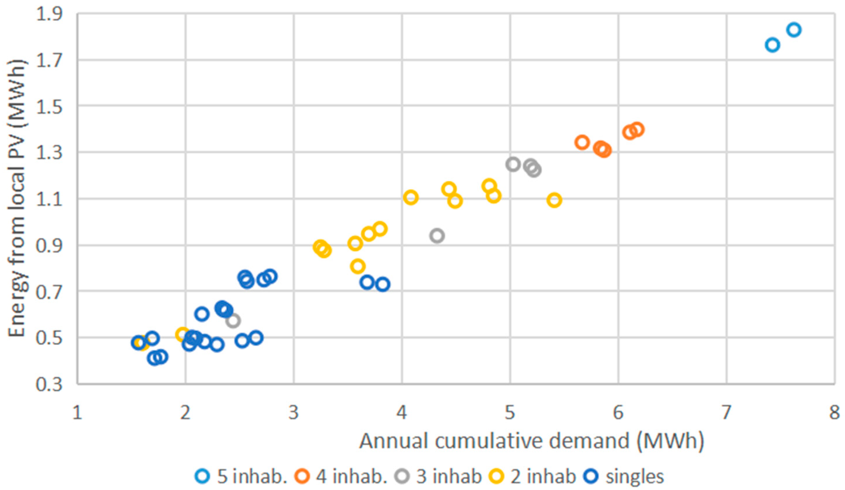
3.1. Self-Sufficiency within the Micro-Grid

Figure 5 shows the distribution of self-sufficiency throughout the district. Every point of the line describes the percentile of households that have a self-sufficiency lower than that described in the y-axis. It is visible, for example, that 90% of the district has a self-sufficiency lower than 29%. In other words, most of the district uses at least seventy percent of its energy from the grid. The flip side is that less than 10% of the households in the district has a self-sufficiency below 20%. This implies that the vast majority of households consumes at most 80% of their cumulative demand from non-local electricity. The result is notable because it far exceeds the solar fraction in the energy mix of even the best countries according to [49]. In general, the gradient of the curve seems to be slightly stronger at the extremes. It is rare to have an outlier with high or low self-sufficiency. In fact, about 70% of the households in the district fall within a variance of five percentage points of self-sufficiency (i.e., 22.5% and 27.5%).

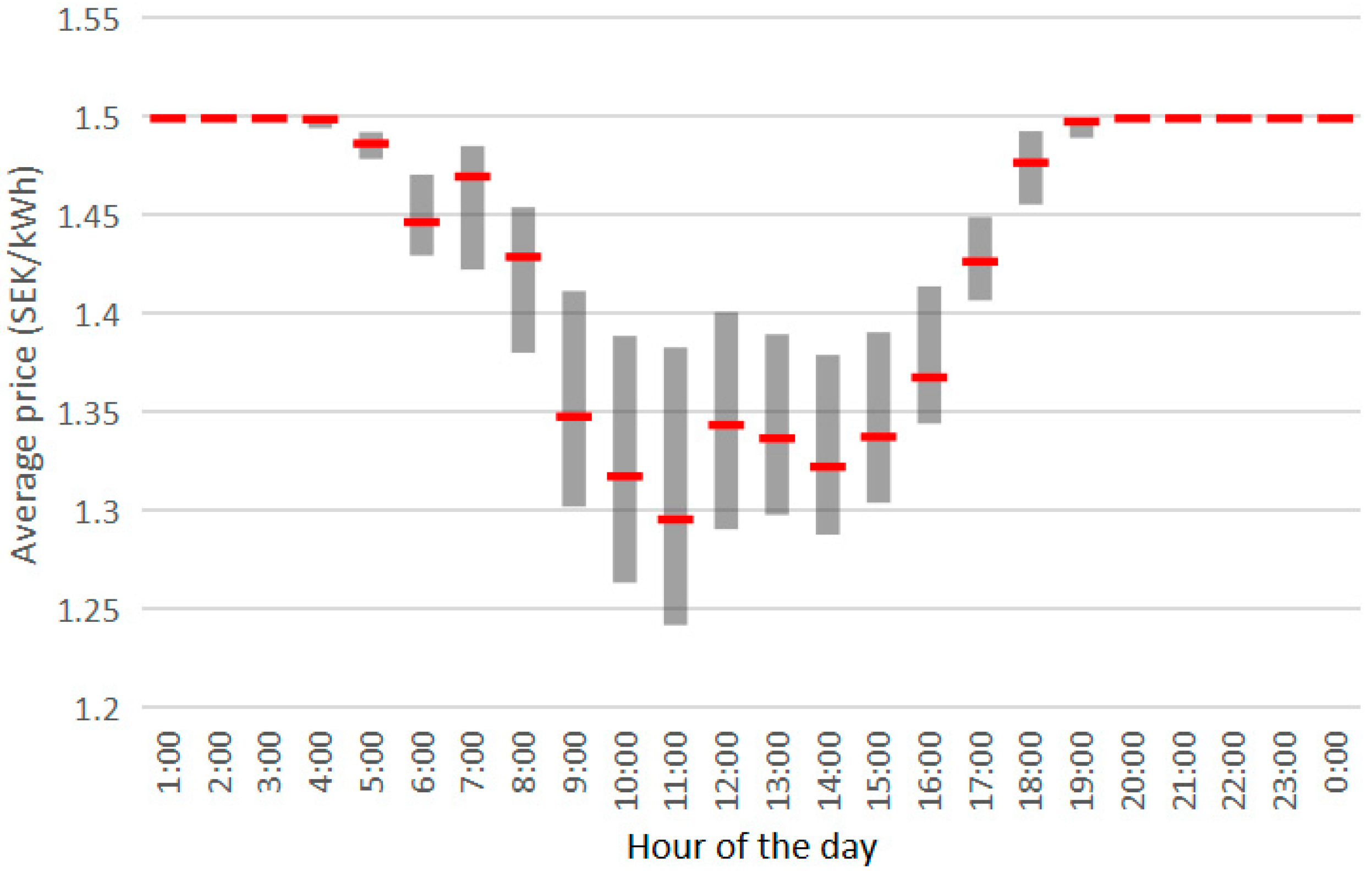
3.2. Effects of the Local Energy Market on the Price

Figure 6 describes the average hourly price for Scenario 1 during the different hours of the day within the district. The grey bands represent the variability between different households of the district. If a bar is longer, it means that some households have an average price that is significantly lower than others in that hour of the day. The red ticks represent the average price in that hour for the whole district. It is immediately visible that between 7 P.M. and 4 A.M. the price is almost stable at one point five SEK. The price is stable because there is no electric storage installed in the micro grid and, therefore, when a photovoltaic system is not producing, the price is that of the power provided by the electric grid. Considering that the night-time consumption of the district remains stable throughout the year, and that the electricity is sold at 1.8 SEK/kWh in winter and 1.2 SEK/kWh in summer, the night price paid by the whole district equals almost exactly the average of the two (i.e., 1.5 SEK/kWh). During daytime the price is lower; there are two reasons for this phenomenon. The first reason is that each household owns a share of the local PV system, and therefore all the electricity produced by their own share already belongs to them and is thus free for themselves. The second reason is that they can purchase electricity from their peers, the price of which is consistently lower than that of the grid. For these reasons, those households that are able to use larger share of their own electricity, or at least of the electricity from their peers, can enjoy a lower price for the electricity. It is visible, indeed expected, that the price of electricity is generally lower during the central hours of the day. Furthermore, it can be observed that times of the day of comparatively higher price correspond with moments of high electric demand. For example, it can be seen that the price is comparatively higher at seven and eight AM (when people prepare and consume breakfast) and at noon (when many prepare and consume lunch). This is due to the fact that, despite a large photovoltaic production in that hour, the outlier high demand forces the whole district to supply part of its demand from the external electric grid.

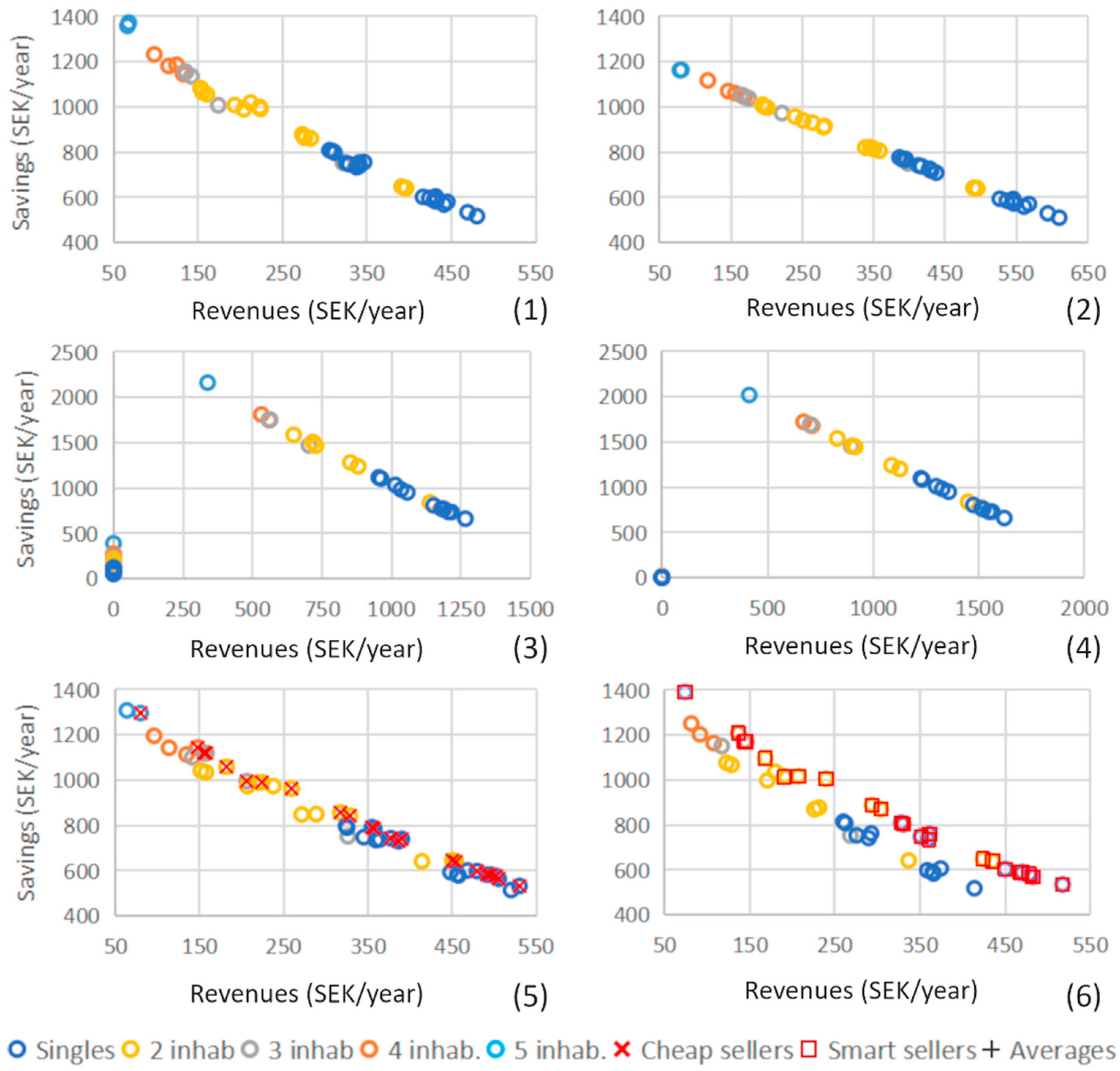
3.3. Savings and Revenues

Figure 7 shows the relationship between savings and revenues for each single household within the micro grid. All the sixth scenarios described previously are shown in the chart. In general, the savings are obtained either by using the electricity produced by one’s own system, therefore saving 100% of the price from the grid, or else by using the electricity from a peer household at a discounted price. On the other end the revenues are obtained either by selling electricity to the grid, or else by selling electricity to another household, the latter providing a much higher price. In each of the charts, every household is displayed as a circle, its position on the x-axis represents its annual revenues, while its position on the y-axis represents its annual savings. The colour of the circle line represents its belonging to a different category, according to the number of people living in the household. In general, these charts should be studied in their relative difference between each other, rather than in their absolute values. In fact, the absolute value of revenues and savings are not interesting when the cost of initial investment and those for the maintenance of the system are not taken into account. To see the lifetime techno-economic performance of the system, please check the next paragraph, which displays the CAGR. Observing the colour in all the cases it is visible that the smaller households (those which have a smaller electric demand) tend to show lower savings and higher revenues. This phenomenon is quite unsurprising because in the example considered every household purchases an equal capacity to all the others. Therefore, the small households will have a PV capacity that is larger relative to their demand, and will, thus, export and sell a larger fraction of the electricity that they produce.

3.4. Small Consumers Are ‘Sale Oriented’, Large Consumers Are ‘Savings Oriented’ (Scenario 1 vs. Scenario 2)

There is a noticeable difference between Scenario 1 and Scenario 2. In Scenario 1 every household agreed to sell their electricity at a significantly lower price compared to what they agree in Scenario 2 (see Table 1). Therefore, scenario one seems to be particularly advantageous for the largest consumers. This is due to the fact that the largest consumers have high savings but low revenues, and therefore, the sale of electricity at a lower price from others leads to higher savings for them, while it does not impact their revenues significantly. On the contrary, the smallest consumers, that have in general lower savings and higher revenues, will benefit from higher price of electricity. In this case, they will be able to increase their revenues greatly without changing their savings too much. In fact, being smaller, most of their savings comes from their own PV system, which is already over-dimensioned compared to their size. Going back to the largest consumers, a large fraction of their savings implies purchasing electricity from the smaller peers. Another noticeable aspect is that in Scenario 2, all the points are almost linearly correlated. This is due to the high price of the electricity sold, which is almost the same of the cost of electricity from the grid. The smaller remaining differences can be explained by the correlation between the private electric demand and the demand of the whole district. If a household over-produces electricity when the whole district is in over-production, its performances will be slightly lower because it will often sell to the grid. In the opposite case, when a household overproduces at times when there is need from other households, then its performance will be slightly higher.

3.5. When Some Agents Refuse to Invest in the Shared System, The Remaining Investors Have Larger Benefits and Lower Risks (Scenarios 3 and 4 vs. 1 and 2)

Scenarios 3 and 4 reflect Scenarios 1 and 2 in terms of price, but they have the peculiar aspect that only half of the households choose to purchase a PV system. This state of affairs would be very important for any practical application of the micro-grid. This is because, in practice, it is difficult to convince 100% of the tenants in a multi-family dwelling to participate, and especially to invest money, in a PV system. In a realistic setting it is expected that part of the population is unwilling to invest in the system; nevertheless, in the simulation it is assumed that they decided to participate in the micro-grid as simple consumers (i.e., those who do not own any part of the system). The assumption is safe because being a simple consumer only requires to always purchase the electricity from the cheapest source. In this way, to participate as a simple consumer does not have any initial cost nor risks, but it might have a benefit during the lifetime of the system. If Scenario 1 is compared to Scenario 3, it is visible that the points in the latter overwhelmingly outperform those in the former both in terms of revenues and in terms of savings. It is tolerably intuitive that, if only half of the households own a PV system, their revenues will increase. In fact, all the households who do not own PV can only buy the electricity from those who own it, and therefore, the whole local market moves in the direction of a “seller’s market”. Also, the increase in savings is readily explained. In fact, since the optimal capacity is unchanged in every scenario (see Section 2.4), every PV owner has at his disposal a larger capacity. This fact implies that there is more available electricity for self-consumption in every HOY, even at times of relatively high private electric demand. This spare over-capacity favours an increase in self-sufficiency. Looking at the bottom left corner of the chart for Scenario 3, it can be seen how there is a benefit in terms of savings also for those who do not own a PV system. Of course, these savings are minor compared to those of the other households, and this is due to two specific reasons. The first one is that, by lacking a PV system of their own, these households do not have their own electricity for free, and therefore can only purchase electricity from their peers. The second reason is that every household, before selling electricity, satisfies his own demand (see Section 2.1, in the rule b), and therefore those in the micro-grid who do not own a PV system can only benefit from the left-over electricity from the others. In other words, the household without PV can only purchase electricity when they happen to be in need of power at times when others are in overproduction. Scenario 4, like the Scenario 2, presents a linear correlation between the revenues and the savings of each household. Like Scenario 2 over Scenario 1, Scenario 4 also presents relatively higher revenues and lower savings compared to Scenario 3, thus favouring the smallest consumers. Furthermore, like Scenario 3, it presents a sharp contrast between the PV owners and the other households. It should be noted, though, that this time there is absolutely no benefit in participating in the micro-grid, or at least the benefits are so tiny that cannot be seen by the naked eye. There is nevertheless a benefit for those households: the possibility to increase the share of renewable on-site electricity in their energy consumption. It can be expected that, given the absence of initial investment, most consumers would be willing to increase their renewable energy share. By doing so, they have the possibility to save the planet with a costless, and thus effortless, action.

3.6. Interaction of Competing Sale Strategies within the Micro-Grid (Scenario 5 and Scenario 6)

In the first four scenarios, the price for the sale of PV power and the number of PV owners has been changed. Nevertheless, in all these cases, every PV owner agreed to maintain the same price as everybody else. In Scenario 5 the hypothesis is made that a half of the PV owners prefer to sell at the lower price (i.e., the price of the whole group of PV owners in Scenarios 2 and 4). Meanwhile the other half of the owners prefers to sell at the same price of Scenarios 1 and 3. Observing the revenues and the savings in this arrangement, it can be noted that, in general, the sellers who decide to sell for a lower price (‘cheap sellers’), enjoy a higher revenue compared to the others. Savings are not affected by the price of the sale of one’s own electricity, but rather by the price of available energy from the other households. For every savings level in the chart, the lowest selling households, which are marked as ‘cheap sellers’, appear to be on the right side compared to the others, which means that they have managed to obtain higher revenues. There are two factors at play when measuring the revenues in this type of market (where there are two different prices groups). The first factor is the sheer revenues per kWh sold; this acts by lowering the revenues for the so called ‘cheap sellers’. The second factor regards the ability to effectively sell your electricity within the micro grid at all. The capacity of not be in over supply, and thus forced to sell most of your power to the grid. If a different price was chosen, the result might have been different, but in this case the increased revenues derived from a higher price scheme are not enough to offset the increased instances in which the electricity cannot be sold due to high price and low demand. Also, in Scenario 6, the last one, the group of households was divided into two sub-groups. As in the previous scenario, some households were selling their electricity at a lower price compared to others. This time, though, the expensive sellers were given the ability to change the price according to a behaviour of their own. The mechanism used to change the price was set as explained in Scenario 6 of Section 2.1. In practice, these households, identified in the chart as ‘smart sellers’, will sell their power at the LCOE of the system, which is lower than the static price of the cheap sellers, whenever they have an outlier high energy balance in that specific hour of the day. In other words, when a smart seller has an outlier, low power consumption, or an outlier high power production from PV, it will sell its electric power at the lowest possible price. This strategy is extremely simple and is prone to numerous fallacies. In fact, if for example a particular household is on holiday during an unpopular period, its power demand would be unusually low, thus resulting in an outlier high balance. This could cause it to sell at LCOE in a time in which the electricity is indeed in high demand throughout the district. In this example, the household would be selling at the lowest possible price in a time in which the maximum price would still manage to sell to the peers. Conversely, if a household will experience an outlier high demand for its own reasons, it might find itself selling its available power dearly, while there might be plenty of energy available for everyone. It this case it will be forced to sell most its power to the electric grid. Despite the simplicity of this strategy and its obvious flaws, it is visible from the chart that such a simple behaviour is good enough for outsmarting the cheap sellers in the competition for the sale of electric power. Given any savings level, the smart sellers undeniably manage to obtain higher revenues. This is a very important result because it shows that it is possible to create an effective strategy without knowing the consumption of the other agents in the micro grid, thus avoiding privacy issues.

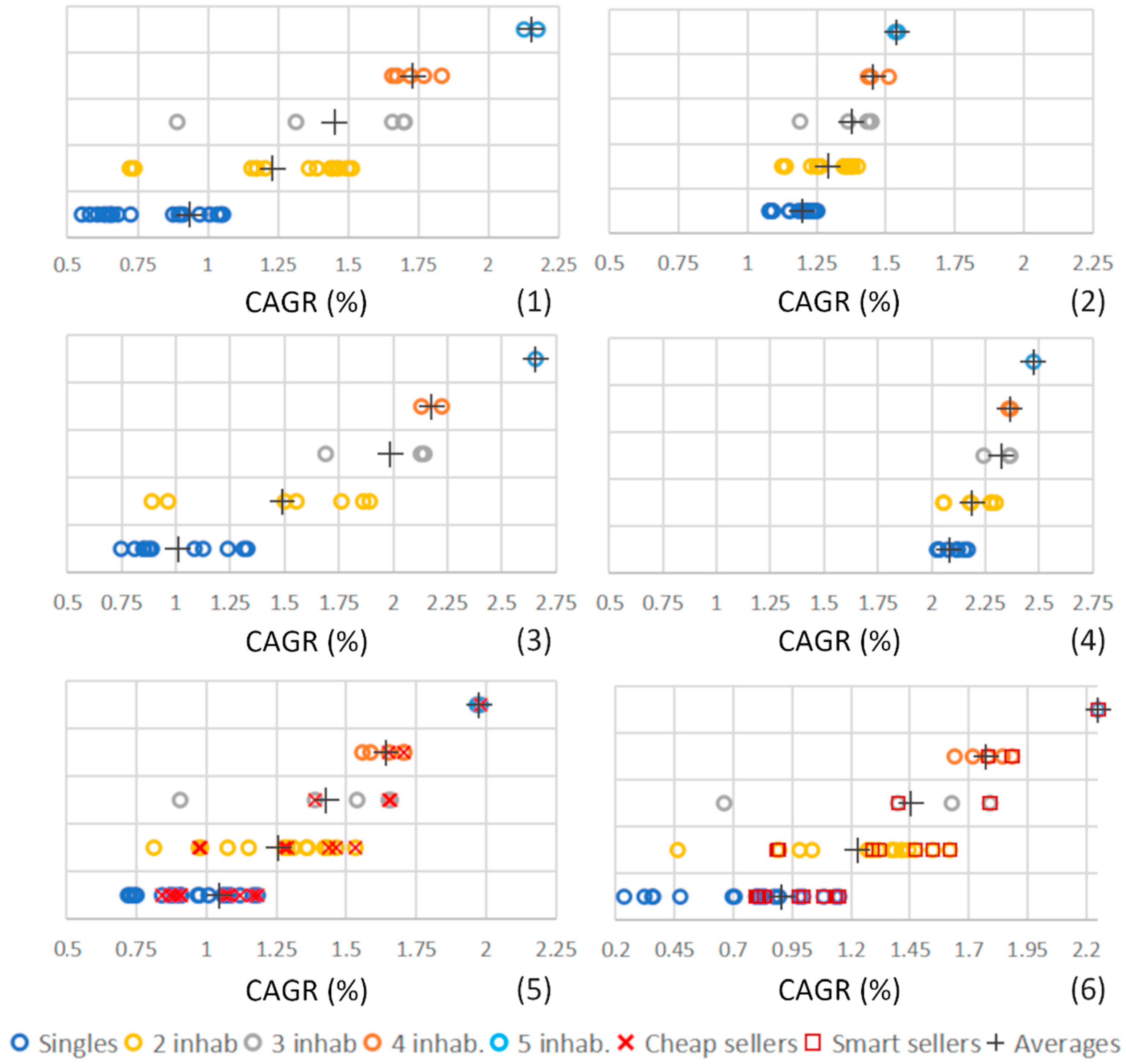
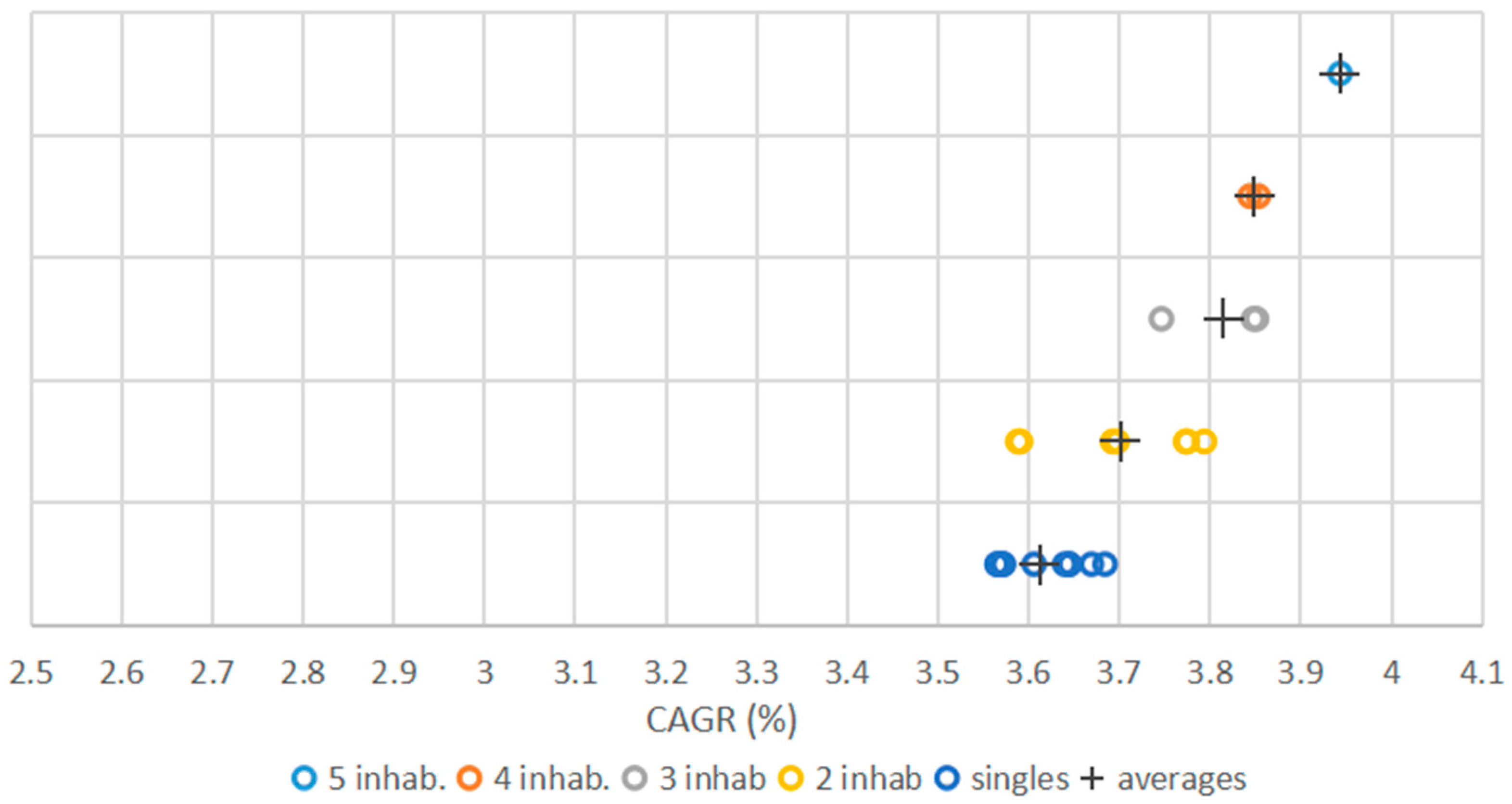
3.7. Effects of the Phenomenon Observed on the Cagr (Compound Annual Growth Rate) for Every Household

Figure 8 represents the real CAGR for the PV owners in the micro-grid; as in the previous set of charts, every circle represents one household.

This time no information is provided on the ‘y’ axes; the households are simply divided into groups to enhance the readability of the chart. The black crosses represent the average CAGR of each group (according to the number of inhabitants in the household). At first glance these CAGR might look low, but it should be noted that they are produced with two strongly conservative assumptions: the CAGR is real (note it does not consider inflation over a period of 30 years) and the price of electricity for the consumer is considered stable throughout the lifetime of the system (which means it will not grow despite the large investments needed to renew the grid infrastructure and potential future carbon taxation). Some examples of real CAGR considering a 2% linear price growth for the household electricity can be found in Appendix A. In general, it can be seen that larger households, those with higher number of inhabitants and higher electric demand, fare better than the smaller ones in terms of CAGR. This fact must be due to larger households being able to exploit the savings derived by their own PV system more often, and more often benefit from purchasing energy from their peers. Looking at the difference between Scenarios 1 and 2, it is visible how the relative difference in average CAGR between groups is lower in Scenario 2. This means that larger households benefit more from internal sale of electricity compared to smaller ones. This fact is quite intuitive since every household owns an equally sized PV system, and thus having a larger electric demand increases the frequency of over-consumption with respect to one’s own electricity. In Scenario 2, where the benefit of buying from peers has been almost completely removed, there is a residual advantage in being a large consumer. This is due to the higher self-consumption of the large consumers. In fact, having a large self-consumption of one’s own electricity reduces the risk of not having buyers in a specific HOY; it does so by reducing the very number of hours in which one needs a buyer. Furthermore, though negligible, in case 2 there is also the 1% difference in price between the external and the internal electricity. Scenarios 3 and 4 reflect Scenarios 1 and 2 except that only 50% of the households decide to install PV, and thus are entitled to twice the capacity of before. In Scenario 3 and 4 the CAGR of every group are sensibly increased compared to the respective Scenarios 1 and 2. This at first might sound counter-intuitive for Scenario 3 (i.e., electricity sold for cheap) considering the lower self-consumption given by a larger per capita system. Nevertheless, even though the instances of over-production are more frequent for PV owners, there is a larger number of buyers among the peers because half of the households do not own a PV system, and the price of sale, though low, is still higher than the LCOE of the system. Furthermore, even though self-consumption is lowered by a larger system, self-sufficiency is increased and allows for higher savings from avoided electricity consumption. In other words, having a larger system increases the savings of the owners, and being in a ‘seller’s market’ due to the lower proportion of PV owners, the risk of selling to the grid is also reduced. This explains the sensible increase of CAGR from Scenario 1 to Scenario 3, and the massive increase from Scenario 2 to Scenario 4. In terms of CAGR, Scenario 5 and Scenario 6 reinforce the signal obtained previously in terms of revenues. In fact, in Scenario 5 (when part of the households sells at generally at a lower price) the so called ‘cheap sellers’ drive the others outside of the market forcing them to sell a large fraction of their electricity to the grid. This is visible by the fact that the cheap sellers consistently occupy the right side of the dispersion in every group (i.e., achieve higher CAGR for every group). Conversely, when the expensive sellers are given the ability to modulate the price according to their own energy balance, despite the simple and flawed nature of the algorithm, they secure the rightmost side of the dispersion in the different groups.

4. Conclusions

4.1. Key Findings

Several previous studies have demonstrated that urban PV systems can be economically feasible while covering a large portion of the residential electric demand (i.e., more than 20% or even 30%); this can be achieved in large parts of Europe without incentives and without necessarily adding any electric storage. It has also been found that the aggregation of the demand strongly increases the optimal capacity of PV, regardless of the reward function used for the optimization.

The optimal design of the PV system does not address the problem of financing and distribution of the risks and benefits of the system, especially if it is shared between multiple owners (which is the most promising case to ramp up urban PV capacity). For this reason, an agent-based modelling environment has been developed. The environment is capable of simulating potential PV production, electric demand, and price setting for each household independently and recording their interactions. The behaviour and PV distribution of the agents has been varied in six different scenarios in which the agents have been free to interact. The annual average self-sufficiency of the whole district reaches 24+%, this is remarkably considering the latitude and the absence of incentives and electric storage.

In general, smaller households (with less components and a lower annual cumulative demand) are characterized by higher revenues and lower savings compared to larger households (see Figure 7); this is due to having a larger system comparative to their size and, thus, a frequent over-production of electricity. The smaller household, being more ‘sale oriented’ benefitted from scenarios in which the price schemes in the micro-grid were high (see Figure 8 (2) and (4) against (1) and (3)). It seems, therefore, that high prices of the electricity within the micro-grid favour a more equal distribution of the risks and benefits. That said, being the households free to choose their price, they are unlikely to move toward a very high price, which is almost the same as the grid. Even more so, because the lowering of the price appears to be the simplest effective strategy to increase the CAGR (see in Figure 8 (5)).

Considering a real case study, it is very likely that some of the households in a micro-grid (which could be located in a multi-family building or a district) would absolutely refuse to invest money in the shared PV system. Simulating this hypothesis in two scenarios (i.e., 3 and 4) showed increases in both revenues and savings for every group (see Figure 7 (3) against (1), and (4) against (2)). This, unsurprisingly, resulted in improved CAGR for those who own a PV system (see Figure 8 (3) against (1), and (4) against (2)). This result is fortunate in the sense that incentives to invest are automatically generated whenever somebody is unwilling to participate in the investment. In this sense, Scenario 4 is a particularly promising one because a limited fraction of the households could form a consortium and provide renewable electricity at the same price of the one offered by the external grid. This could allow the investor to have safe and interesting CAGR (see case 4 assuming a price growth of 2% in the Appendix A), while the non-investors, albeit without any economic advantage, could increase their renewable use without costs nor risks.

In the last scenario it was hypothesized that part of the households, to out-compete the ‘cheap sellers’, would adopt a dynamic price scheme based on their own energy balance. In practice, they would sell their excess power at a very low price whenever their balance was above average (compared to that hour of the day). Conversely, they would sell their power at the highest possible price whenever their balance is below the average of that hour. This strategy, despite its simplicity, and despite being unaware of the actual balance of the other households, is shown to easily out-compete the ‘cheap sellers’. This is remarkable as it proves that effective strategies are possible without invading other household’s privacy, but are solely based on data relative to oneself.

4.2. Future Work

The findings from this technique inevitably lead to new questions; in particular, there are four aspects that should be investigated more deeply:

• It has been shown that reducing the number of PV owners (leaving unchanged the aggregated PV capacity, which is the optimal one) boosts the CAGRs for those who remain. Nevertheless, this has been done only in two scenarios, in which the percentage of owners was invariably 50% instead of 100%. It would be useful to explore an array of different percentages of PV owners combined in different price schemes, thus understanding the phenomenon more thoroughly. Being a very encouraging aspect of the micro-grid, this advantage of the ‘rare owners’ might be hiding some effective business models.
• One feature of this local energy market is represented by rule ‘e’ from Section 2.1. This rule commands that, in the case of insufficient supply of the cheapest source, the power from the cheapest source should be provided proportionally to every agent’s demand. Given the disadvantage experienced by smallest consumers, especially when the overall price of the electricity is low, it would be interesting to explore what happens with a different rule. For example, it would be interesting to provide each agent with equal power instead of satisfying the same proportion. With this difference, having a low consumption would actually boost the self-sufficiency considerably, and perhaps lead to a more balanced share of benefits and risks.
• The dynamic pricing behaviour with which half of the agents were endowed in Scenario 6 demonstrates the effectiveness of a simple dynamic pricing strategy. While only a proof of concept, this strategy is the first step in exploring a large array of behaviors that the agents could assume. It would be interesting to explore the impact of machine learning driven behaviours varying in complexity and in inputs required (both historical and real-time) [50].
• This study focuses on economic sustainability and fairness of different ownership and pricing schemes. Thus, it assumes the regulatory aspects as capable to allow a fruitful market structure. However, the regulatory design will be essential to achieve such local market, such as metering, and billing/collection, as well as responsibility allocation etc.
• The results of this study are obtained in a purely residential district; nevertheless, the presence of commercial, office, or public buildings would increase the contemporaneity of production and load. This effect would generally improve the techno-economic performance of the whole system; this improvement should be quantified to allow for spatial planning of the electric infrastructure.

References

1. Lovelock, C.E.; Reef, R. Variable Impacts of Climate Change on Blue Carbon. One Earth 2020, 3, 195–211. [Google Scholar] [CrossRef]
2. Zhou, P.; Wang, G.; Duan, R. Impacts of long-term climate change on the groundwater flow dynamics in a regional groundwater system: Case modeling study in Alashan, China. J. Hydrol. 2020, 590, 125557. [Google Scholar] [CrossRef]
3. Jiang, Q.; Qi, Z.; Tang, F.; Xue, L.; Bukovsky, M. Modeling climate change impact on streamflow as affected by snowmelt in Nicolet River Watershed, Quebec. Comput. Electron. Agric. 2020, 178, 105756. [Google Scholar] [CrossRef]
4. Huang, M.; Ding, L.; Wang, J.; Ding, C.; Tao, J. The impacts of climate change on fish growth: A summary of conducted studies and current knowledge. Ecol. Indic. 2021, 121, 106976. [Google Scholar] [CrossRef]
5. Leisner, C.P. Review: Climate change impacts on food security- focus on perennial cropping systems and nutritional value. Plant Sci. 2020, 293, 110412. [Google Scholar] [CrossRef] [PubMed]
6. He, Q.; Silliman, B.R. Climate Change, Human Impacts, and Coastal Ecosystems in the Anthropocene. Curr. Biol. 2019, 29, R1021–R1035. [Google Scholar] [CrossRef]
7. Guo, S.; Yan, D.; Hu, S.; An, J. Global comparison of building energy use data within the context of climate change. Energy Build. 2020, 226, 110362. [Google Scholar] [CrossRef]
8. Liu, W.; McKibbin, W.J.; Morris, A.C.; Wilcoxen, P.J. Global economic and environmental outcomes of the Paris Agreement. Energy Econ. 2020, 90, 104838. [Google Scholar] [CrossRef]
9. Giddens, A. The Constitution of Society: Outline of the Theory of Structuration; University of California Press: Oakland, CA, USA, 1984. [Google Scholar]
10. Geels, F.W.; Schot, J. Typology of sociotechnical transition pathways. Res. Policy 2007, 36, 399–417. [Google Scholar] [CrossRef]
11. Geels, F.W. Technological transitions as evolutionary reconfiguration processes: A multi-level perspective and a case-study. Res. Policy 2002, 31, 1257–1274. [Google Scholar] [CrossRef] [Green Version]
12. Suarez, F.F.; Oliva, R. Environmental change and organizational transformation. Ind. Corp. Chang. 2005, 14, 1017–1041. [Google Scholar] [CrossRef] [Green Version]
13. Scott, W.R. Institutions and Organizations: Ideas, Interests, and Identities; Sage Publications: Thousand Oaks, CA, USA, 2013. [Google Scholar]
14. Smith, A.; Stirling, A.; Berkhout, F. The governance of sustainable socio-technical transitions. Res. Policy 2005, 34, 1491–1510. [Google Scholar] [CrossRef]
15. Bigerna, S.; Bollino, C.A.; Micheli, S.; Polinori, P. A new unified approach to evaluate economic acceptance towards main green technologies using the meta-analysis. J. Clean. Prod. 2017, 167, 1251–1262. [Google Scholar] [CrossRef]
16. Atalla, T.; Bigerna, S.; Bollino, C.A.; Polinori, P. An alternative assessment of global climate policies. J. Policy Modeling 2018, 40, 1272–1289. [Google Scholar] [CrossRef]
17. Lovati, M.; Salvalai, G.; Fratus, G.; Maturi, L.; Albatici, R.; Moser, D. New method for the early design of BIPV with electric storage: A case study in northern Italy. Sustain. Cities Soc. 2019, 48, 101400. [Google Scholar] [CrossRef] [Green Version]
18. Huang, P.; Sun, Y.; Lovati, M.; Zhang, X. Solar-photovoltaic-power-sharing-based design optimization of distributed energy storage systems for performance improvements. Energy 2021, 222, 119931. [Google Scholar] [CrossRef]
19. Huang, P.; Zhang, X.; Copertaro, B.; Saini, P.K.; Yan, D.; Wu, Y.; Chen, X. A Technical Review of Modeling Techniques for Urban Solar Mobility: Solar to Buildings, Vehicles, and Storage (S2BVS). Sustainability 2020, 12, 7035. [Google Scholar] [CrossRef]
20. Adami, J.; Lovati, M.; Maturi, L.; Moser, D. Evaluation of the impact of multiple PV technologies integrated on roofs and façades as an improvement to a BIPV optimization tool. In Proceedings of the 14th Conference on Advanced Building Skins, Bern, Switzerland, 28–29 October 2021. [Google Scholar]
21. Vigna, I.; Lovati, M.; Pernetti, R. A modelling approach for maximizing RES harvesting at building cluster scale. In Proceedings of the 4th Building Simulation and Optimization Conference, Cambridge, UK, 11–12 September 2018. [Google Scholar]
22. Lovati, M.; Adami, J.; Dallapiccola, M.; Maturi, L.; Moser, D. From Solitary Pro-Sumers to Energy Community: Quantitative Assesment of the Benefits of Sharing Electricity. IEEE Trans. Power Syst. 2019. [Google Scholar] [CrossRef]
23. Fina, B.; Auer, H.; Friedl, W. Profitability of PV sharing in energy communities: Use cases for different settlement patterns. Energy 2019, 189, 116148. [Google Scholar] [CrossRef]
24. Huang, P.; Lovati, M.; Zhang, X.; Bales, C.; Hallbeck, S.; Becker, A.; Bergqvist, H.; Hedberg, J.; Maturi, L. Transforming a residential building cluster into electricity prosumers in Sweden: Optimal design of a coupled PV-heat pump-thermal storage-electric vehicle system. Appl. Energy 2019, 255, 113864. [Google Scholar] [CrossRef]
25. Lovati, M.; Dallapiccola, M.; Adami, J.; Bonato, P.; Zhang, X.; Moser, D. Design of a residential photovoltaic system: The impact of the demand profile and the normative framework. Renew. Energy 2020, 160, 1458–1467. [Google Scholar] [CrossRef]
26. Gjorgievski, V.Z.; Cundeva, S.; Georghiou, G.E. Social arrangements, technical designs and impacts of energy communities: A review. Renew. Energy 2021, 169, 1138–1156. [Google Scholar] [CrossRef]
27. Caramizaru, A.; Uihlein, A. Energy Communities: An Overview of Energy and Social Innovation; Publications Office of the European Union: Luxembourg, 2020. [Google Scholar]
28. Capellán-Pérez, I.; Johanisova, N.; Young, J.; Kunze, C. Is community energy really non-existent in post-socialist Europe? Examining recent trends in 16 countries. Energy Res. Soc. Sci. 2020, 61, 101348. [Google Scholar] [CrossRef] [Green Version]
29. Lowitzsch, J.; Hoicka, C.E.; van Tulder, F.J. Renewable energy communities under the 2019 European Clean Energy Package—Governance model for the energy clusters of the future? Renew. Sustain. Energy Rev. 2020, 122, 109489. [Google Scholar] [CrossRef]
30. Moroni, S.; Alberti, V.; Antoniucci, V.; Bisello, A. Energy communities in the transition to a low-carbon future: A taxonomical approach and some policy dilemmas. J. Environ. Manag. 2019, 236, 45–53. [Google Scholar] [CrossRef]
31. Roberts, M.B.; Bruce, A.; MacGill, I.J.S.E. A comparison of arrangements for increasing self-consumption and maximising the value of distributed photovoltaics on apartment buildings. Sol. Energy 2019, 193, 372–386. [Google Scholar] [CrossRef]
32. Novoa, L.; Flores, R.; Brouwer, J. Optimal renewable generation and battery storage sizing and siting considering local transformer limits. Appl. Energy 2019, 256, 113926. [Google Scholar] [CrossRef]
33. Abada, I.; Ehrenmann, A.; Lambin, X. On the viability of energy communities. Energy J. 2020, 41. [Google Scholar] [CrossRef]
34. Sadeghian, H.; Wang, Z. A novel impact-assessment framework for distributed PV installations in low-voltage secondary networks. Renew. Energy 2020, 147, 2179–2194. [Google Scholar] [CrossRef]
35. Awad, H.; Gül, M. Optimisation of community shared solar application in energy efficient communities. Sustain. Cities Soc. 2018, 43, 221–237. [Google Scholar] [CrossRef]
36. Qian, M.; Yan, D.; Liu, H.; Berardi, U.; Liu, Y. Power consumption and energy efficiency of VRF system based on large scale monitoring virtual sensors. Build. Simul. 2020, 13, 1145–1156. [Google Scholar] [CrossRef]
37. Hu, S.; Yan, D.; Guo, S.; Cui, Y.; Dong, B. A survey on energy consumption and energy usage behavior of households and residential building in urban China. Energy Build. 2017, 148, 366–378. [Google Scholar] [CrossRef]
38. Jin, Y.; Xu, J.; Sun, H.; An, J.; Tang, J.; Zhang, R. Appliance use behavior modelling and evaluation in residential buildings: A case study of television energy use. Build. Simul. 2018, 13, 787–801. [Google Scholar] [CrossRef]
39. Lovati, M.; Zhang, X.; Huang, P.; Olsmats, C.; Maturi, L. Optimal Simulation of Three Peer to Peer (P2P) Business Models for Individual PV Prosumers in a Local Electricity Market Using Agent-Based Modelling. Buildings 2020, 10, 138. [Google Scholar] [CrossRef]
40. EnergyMatching. European Union’s Horizon 2020 Research and Innovation Programme under Grant Agreement Nº 768766. Available online: https://www.energymatching.eu/project/ (accessed on 20 October 2020).
41. Huang, P.; Lovati, M.; Zhang, X.; Bales, C. A coordinated control to improve performance for a building cluster with energy storage, electric vehicles, and energy sharing considered. Appl. Energy 2020, 268, 114983. [Google Scholar] [CrossRef]
42. Pflugradt, N.; Muntwyler, U. Synthesizing residential load profiles using behavior simulation. Energy Procedia 2017, 122, 655–660. [Google Scholar] [CrossRef]
43. Xu, J.; Kang, X.; Chen, Z.; Yan, D.; Guo, S.; Jin, Y.; Hao, T.; Jia, R. Clustering-based probability distribution model for monthly residential building electricity consumption analysis. Build. Simul. 2021, 14, 149–164. [Google Scholar] [CrossRef]
44. Fan, C.; Yan, D.; Xiao, F.; Li, A.; An, J.; Kang, X. Advanced data analytics for enhancing building performances: From data-driven to big data-driven approaches. Build. Simul. 2021, 14, 3–24. [Google Scholar] [CrossRef]
45. Statistics Sweden. Sveriges Officiella Statistik: Personer Efter Hushållstyp, Hushållsställning och kön 31 December 2019 (Excel File). Available online: https://www.scb.se/hitta-statistik/statistik-efter-amne/befolkning/befolkningens-sammansattning/befolkningsstatistik#_Tabellerochdiagram (accessed on 20 October 2020).
46. Central Intelligence Agency. The World Factbook. 2020. Available online: https://www.cia.gov/library/publications/resources/the-world-factbook/index.html (accessed on 16 November 2020).
47. Imenes, A.G. Performance of BIPV and BAPV Installations in Norway. In Proceedings of the IEEE 43rd Photovoltaic Specialists Conference (PVSC), Portland, OR, USA, 5–10 June 2016; pp. 3147–3152. [Google Scholar]
48. López, C.S.P.; Frontini, F.; Friesen, G.; Friesen, T.J.E.P. Experimental testing under real conditions of different solar building skins when using multifunctional BIPV systems. Energy Procedia 2014, 48, 1412–1418. [Google Scholar] [CrossRef] [Green Version]
49. Masson, G.; Kaizuka, I.; Detolleanere, A.; Lindahl, J.; Jäger-Waldau, A. 2019–Snapshot of Global Photovoltaic Markets; IEA International Energy Agency: Paris, France, 2019. [Google Scholar]
50. Hu, S.; Yan, D.; Azar, E.; Guo, F. A systematic review of occupant behavior in building energy policy. Build. Environ. 2020, 175, 106807. [Google Scholar] [CrossRef]
51. Zhang, C.; Wu, J.; Long, C.; Cheng, M.J.E.P. Review of existing peer-to-peer energy trading projects. Energy Procedia 2017, 105, 2563–2568. [Google Scholar] [CrossRef]
Figure 1. Flow diagram of the data and operations performed for this study.
Buildings 11 00160 g001
Figure 2. 3D map of the behaviours in a district scale renewable energy system from [39].
Buildings 11 00160 g002
Figure 3. Schematic of the behaviour of each agent in every time-step of the simulation.
Buildings 11 00160 g003
Figure 4. View of the (a) 3D model used to calculate PV production in the district and (b) areas that is possible to dedicate to PV highlighted. The model represents the three multi-family buildings that comprise the 48 households in the study. Please note that each household does not own any physical portion of the roof as it is commonly owned. If a household decides to invest in the shared PV system, it becomes shareholder of the common infrastructure (it does not purchase a physical small system on the roof).
Buildings 11 00160 g004
Figure 5. Self-sufficiency within the micro-grid.
Buildings 11 00160 g005
Figure 6. Average price for each hour of the day and its variability within the district (Scenario 1).
Buildings 11 00160 g006
Figure 7. Savings V.S. revenues for each household in the microgrid. Both axes are in SEK/year (1) Scenario 1 (2) Scenario 2 (3) Scenario 3 (4) Scenario 4 (5) Scenario 5 (6) Scenario 6.
Buildings 11 00160 g007
Figure 8. CAGR (Compound Annual Growth Rate) % in the different scenarios (16), the CAGR are real (i.e., would be higher if adjusted for inflation), and assume a case in which there is no growth in the price of electricity, a chart assuming a 2% linear increase in the price of electricity from Scenario 4 is in the Appendix A.
Buildings 11 00160 g008