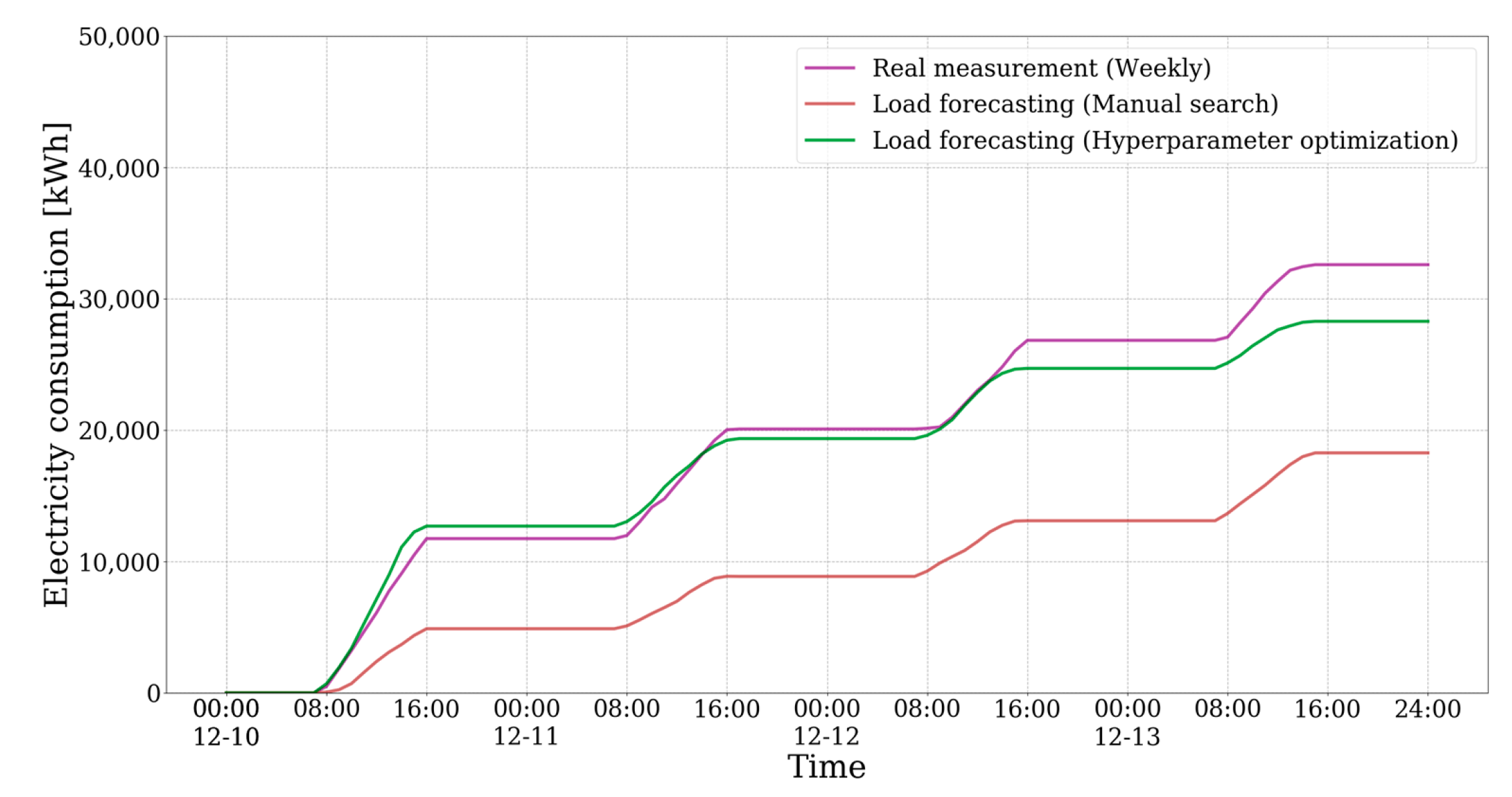
Article

Development and Validation of Building Control Algorithm Energy Management

School of Mechanical Engineering, Chonnam National University, Gwangju 61186, Korea
*
Author to whom correspondence should be addressed.
Buildings 2021, 11(3), 131; https://doi.org/10.3390/buildings11030131
Submission received: 10 February 2021 / Revised: 5 March 2021 / Accepted: 16 March 2021 / Published: 21 March 2021

Abstract

:
In this paper, a building control algorithm is proposed to reduce the electricity consumption of a building with a variable refrigerant flow (VRF) system. The algorithm uses sequence-to-sequence long short-term memory (seq2seq LSTM) to set target electricity consumption, and uses a VRF air conditioner system to reduce electricity consumption. After setting target electricity consumption, the algorithm is applied as a method of updating target electricity consumption. In addition, we propose two methods to increase the performance of the seq2seq LSTM model. First, among the feature selection methods, random forest is used to select, among the numerous features of the data, only those features that are most relevant to the predicted value. Second, we use Bayesian optimization, which selects the optimal hyperparameter that shows the best model performance. In order to control the air conditioners, the priority of air conditioners is designated, the method of prioritization being the analytical hierarchy process (AHP). In this study, comparison of the performance of seq2seq LSTM model with and without Bayesian optimization proved that the use of Bayesian optimization achieved good performance. Simulation and demonstration experiments using the algorithm were also conducted, and showed that building electricity consumption decreased in a similar manner to the reduction rate by means of the algorithm.

1. Introduction

Worldwide energy consumption in the building sector accounts for 20–30% of major energy consumption. In particular, heating, ventilation, and air conditioning (HVAC) systems for comfort and lighting systems to maintain a bright interior account for about 50% of the total electricity consumption of a building [1]. Additionally, more than 80% of the GHG (Greenhouse gas) emissions take place mainly from electricity consumption for HVAC, water heating, lighting, and entertainment during the building’s operation phase [2]. This means that reducing buildings’ electricity consumption is important. Although existing buildings have partially implemented automatic control systems to reduce electricity consumption, and technology that, after collecting data on the operation and electricity consumption of the system in the building, applies various rule-based controls based on IoT devices, practical energy optimization control is not systematic. Therefore, in order to systematically proceed with energy optimization control, it is necessary to predict building energy demand, analyze the condition of the building, and judge the situation.
The building control algorithm is devised to optimize building energy based on the intelligent load control (ILC) algorithm [3]. While the ILC algorithm aims to reduce peak demand, the building control algorithm aims to reduce the electricity consumption of the entire building. Additionally, target electricity consumption to reduce peak demand is selected one value, but target electricity consumption to reduce the entire building energy is selected as various values in relation to time. Although the user may arbitrarily determine the target electricity consumption, the user cannot predict the electricity consumption of the entire building in the future, and there is a limit to arbitrarily setting the target electricity consumption every day. Thus, this study predicts and sets the target electricity consumption in the future. The prediction method uses sequence-to-sequence long short-term memory (seq2seq LSTM), one of the machine learning methods. Additionally, if the electricity consumption in the previous time zone did not meet the target electricity consumption because the aim is to reduce the electricity consumption of the entire building, the actual total electricity consumption may not meet the total target electricity consumption per day or week, and then the target electricity consumption is redistributed to a new target electricity consumption in the next time zone.
The building HVAC system used to validate the building control algorithm is the variable refrigerant flow system. The variable refrigerant flow (VRF) system [4], which was introduced in Japan, is a system that can precisely control the refrigerant flow rate through an expansion valve or control valve through an inverter compressor and control technology. The VRF system connects several types of air conditioners to one outdoor unit, and can operate the air conditioners individually, according to the characteristics of zone use. When the outside temperature in winter is low, it uses inverter technology to increase the compressor speed, so normal heating without a separate auxiliary heater is feasible. This has the advantage of securing performance. Recently, many VRF system-related studies using machine learning have been conducted with the scheme of fault detection and diagnosis [5,6,7]. Other studies have proposed algorithms to predict the cooling energy of the VRF system using an artificial neural network (ANN), one of the machine learning methods, and developed the algorithms to determine the optimal set point of the air conditioner for energy efficiency using the cooling energy predicted by the simulation [8], evaluate the energy savings of the VRF system using EnergyPlus, which is a whole building energy modeling software [9], and develop a new VRF model for heat pump mode operation using EnergyPlus to improve VRF system performance [10].
Deep learning is one of the technologies that are frequently used in research to predict the amount of electricity consumed by buildings. In particular, recurrent neural networks (RNN) and long short-term memory (LSTM) of deep learning are used to predict building electricity consumption. LSTM, proposed by Hochreiter et al. [11], is a modified structure in RNN that is used in various fields, such as language and voice recognition. Kong et al. [12] proposed the LSTM RNN-based load forecasting framework for individual residential households, and LSTM learning of long-term temporal connections has been proven. Marino et al. [13] presented an energy load forecasting methodology based on LSTM. By comparing Standard LSTM and LSTM-based sequence-to-sequence, we proved that LSTM-based sequence-to-sequence has better performance than standard LSTM. Shi et al. [14] proposed PDRNN (Predictive model based on the diagonal recurrent neural networks) to address the overfitting challenges brought by the naive deep network. The novel PDRNN was proven to outperform the classical deep RNN. Agrawal et al. [15] proposed LSTM for long-term load forecasting with hourly resolution. The deep learning model used in this study is LSTM-based sequence-to-sequence. The performance of the deep learning model varies greatly depending on the hyperparameter, and there is no set optimal value. Therefore, it is essential to optimize the hyperparameters. Bayesian optimization [16], which was used in this study for hyperparameter optimization, is a method that automatically searches for hyperparameters while reflecting prior knowledge, and selects the optimal hyperparameter.
If there are many features in data, there is a risk of overfitting the deep learning model, while if there are few features, there is a risk of being oversimplified, and a risk that the model will not learn in an ideal direction. Feature selection, one of the ways to solve this problem, is a method of improving the performance of the model by filtering out relevant or redundant features, and generating a concise subset. Feature selection has the advantage of reducing the learning time, because it reduces the number of features, learning more robustly by reducing the variance of the model, and simplifying the model and making the results easier to interpret. Geoffrey et al. [17] compared the accuracy in the prediction of electricity energy consumption among feature selection methods (regression analysis and decision trees) and neural networks, and proved that the decision tree model is the most accurate model. Cheng et al. [18] proved that the recursive feature elimination (RFE) process, one of the feature selection methods, can significantly reduce the computation load while enhancing the model performance.
This paper is structured as follows. Section 2 presents the prediction model of the seq2seq LSTM model, hyperparameter optimization, feature selection for the deep learning model performance, and target value setting using the predicted value, and describes the overall building control algorithm used in this study. Section 3 gives an overview of the implementation of the algorithm. Finally, Section 4 presents the results and analysis of the prediction model, a simulation applying the algorithm, and the field test applying the algorithm, and Section 5 then concludes the paper.

2. Methods

Rather than reducing the peak demand, which was the purpose of previous studies, the purpose of the building control algorithm, the algorithm used in this study, is to reduce the total building electricity consumption while maintaining user convenience (comfort, etc.). In order to reduce the total building electricity consumption, the target electricity consumption according to the time zone is necessary. In order to determine the target building electricity consumption, it is necessary to predict how the future building electricity consumption will change, and the prediction must be accurate. Therefore, to determine the target building electricity consumption, a weekly prediction model and a daily prediction model to determine the target building electricity consumption were used, and the predicted model in this study was seq2seq LSTM. Figure 1 shows a flow chart of the algorithm. First, the weekly model is used to set the total reduced electricity consumption for a week. After dividing the reduced electricity consumption for a day, the target electricity consumption is set using the daily model and the reduced electricity consumption for a day, according to the applicable day. If the current electricity consumption is higher than the target, the air conditioner to be controlled is selected by identifying the air conditioner to be operated. The selected air conditioner changes the set temperature to the control set temperature. Thereafter, when the control time exceeds the maximum control time, the air conditioner is set to be operated normally, and the air conditioner changes to the normal set temperature. The target electricity consumption is changed every hour, and after a day passes, the algorithm is repeated by setting the target electricity consumption in units of 1 h, using the daily model and the reduced electricity consumption for a day. This chapter describes the data preprocessing procedure for the performance of machine learning, the seq2seq LSTM, the type of machine learning used in the study, and the more detailed algorithm.

2.1. Data Preprocessing

The quality of the data is important, because a deep learning model learns and understands the correlations between data to draw conclusions. No matter how much data are available, if there are many missing values and the data are inaccurate, good performance of the deep learning model cannot be achieved. Therefore, data preprocessing must be performed, and data preprocessing proceeds in the order of data integration, data cleansing, and data selection, as shown in Figure 2. In data integration, the predicted feature is the electricity consumption of the VRF system installed in the building, and the electricity consumption is recorded in the building management system (BMS) through the power meter. Since the electricity consumption, the data of the air conditioner and the data of the outdoor unit have different time intervals, the time interval is adjusted to combine the data of the outdoor unit and the air conditioner corresponding to the power meter. Data cleansing is the process of removing or replacing data by finding missing values and outliers of data. Data selection is divided into useful and non-useful data by performing feature selection, using useful data to separate the model into training data and test data to be trained. Content related to data selection is further described in the next chapter.
Feature selection is a method of finding a subset of data that given the original data, can show the best performance to improve the predictive performance of the model. New data are created by extracting only the features that are most closely related in the prediction model. By reducing the dimension of data through feature selection, calculation speed can be improved, and performance can be improved, compared to when the original data were used, by removing irrelevant data, redundant data, surplus data, and noise that may interfere with the prediction model. Random forest is one of the feature selection methods; in order to improve accuracy rather than the classification of decision trees, several trees are created, and the predictions of each tree are combined in total to draw a conclusion. Random forest is effective in processing large amounts of data, improves model accuracy by avoiding the overfitting problem that intensifies the noise of the model, and has the advantage among ensemble algorithms of having a relatively fast execution speed. Random forest consists of bagging and random node optimization. Bootstrap aggregation (bagging) refers to making n prediction models by randomly sampling a subset from given data n times (more precisely, randomly sampling observations and features), and voting by n prediction models after bagging, to determine the prediction result. Random node optimization aims to find the optimal value of the parameter θ of the node division function that maximizes the training objective function. Each node of the tree has a split function, and can be expressed as the following equation, where 0 means false, and 1 means true. ϕ selects only a few features from vector v as a filter function. ψ represents the geometric characteristic of the partitioning function, and τ is a parameter vector, which has threshold values in the inequality of the binary test:
s v ,   θ j 0 ,   1 θ = ϕ ,   ψ ,   τ

2.2. Seq2seq LSTM

Long short-term memory (LSTM) is one of the main models of recurrent neuron networks (RNN); the larger the gap between the data (gap, difference in input position) in the data with sequences, the more difficult it is to understand the context of the two items of information, and LSTM is used to predict future data by taking into account historical data, as well as previous data. LSTM has the same structure as Figure 3, and has an added value called cell state. The hidden state and cell state at the previous time are used as inputs to get the cell state and hidden state at the next time, and three newly added gates to get the cell state and hidden state. LSTM equations are expressed as follows, where f t means the forget gate, i t means the input gate, o t means the output gate, g t   means the memory cell state, c t means the cell state, and h t means the hidden state:
f t = σ W x h f   x t + W h h f h t 1 + b h f
i t = σ W x h i   x t + W h h i h t 1 + b h i
o t = σ W x h o   x t + W h h 0 h t 1 + b h o
g t = tanh W x h c ˜ x t + W h h c ˜ h t 1 + b h c ˜
c t = f t c t 1 + i t g t
h t = o t tanh c t
Seq2seq is a model consisting of an LSTM (or gated recurrent units (GRU))-based encoder part, and a decoder part that receives a fixed dimension of input, and outputs a variable length result value corresponding to the input value. The encoder reads the input sequence to create a fixed-size context vector. The encoder uses a circulating neural network (mainly stacked LSTM) to process the input sequence in reverse order. Processing in reverse order makes it a little easier for the decoder to start generating output values, making it easier to generate a suitable overall output value. The decoder generates a sequence sequentially by inputting the context vector that is in the state generated by the encoder. The decoder, like the encoder, is the same as stacked LSTM, but it is different from the encoder in having the <EOS> token that initializes the hidden state as a context vector, and signals the generation of output values. Additionally, the output, such as Figure 4, is input again, and this process is repeated, until the <EOS> is reached.

2.3. Bayesian Optimization

The hyperparameter is a value to be set in advance to perform learning. Table 1 shows the types and default values of the hyperparameters of the deep learning model used in this study. If the learning rate is too small, the speed of learning becomes too slow, and vice versa, if it is too large, the results of learning may not converge, and may vibrate. The regularization coefficient uses the L1 or L2 method to avoid overfitting problems, and in this study, the L2 method is used. Dropout is a regularization technique to avoid overfitting, a technique for general purpose in order to use overfitting models in the learning data, and is used to exclude and learn neurons in the layer at a certain rate.
The deep learning model performance varies greatly depending on the hyperparameter, and there is no set optimal value. Therefore, it is often determined by rule of thumb. If the rule of thumb directly determines the hyperparameter, it is not possible to determine whether it is an optimal hyperparameter, and among the different types of hyperparameters, it is very difficult to apply the existing intuition to a single hyperparameter, because there are some that, when they are found at the same time, show interdependence with each other. Thus, this study used Bayesian optimization to automatically reflect prior knowledge and explore hyperparameters. Bayesian optimization is a method that can derive the minimum (maximum) value without finding an actual function (model), by using real data and a surrogate model based on a random search and a statistical technique (Gaussian distribution). Bayesian optimization creates a surrogate model by pairing the corresponding hyperparameter of the search target function and the search target function, sequentially updates through evaluation, and searches for the optimal hyperparameter combination. Bayesian optimization consists of a surrogate model and an acquisition function, and the surrogate model is a model that performs probabilistic estimation of the shape of an unknown objective function (the function to be found), based on the input value-function points investigated so far. In this case, the objective function is assumed to be a black-box function, and the surrogate model used in this study is a Gaussian process (GP). GP is a stochastic process, such that a finite collection of those random variables has multivariate normal distribution. Since the GP follows a multivariate normal distribution, both the marginal and conditional distributions follow the normal distribution, which has the advantage of being easy to calculate. When the random variables (the unknown objective function) for the elements of the finite set X have the same distribution as Equation (8), the random variable f X is observed from the mean function m x and the covariance function k x , x , and may be expressed as Equation (9):
f x 1 f x m ~ N f x 1 f x m ,   k x 1 ,   x 1 k x 1 ,   x m k x m ,   x 1 k x m ,   x m
f X ~ G P ( m X ,   k X ,   X
The acquisition function is a function that recommends the hyperparameters to be investigated next time, based on the result of probabilistic estimation of the objective function by the surrogate model. The recommended hyperparameter is the ‘most useful’ in finding the best hyperparameter, and the acquisition function used in this study is the extended impact (EI). EI is a function created using exploitation and exploration. Exploitation means predicting that there will be better outcomes around the higher values out of those that have come out so far, and exploration means predicting that there will be better outcomes near the higher values, out of those that have been out so far. EI defines the utility function in a linear format rather than 0 or 1, so the difference between exploitation and exploration can be reflected. The utility function ( u x ) and the EI function is as follows:
u x = max 0 ,   f f x
E I x = E u x x ,   D   =     f N f ; μ x ,   k x ,   x d f     = f μ x Φ f ; μ x ,   k x ,   x + k x ,   x   N f ; μ x ,   k x ,   x
Table 2 shows the range of navigation of hyperparameters and hyperparameters targeted for Bayesian optimization in this study:

2.4. Selection of Target Electricity Consumption

In Section 2.1, Section 2.2 and Section 2.3, seq2seq LSTM model was described as the basis for setting target electricity consumption. This chapter explains how to set the target electricity consumption using the seq2seq LSTM model, and how to newly update the target electricity consumption.

2.4.1. Selection of Reduced Electricity Consumption

Weekly reduced electricity consumption refers to the amount of electricity consumed per week. Weekly reduced electricity consumption employs the seq2seq LSTM model, and predicts the electricity consumption for a week. The weekly reduced electricity consumption is determined using the predicted electricity consumption and the electricity consumption reduction rate specified by the user. The daily reduced electricity consumption is determined using the weekly reduced electricity consumption and the estimated electricity consumption. At this time, the daily reduced electricity consumption is determined in proportion to the predicted electricity consumption, rather than distributing the weekly reduced electricity consumption per day ( d ). The equation for calculating the weekly reduced electricity consumption and daily reduced electricity consumption is as follows, where P r e d u c e w is the reduced electricity consumption for the week, E is the reduction ratio, P r e d u c e d is the reduced electricity consumption for the day, occ means the occupied time, and P w e e k l y ,   p r e d h is the predicted electricity consumption for the week. Figure 5 provides an example of calculating the reduced electricity consumption with 10% reduction ratio. The purple line means the predicted electricity consumption with weekly model, the upper red dotted line means the sum of the predicted electricity consumption for a week, and the difference between the red dotted lines means the reduced electricity consumption for a week.
P r e d u c e w = E × d = 1 7 P w e e k l y ,   p r e d d
P r e d u c e d = P r e d u c e w × P w e e k l y ,   p r e d d t = 1 7 P w e e k l y ,   p r e d t ,     d = 1 ,   2 ,   3 ,   4 ,   5 ,   6 ,   7
P w e e k l y ,   p r e d d = h = o c c s t a r t o c c e n d P w e e k l y ,   p r e d h ,     d = 1 ,   2 ,   3 ,   4 ,   5 ,   6 ,   7

2.4.2. Selection of Target Electricity Consumption for a Day

Target electricity consumption refers to the amount of electricity consumption per day, and is the amount of electricity consumption in units of 1 h. In order to calculate the target electricity consumption, the seq2seq LSTM model predicts the electricity consumption during the day. After calculating the daily reduced electricity consumption in proportion to the predicted electricity consumption, the target electricity consumption is calculated using the predicted electricity consumption and the reduced electricity consumption of 1 h. In this case, the daily reduced electricity consumption to be reduced per hour is determined in proportion to the predicted electricity consumption, rather than distributing the daily reduced electricity consumption per hour. At this time, because the algorithm controls the air conditioners to reduce electricity consumption, target electricity consumption is calculated using the occupied time, excluding the control time when air conditioners are not operating during the occupied time. In addition, when the target electricity consumption is calculated at this time, if it is less than the minimum electricity consumption specified by the user, it is excluded from the occupied time. The equation for calculating the target electricity consumption is as follows, where P t a r g e t h is the target electricity consumption, and P d a i l y , p r e d h is the predicted electricity consumption for the day. Figure 6 provides an example of calculating the target electricity consumption with 10% reduction ratio. The purple line means the predicted electricity consumption with daily model, green line means the target electricity consumption and the difference between the purple and green lines means the subtraction term of Equation (15).
P t a r g e t h = P d a i l y , p r e d h P r e d u c e d × P d a i l y , p r e d h i = o c c s t a r t o c c e n d P d a i l y ,   p r e d i

2.4.3. Adjustment Target Electricity Consumption

During the building control algorithm, the amount of power consumed during the previous hour may be smaller or larger than the target electricity consumption, due to user actions, or the number of algorithm events. In this case, if the next target electricity consumption is kept unchanged, there is a high possibility that the target electricity consumption for the day will not be met. Therefore, to solve this problem, a new target electricity consumption is designated by using the electricity consumption of the previous time, and the target electricity consumption of the previous time. At this time, if the electricity consumption in the previous time period and the target electricity consumption are equally distributed to the remaining target electricity consumption, there is not much electricity consumption that can be reduced in a time period where the size of target electricity consumption is small. Therefore, as in Equation (16), it is distributed in proportion to the size of the target electricity consumption, which reduces the amount of time when the target electricity consumption is large, and decreases the time when the target electricity consumption is small. P a d j u s t ,   t a r g e t h is the adjustment electricity consumption and P t is the building electricity consumption for a hour:
P a d j u s t ,   t a r g e t h = P t a r g e t h + t = o c c s t a r t h 1 P t a r g e t t P t × P d a i l y , p r e d h i = t + 1 o c c e n d P d a i l y , p r e d i ,     ( o c c s t a r t < h o c c e n d )

2.5. The Building Control Algorithm

If the electricity consumption calculated through the exponential smoothing method exceeds the target building electricity consumption, the algorithm is started to reduce the building electricity consumption. The building control algorithm controls the air conditioners that operate, so that the electricity consumption meets the target electricity consumption. In order to control the air conditioners, the priority of air conditioners is initially determined, and the number of air conditioners to be controlled is selected, and controlled using the determined priority. When the control time elapses, it returns to the original air conditioner setting, and the air conditioners are controlled through a method to prevent rebound peaks that do not rotate at the same time, but partially return with time.

2.5.1. Judgement of Electricity Consumption

Once the target building electricity consumption has been determined, it is necessary to determine whether the future building electricity consumption exceeds the target building electricity consumption, in order to maintain the total building electricity consumption as the target building electricity consumption. Therefore, in this study, the exponential smoothing method is used to determine the electricity consumption of the building. The exponential smoothing method is a calculation target of all past periods, and it can be expressed by Equation (17) as a method that gives a higher weight to recent data, where α is the weight, P c is the current use electricity consumption, and N is the period:
P t = α · P c + 1 α · P t 1 α = 2 N + 1

2.5.2. Selection of Air Conditioners for Control

The building control algorithm prioritizes air conditioners using the analytic hierarchy process (AHP) to reduce the amount of building electricity consumption. AHP proceeds with pairwise comparison between elements, derivation of relative importance (weight), consistency verification, and prioritization of alternatives. Pairwise comparisons are performed between the same hierarchy criteria. Relative weight is derived through pairwise comparison between each element of the hierarchy, and a comparison matrix is created by relative comparison between decision-making elements. Consistency is validated using the consistency ratio (CR). Priority of alternatives is selected using the eigen vector verified through consistency verification and the alternative matrix. Figure 7 shows the judgment criteria and AHP structure used in this study. The judgment criteria can be divided into quantitative and qualitative criteria, where the qualitative criterion is the type of zone, while the quantitative criteria are the difference between zone temperature and zone set temperature, air conditioner operation time, difference in zone temperature, and air conditioner electricity consumption.
After detecting the operating state of the air conditioner and the electricity consumption of the air conditioner, the air conditioner that can be controlled based on the detected state is selected, and the air conditioner to be excluded from control is excluded. After calculating the priority of the selected air conditioner using AHP, the number and order of air conditioners to be controlled are selected using Equation (18), where P t a r g e t is the target electricity consumption, P t is the predicted electricity consumption calculated using the exponential smoothing method, P i n d is the electricity consumption of the air conditioner, λ i n d is the priority of the air conditioners, and u i n d is the operating state of the air conditioner (0: air conditioner off, 1: air conditioner on):
P t a r g e t h     P t m i n i n d = 1 m P i n d ,   t λ i n d · u i n d , t λ i n d

2.5.3. Control Air Conditioners

After changing the operating state of the air conditioner in the order of control to the low-power operation mode by using the set temperature increase (cooling mode) or decrease (heating mode), the operation stop time (control time) of the air conditioner set in advance is maintained. If the prediction of the amount of electricity consumption does not exceed the target electricity consumption based on the operation stop time, the electricity consumption of the air conditioner is continuously measured, and when the target electricity consumption exceeds the estimated electricity consumption, the low-power operation mode is delayed. As in Equation (19), if the zone temperature is not within the temperature setting range, the low power operation mode is automatically stopped, and changed to the original operation:
T s e t , m i n T s e t , t T s e t , m a x

2.5.4. Reset of Controlled Air Conditioners

After the end of control of the algorithm, there is a problem with the rebound peak electricity consumption problem that results in unwanted maximum demand, as a large number of filings return to pre-control operation mode at the same time. In order to solve the rebound peak electricity consumption problem, Equation (20) is used to determine the air conditioners to return to normal operation. The selected air conditioners return to the normal set temperature, and the algorithm ends, where c i n d , i n v is the inverse priorities of the air conditioners:
P t a r g e t h   P t m a x i n d = 1 m P i n d ,   t c i n d , i n v · ( 1 u i n d , t c i n d ,   i n v )

3. Experiments

In this section, we illustrate the deployment and process of the proposed building control algorithm by conducting simulation on an occupied restaurant located in Philadelphia, PA, USA, and field test on an occupied campus building located in Gwangju, Korea.

3.1. Description of the Simulation

The building for the simulation used a small commercial building simulation model. The small commercial building simulation model was developed for simulating the dynamics of indoor environments and building envelopes using a reduced-order coupled CFD model by Kim et al. [19].
The model building consists of a wine bar, a dining room, and a kitchen, and has a total of four air conditioners. The building is a restaurant in suburban Philadelphia, with occupied time from 10:00 to 00:00, and it can be seen that the air conditioners are normally turned on from 10:00 to 00:00. Table 3 shows other information related to the simulation building. The building data consist of air conditioner set points, air conditioner ON/OFF signal, zone temperature, outdoor temperature, and building electricity consumption, and are recorded every 5 min. To train the deep learning model, training data are used for about 3 months as an hourly average through the building data from June 2019 to August 2019 (except the first week of August), and the test data are used for 1 week as an hourly average through the building data from August 1st to August 7th:
In the simulation, time is discretized with a 5 min step size, and we assumed that thermal zones have temperature flexibility between 22 and 26 °C. Additionally, the target electricity consumption was set to reduce the building electricity consumption by a total of 5, 10, and 15%. The test was conducted in summer, when the cooling system is used. When the building electricity consumption exceeds the target electricity consumption, the set temperature increases according to the priority of each air conditioner, using the AHP process. To verify the performance of the algorithm, we compared the building electricity consumption when applying the algorithm with the normal control (not applying the algorithm) building electricity consumption.
Our co-simulation environment combines the Matlab R2014a, ActiveMQ (ver. 5.15.12), and ZeroMQ (ver. 4.3.2) platform, which is an open-source platform for multi-protocol. For the simulation deployment, Figure 8 depicts the proposed algorithm, and the process is as follows. First, when the simulation begins, the BCA (building control algorithm) agent sends a start signal to the Matlab agent. Then, the Matlab agent sends information (e.g., zone temperature, set temperature, etc.) from the CFD model to the BCA agent by using a stomp of the ActiveMQ. After the BCA agent transmits the information to the Load forecasting agent, the Load forecasting agent sets the target electricity consumption using the seq2seq LSTM model, and sends the target electricity consumption to the BCA agent using ZeroMQ. As the load forecasting agent communicates with the BCA agent, ZeroMQ was used for agent-to-agent communication to minimize the time issues. The load forecasting agent can be divided into two types: weekly (7 d) forecasting, and daily (1 d) forecasting. The weekly forecasting is executed once a week, and the reduced target electricity consumption for a week is set using the reduction ratio (i.e., 5, 10, 15%, etc.). The daily forecasting is executed once a day, and the target electricity consumption during the day is set in units of 1 h. When the target electricity consumption is set, the BCA agent reads the information delivered by the Matlab agent every 5 min. If the exponential moving average electricity consumption exceeds the target electricity consumption, the BCA agent executes and selects the air conditioners to be controlled. Then, the set temperature of the controlled air conditioner is transmitted to the Matlab agent.

3.2. Description of the Field Test

The building for the field test located in Gwangju, Korea, consists of a number of lecture halls, a hall, and a lounge, etc., has a total seven floors, and is served by air conditioners in the VRF systems. The lecture hall is divided into a large lecture hall, a medium-sized lecture hall, and a small lecture hall according to size, and the small lecture hall has 1 air conditioner, while the middle and large lecture hall have 2 air conditioners each. The total number of VRF systems is 14, each VRF system consists of 1 outdoor unit and 5 to 11 air conditioners, the total number of outdoor units in the building is 14, and the total number of air conditioners is 100. Since this building is a typical campus building, its occupied time is from 8:00 to 18:00, and it can be seen that the VRF systems are normally turned on from 8:00 to 18:00. The building data were obtained through the building management system (BMS) connected to the building, and the BMS has a total of 6120 features that combine all the air conditioners and outdoor units of the building, and records every minute. To train the deep learning model, training data are used for about 1 year as an hourly average through the BMS: from November 2018 to October 2019. Since the field test is the heating mode, the model prediction performance is measured using the data, using the heating mode as test data, from November 2019 to December 2019.
In our field test, time is discretized with a 1 min step size, and we assumed that when in heating mode, thermal zones have temperature flexibility between 24 and 30 °C. Additionally, the target consumption was set to reduce the energy of the building by a total of 5, 10, and 15%. The test was conducted in winter, when the heating system is used. When the building load exceeds the target electricity consumption, the temperature set point decreases according to the priority of each room, and if the load is below the target electricity consumption, the temperature set point increases to nearly the target electricity consumption. To verify the performance of the algorithm, we compared the energy efficiency of buildings to baseline with similar weather conditions and test results.
For the field deployment, the proposed algorithm was implemented in the ActiveMQ (ver. 5.15.12), and ZeroMQ (ver. 4.3.2) platform, which is an open-source platform for multiple protocols. Figure 9 depicts the proposed algorithm, and the process is described as follows. First, when the field test starts, the send agent transmits information (e.g., zone temperature, zone occupied information, and zone set temperature, etc.) to the BCA agent, and uses pycopg2 module (ver. 2.8.6) in python to connect to the database server of the BMS. The data received from the database server are stored in designated queues by using a stomp of the ActiveMQ. After the BCA agent transmits the information to the load forecasting agent, the load forecasting agent sets the target electricity consumption using the seq2seq LSTM model, and sends target electricity consumption to the BCA agent using ZeroMQ. Then, the BCA agent reads the information that is delivered every minute from the send agent; and if the exponential electricity consumption exceeds the target electricity consumption, the BCA agent is executed, the air conditioner to be controlled is selected, and the set temperature of the controlled air conditioner is transmitted to the control agent.

4. Results

This section illustrates the performance of the seq2seq LSTM model, and compares the seq2seq LSTM model with and without Bayesian optimization. Additionally, it illustrates the simulation and field test results applying the algorithm with various reduction ratios.

4.1. Simulation Result

Figure 10 shows the results of prediction of the electricity consumption using the weekly model and simulation data trained in the seq2seq LSTM structure. In order to evaluate the prediction accuracy according to whether it is with or without Bayesian optimization, the red line of Figure 10 shows the result without Bayesian optimization, while the green line shows the result with Bayesian optimization. For the red line, since the input sequence length is 168 (7 d, time interval: 1 h) and the output sequence length is 168 (7 d), the increase in the electricity consumption when the predicted value is the actual value and the occupied time are similar, but the pattern shows the difference. In contrast, it can be seen that the green line, Bayesian optimization, shows a similar pattern between the predicted value and the actual value, unlike the model without Bayesian optimization. In addition, looking at Table 4, which shows the prediction performance of the mode, the prediction performance of the model with Bayesian optimization shows MBE of −3.8% and Cv(RMSE) of 4.9%, which is numerically better than without Bayesian optimization (MBE −25.9%, Cv(RMSE) 28.9%). Figure 11 shows the result of prediction of the electricity consumption using the daily model and simulation data trained in the seq2seq LSTM structure. In order to evaluate the prediction accuracy according to whether it is with or without Bayesian optimization, the red line shows that the input sequence length is 24 h (1 d), and the output sequence length is 24 h (1 d), and the pattern between the predicted value and the actual value is similar. The green line, Bayesian optimization, shows that when compared to the model without Bayesian optimization, the predicted value and the actual value show more similar patterns. In addition, referring to Table 4, the prediction performance of the model with Bayesian optimization is −0.6% and Cv(RMSE) 12.2%, which is more predictive than the model without Bayesian optimization (MBE −3.7%, Cv(RMSE) 14.2%). Table 5 shows the hyperparameters selected by Bayesian optimization.

Simulation Results Applying the Building Control Algorithm

Figure 12 and 
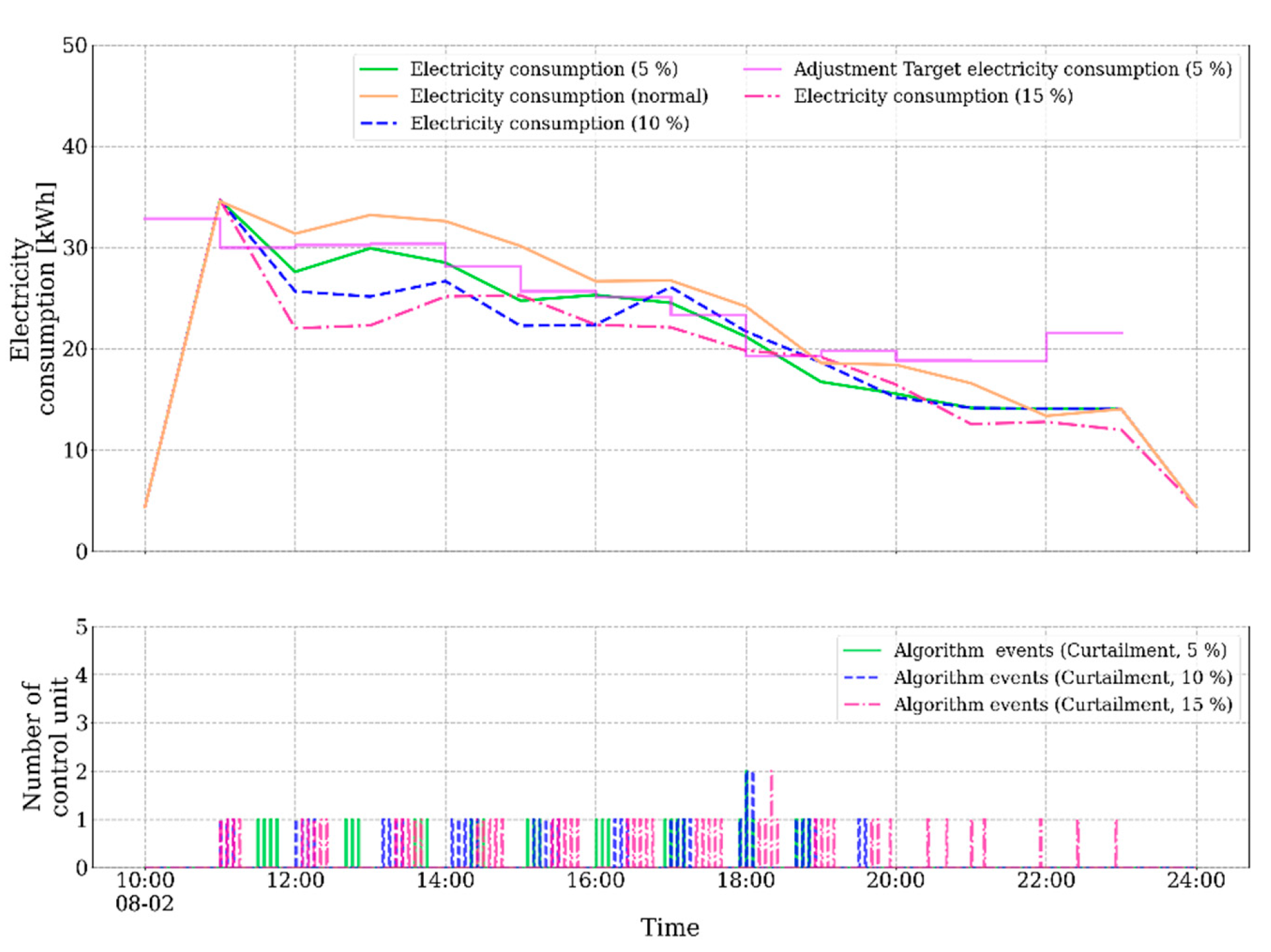
Figure 13 show the simulation result applying the building control algorithm, and the electricity consumption without the algorithm was 380.5 kWh/d. When the reduction ratio was 5%, the electricity consumption with the algorithm was 352.5 kWh/d, which was a 7.3% decrease, compared to the electricity consumption without the algorithm. When the reduction ratio was 10%, the electricity consumption was 343.4 kWh/d, which was a 9.7% decrease, and when the reduction ratio was 15%, the electricity consumption was 329.7 kWh/d, which was a 13.4% decrease. Figure 12 shows the electricity consumption with the algorithm and the predicted electricity consumption, the target electricity consumption, the algorithm event, and the operated air conditioners. In Figure 12, if the target is low, more algorithm events can proceed to match the target, but if the target if high, it means that there is a possibility that less algorithm events will proceed. Although the original occupied time of simulation progress is from 10:00 to 00:00, Figure 12 is from 10:00 to 23:00. Since the target electricity consumption at 00:00 is less than the minimum electricity consumption of 10 kWh of the simulation, it was excluded from the occupied time. Algorithm events were controlled nine times (5% reduction), 10 times (10%), and 15 times (15%). Comparing the target with the adjusted target and the electricity consumption, the adjusted target at 11:00 is applied lower than the target, because the electricity consumption at first at 10:00 is higher than the adjusted target. After 11:00, it can be seen that the adjusted target is lower than the target, because the electricity consumption is lower than the adjusted target. Under a 5% reduction ratio, since the building electricity consumption is lower than the target, the difference between the initial target and the adjustment target applied to the actual algorithm gradually increases over time, and the last algorithm time, 22:00–23:00, shows that the difference between targets is about 10 kWh. Under a 10% reduction ratio, when comparing the case with the algorithm and without the algorithm, the reason that the adjustment target rises even though it is lower than the target reduction rate is that the predicted electricity consumption is higher than that of the building without algorithm, and the target based on the predicted electricity consumption. Under a 15% reduction ratio, since the building electricity consumption is lower than the target, the difference between the initial target and the adjustment target is applied, the actual algorithm gradually increases over time, and the last algorithm time, 22:00–23:00, shows that the difference between targets gradually increases over time; but after 18:00, the building electricity consumption is a higher target, so the difference between the targets narrows, and it can be seen that the last algorithm time, 22:00–23:00, has a smaller adjustment target than the initial target. 
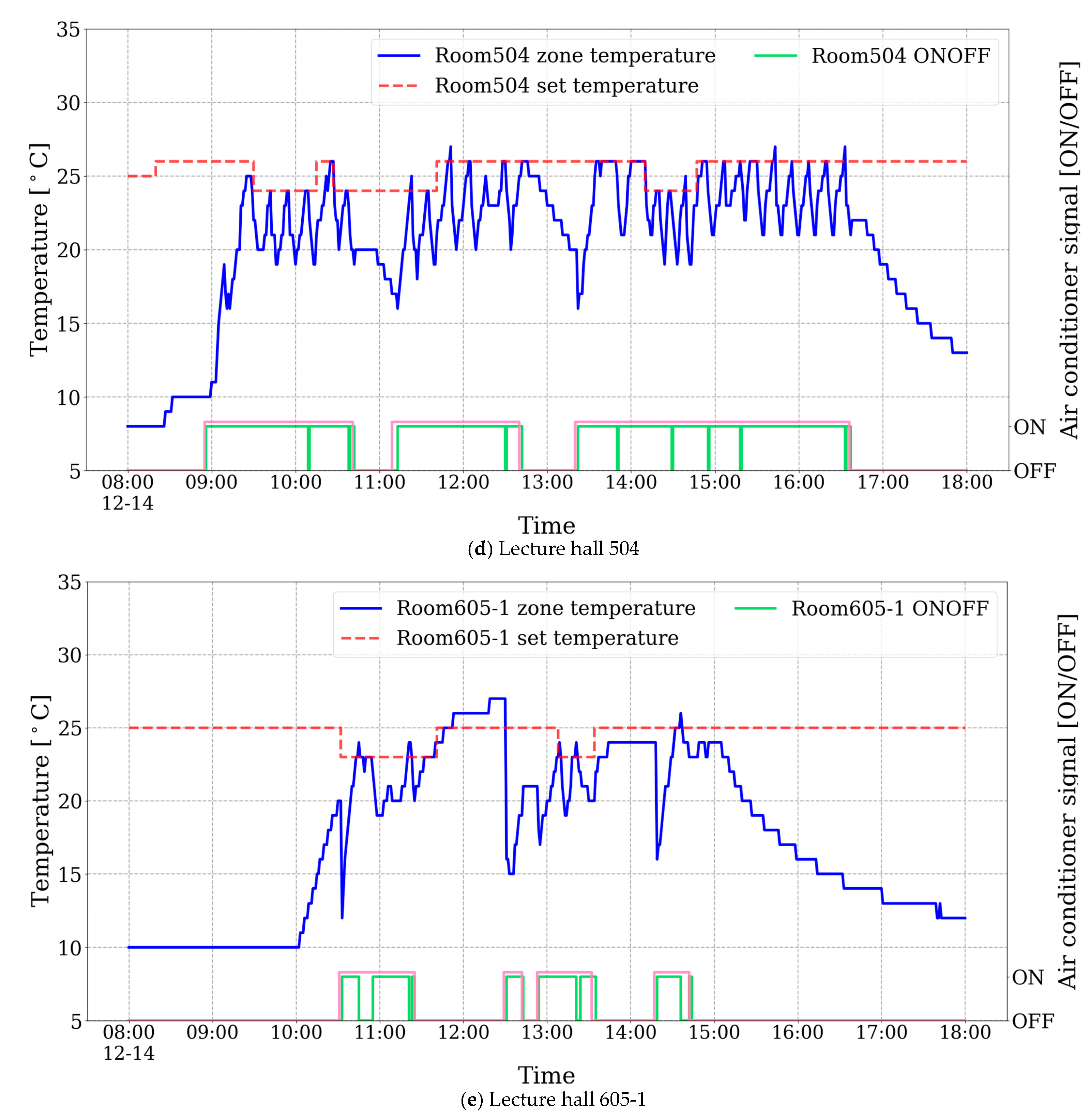
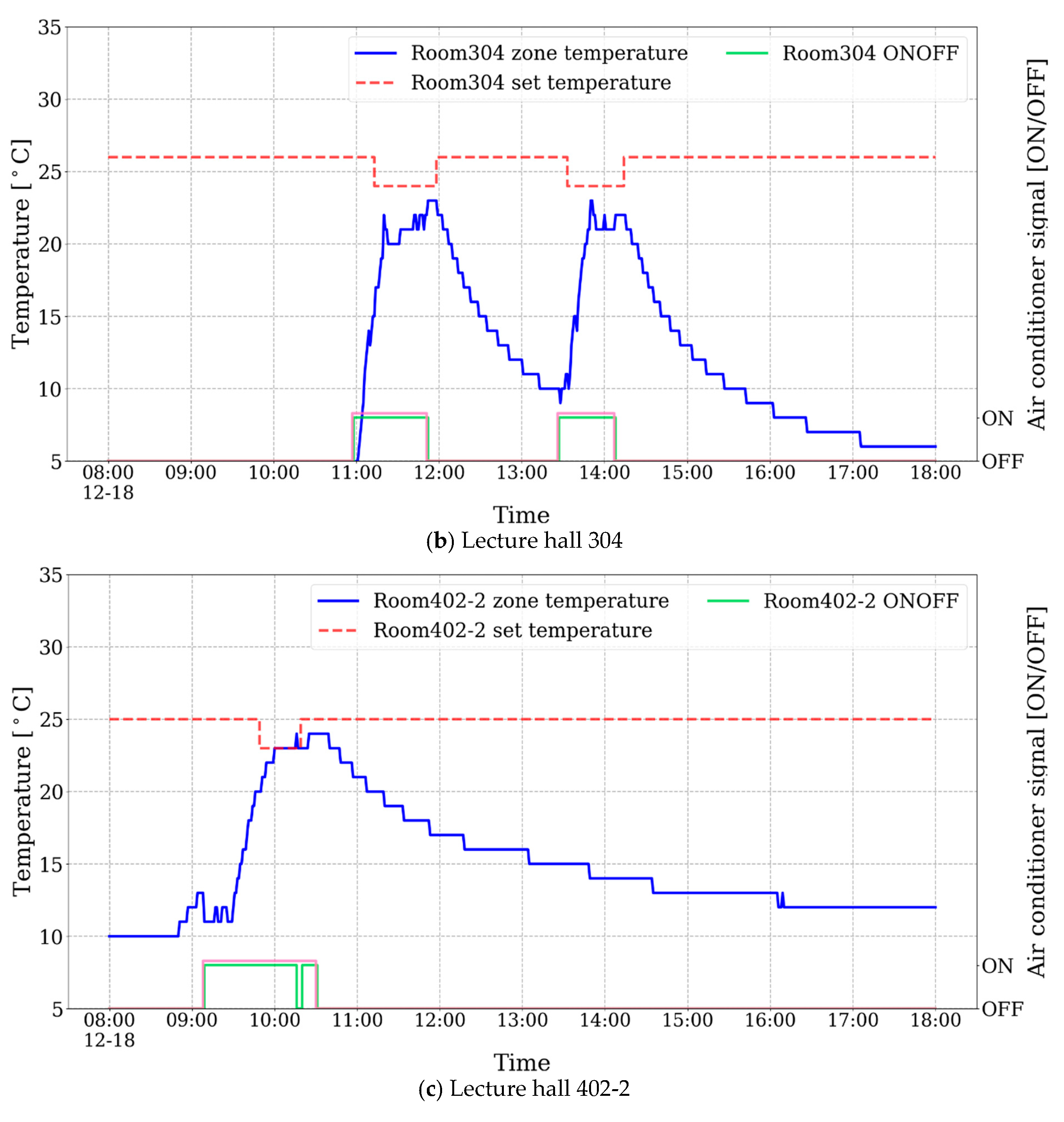
Figure 13 shows a graph of the zone temperature, set temperature, and the air conditioner status that are operated, and when an algorithm event occurs, the number of air conditioners under operational status decreases, showing that all of the controlled air conditioners during the revert time were not turned into normal operation at the same time, but that some of the controlled air conditioners were turned into normal operation, and then the remaining controlled air conditioners were returned to normal operation over time. Additionally, the maximum temperature is at 10:00, just before the air conditioner is turned on, and the algorithm was started after that. The set temperature of the air conditioner to be controlled is 26 °C and the air conditioners were often turned off and on. Figure 12 and Figure 13 show that the algorithm first starts at about 11:00, and that there are a total of four or five controlled air conditioners. Even though only one air conditioner operates, or no air conditioner operates, it can be seen that the zone temperature does not exceed 27 °C, and the control duration time is 25–35 min. Although the zone temperature exceeds the new set temperature (26 °C) during the building control algorithm, this zone temperature is not enough to cause occupant discomfort, as the air conditioner is operated when the zone temperature exceeds the new set temperature. Additionally, temperature difference between the zone and set temperature is under 1 °C. Thus, the occupant comfort is not endangered.

4.2. Field Test Result

Figure 14 shows the results of prediction of the electricity consumption using the weekly model and simulation data trained in the seq2seq LSTM structure, in order to evaluate the prediction accuracy, according to whether it is with or without Bayesian optimization. The red line shows that the input sequence length is 168 (7 d) and the output sequence length is 168 (7 d), and the patterns of the predicted value and the actual value are similar. The green line, Bayesian optimization, shows that the predicted value and the actual value have more similar patterns when compared to the model without Bayesian optimization. In addition, looking at Table 6 the prediction performance of the model with Bayesian optimization is MBE −17.1% and Cv(RMSE) 47%, which offers better prediction than the model without Bayesian optimization (MBE −46.1%, Cv(RMSE) 64.4%). Figure 15 shows the result of prediction of the electricity consumption using the daily model and simulation data trained in the seq2seq LSTM structure, in order to evaluate the prediction accuracy according to whether with or without Bayesian optimization. The red line shows that the input sequence length is 24 (1 d) and the output sequence length is 24 (1 d), and the pattern between the predicted value and the actual value is similar. The green line, Bayesian optimization, shows that when compared to the model without Bayesian optimization, the predicted value and the actual value show more similar patterns. In addition, referring to Table 6, the prediction performance of the model with Bayesian optimization is MBE 5.5% and Cv(RMSE) 39.2%, which shows better prediction than the model without Bayesian optimization (MBE −15.3%, Cv(RMSE) 48%). Table 7 shows the hyperparameters selected by Bayesian optimization.

Reduction Ratio 5% Result

Figure 16 and Figure 17 show the field test result applying the algorithm, with the total air conditioners operated in heating mode, where the predicted electricity consumption was 16,286.5 kWh/d. When the reduction ratio was 5%, the electricity consumption with the algorithm was 15,186.5 kWh/d, which, compared to the predicted electricity consumption, was a 6.8% decrease. Figure 16 shows a graph of the electricity consumption in the building, the number of operating air conditioners, and the time when the algorithm occurred, and the algorithm was controlled a total of 11 times. The blue line means the electricity consumption with the algorithm, the yellow line means the predicted electricity consumption, the red and green dotted line means the target electricity consumption, the green and pink line means the algorithm event, and the navy line means the number of operating air conditioners. In the experiments, the occupied time period is from 9:00 to 18:00, and during this period, the electricity consumption is lower than the target electricity consumption, so the adjustment target electricity consumption is higher than the initially set target (the target electricity consumption). Initially, there is not much difference between the initial target and the adjustment target electricity consumption, but the difference gradually increases with time. This is because the difference between the previous building electricity consumption and the previous target electricity consumption is distributed to the adjustment target electricity consumption in proportion to the predicted electricity consumption from the next time zone to the last time zone of the occupied time. When the target is lower than the electricity consumption, the algorithm is run more frequently, the control duration is longer, and the number of operating air conditioners is likely to decrease. Figure 17 shows a graph of the control set temperature, zone temperature, the air conditioner status of lecture hall 205-1, 3F lounge, lecture halls 403-2, 504, and 605-1 on floors 2–6, and the time when the air conditioners are turned on. While when not controlled, the set temperature used was set to 25–26 °C, the set temperature used to control the air conditioner reduced by 2 °C at the set temperature used when not controlled. The algorithm in lecture room 205-1 was controlled four times, which occurred at 9:24, 10:56, 12:47, and 17:05. The algorithm in 3F lounge 2 was controlled three times; in lecture room 403-2, two times; in lecture room 504, three times; and in lecture room 605-1, two times.
Figure 18 and Figure 19 show the field test results applying the algorithm, the total air conditioners operated heating mode, and the predicted electricity consumption was 16,874.6 kWh/d. When the reduction ratio was 10%, the electricity consumption with the algorithm was 15,267.6 kWh/d, which was a 10% decrease, compared to the predicted electricity consumption. Figure 18 shows a graph of the electricity consumption in the building, the number of operating air conditioners, and the time when the algorithm occurred, and the algorithm was controlled a total of 16 times. The blue line means the electricity consumption with the algorithm, the yellow line means the predicted electricity consumption, the red and green dotted line mean target electricity consumption, the green and pink line means the algorithm event, and the navy line means the number of operated air conditioners. In experiments, the occupied time period is from 8:00 to 18:00, and during this period, the electricity consumption is higher than the target electricity consumption, so the adjustment target electricity consumption is lower than the initially set target (target electricity consumption). Initially, there is not much difference between the initial target and the adjustment target electricity consumption, but the difference gradually increases with time. This is because the difference between the previous building electricity consumption and the previous target electricity consumption is distributed to the adjustment target electricity consumption in proportion to the predicted electricity consumption from the next time zone to the last time zone of the occupied time. When the target is lower than the electricity consumption, the algorithm is run more frequently, the control duration is longer, and the number of operated air conditioners is likely to decrease. Figure 19 shows a graph of the control set temperature, zone temperature, the air conditioner status of lecture halls 202-2, 305-2, 404, 5F lounge 1, and lecture hall 605-2 on floors 2-6, and the time when the air conditioners are turned on. While the set temperature used when not controlled was set at 25–26 °C, the set temperature used to control the air conditioner reduced by 2 °C at the set temperature used when not controlled. The algorithm in lecture room 202-2 was controlled six times, which occurred at 10:23, 11:49, 13:11, 14:11, 15:16, and 16:16. In lecture room 305-2, the algorithm was controlled five times; in lecture room 404, one time; in 5F lounge 1, six times; and in lecture room 605-2, three times.
Figure 20 and Figure 21 show the field test results applying the algorithm, the total air conditioners operated in heating mode, and that the predicted electricity consumption was 8364.1 kWh/d. When the reduction ratio was 15%, the electricity consumption with the algorithm was 7189.6 kWh/d, which compared to the predicted electricity consumption, was a 14% decrease. Figure 20 shows the electricity consumption in the building, the number of operating air conditioners, the time when the algorithm occurred, and that the algorithm was controlled a total of 10 times. The blue line means the electricity consumption with the algorithm, the yellow line means the predicted electricity, the red and green dot line means the target electricity consumption, the green and pink line means the algorithm event, and the navy line means the number of operated air conditioners. In experiments, the occupied time period is from 8:00 to 18:00, and during this period, the electricity consumption is lower than the target electricity consumption, so the adjustment target electricity consumption is higher than the initially set target (target electricity consumption). Initially, there is not much difference between the initial target and the adjustment target electricity consumption, but the difference gradually increases with time. This is because the difference between the previous building electricity consumption and the previous target electricity consumption is distributed to the adjustment target electricity consumption in proportion to the predicted electricity consumption from the next time zone to the last time zone of the occupied time. When the target is lower than the electricity consumption, the algorithm is run more frequently, the control duration is longer, and the number of operated air conditioners is likely to decrease. Figure 21 shows the control set temperature, zone temperature, the air conditioner status of lecture halls 201-1, 304, 402-2, 505-2, and 605-1 on floors 2–6, and the time when the air conditioners are turned on. While the set temperature used when not controlled was set to 25–26 °C, the set temperature used to control the air conditioner at the set temperature used when not controlled reduced by 2 °C. The algorithm in the lecture room 201-1 was controlled five times, which occurred at 9:53, 10:52, 11:37, 12:57, and 16:14. In lecture room 304, the algorithm was controlled two times; in lecture room 402-2, one time; in lecture room 505-2, four times; and in lecture room 605-1, two times.

5. Conclusions

This study proposes the building control algorithm as a technique to reduce the amount of electricity consumption in buildings, uses Seq2seq LSTM to set the target building electricity consumption in the algorithm, and uses AHP to prioritize air conditioners. The proposed algorithm is aimed at reducing the overall electricity consumption of buildings rather than the peak electricity consumption of conventional algorithms, and the target electricity consumption is selected using the predicted value of the seq2seq LSTM model. By using a predictive model, we can expect automation of target electricity consumption selection and more accurate target electricity consumption selection.
The seq2seq LSTM model was used as a method of predicting the electricity consumption of the building, and Bayesian optimization, one of the hyperparameter optimization methods, was proposed as a method of selecting an optimized hyperparameter to improve the performance of the model. It can be seen that the predicted power consumption is similar to the actual electricity consumption in all models using seq2seq LSTM, and analysis showed that when Bayesian optimization is used, the prediction accuracy of the model increases considerably.
The simulation result applying the algorithm was performed under the conditions of different reduction ratio of 5, 10, and 15%, and the actual reduction ratio during simulation was 7.3, 9.7, and 13.4%, respectively. The simulation result applying the algorithm is similar to various reduction ratios targeted by the algorithm applied to the simulation, and it was confirmed that the algorithm can effectively reduce the electricity consumption to the target building electricity consumption while maintaining occupant convenience. The field test result applying the algorithm was conducted under various target conditions, such as a reduction ratio of 5, 10, and 15%. The reduction ratios are 6.8, 10, and 14%, compared to the predicted electricity consumption for reduction ratios 5, 10, and 15%, respectively. In addition, despite turning off the air conditioner while performing algorithm, the zone temperature does not go below 20 °C, the maximum temperature of the algorithm, indicating that the algorithm reduces electricity consumption while maintaining comfort. Thus, the building control algorithm proposed in this study showed that the building electricity consumption could be matched to the target electricity consumption while maintaining occupant comfort. In addition, the field test with the building control algorithm applied to real buildings proves that the building control algorithm can be used for real buildings.

Author Contributions

Conceptualization, Y.H. and W.K.; methodology, Y.H. and W.K.; software, Y.H. and W.K.; validation, Y.H.; formal analysis, Y.H.; investigation, Y.H.; resources, Y.H.; data curation, Y.H.; writing—original draft preparation, Y.H.; writing—review and editing, W.K.; visualization, Y.H.; supervision, W.K.; project administration, W.K.; funding acquisition, W.K. All authors have read and agreed to the published version of the manuscript.

Funding

This research was supported by Basic Science Research Program through the National Research Foundation of Korea (NRF) funded by the Ministry of Education (2019R1G1A1100470) and the National Research Council of Science & Technology (NST) grant by the Korea government (MSIT) (No. CRC-15-05-ETRI).

Institutional Review Board Statement

Not applicable.

Data Availability Statement

The data presented in this study are available on request from the corresponding author.

Conflicts of Interest

The authors declare no conflict of interest.

Nomenclature

s Split function
k Covariance function
f Forget gate
i Input gate
o Output gate
g Memory cell state
c Cell state
h t Hidden state
W Weight matrix
t a n h Hyperbolic tangent function
G P Gaussian process
uUtility function
x Input set
P Electricity consumption
E Reduction ratio
u Operating status of air conditioner
T Temperature
N Period
MaxMaximum
MinMinimum
Cv(RMSE)Coefficient of variation of root-mean-square error
MBEMean bias error
Subscripts
WeekWeek
DDay
p r e d Prediction
h Hour
targetTarget
o c c Occupied time
a d j u s t Adjustment
i n v Inverse
tTime
α Weight value
c Current
SetSetting
maxSetting maximum value
minSetting minimum value
Greeks
ϕ Filter function
ψ Geometric characteristic of the partitioning function
θ Optimal value
μ Mean function
σ Sigmoid function
λ Priority of air conditioner

References

  1. Pérez-Lombard, L.; Ortiz, J.; Pout, C. A review on buildings energy consumption information. Energy Build. 2008, 40, 394–398. [Google Scholar] [CrossRef]
  2. Edenhofer, O. Climate Change 2014: Mitigation of Climate Change; Cambridge University Press: Cambridge, UK, 2015; Volume 3, p. 383. [Google Scholar]
  3. Woohyun, K.; Srinivas, K. Development and validation of an intelligent load control algorithm. Energy Build. 2019, 135, 62–73. [Google Scholar]
  4. Goetzler, W. Variable refrigerant flow systems. Ashrae J. 2007, 49, 24–31. [Google Scholar]
  5. Yabin, G.; Zehan, T.; Huanxin, C.; Guannan, L.; Jiangyu, W. Deep learning-based fault diagnosis of variable refrigerant flow air-conditioning system for building energy saving. Appl. Energy 2018, 225, 732–745. [Google Scholar]
  6. Gerrit, B.; Simon, T.; Marc, B.; Dirk, M. Real-world application of machine-learning-based fault detection trained with experimental data. Energy 2020, 198, 117323. [Google Scholar]
  7. Kaizheng, S.; Guannan, L.; Huanxin, C.; Jiangyan, L.; Jiong, L.; Wenju, H. A novel efficient SVM-based fault diagnosis method for multi-split air conditioning system’s refrigerant charge fault amount. Appl. Therm. Eng. 2016, 108, 989–998. [Google Scholar]
  8. Kang, I.; Lee, K.H.; Lee, J.H.; Moon, J.W. Artificial Neural Network–Based Control of a Variable Refrigerant Flow System in the Cooling Season. Energies 2018, 11, 1643. [Google Scholar] [CrossRef] [Green Version]
  9. Kim, D.; Cox, S.; Cho, H.; Im, P. Evaluation of energy savings potential of variable refrigerant flow (VRF) from variable air volume (VAV) in the US climate locations. Energy Rep. 2017, 3, 85–93. [Google Scholar] [CrossRef]
  10. Hong, T.; Sun, K.; Zhang, R.; Hinokuma, R.; Kasahara, S.; Yura, Y. Development and validation of a new variable refrigerant flow system model in EnergyPlus. Energy Build. 2016, 117, 399–411. [Google Scholar] [CrossRef] [Green Version]
  11. Hochreiter, S.; Schmidhuber, J. Long short-term memory. Neural Comput. 1997, 9, 1735–1780. [Google Scholar] [CrossRef] [PubMed]
  12. Kong, W.; Dong, Z.Y.; Jia, Y.; Hill, D.J.; Xu, Y.; Zhang, Y. Short-Term Residential Load Forecasting Based on LSTM Recurrent Neural Network. IEEE Trans. Smart Grid 2019, 10, 841–851. [Google Scholar] [CrossRef]
  13. Marino, D.L.; Amarasinghe, K.; Manic, M. Building Energy Load Forecasting Using Deep Neural Networks. In Proceedings of the IECON 2016-42nd Annual Conference of the IEEE Industrial Electronics, Florence, Italy, 23–26 October 2016. [Google Scholar]
  14. Shi, H.; Xu, M.; Li, R. Deep Learning for Household Load Forecasting—A Novel Pooling Deep RNN. IEEE Trans. Smart Grid 2018, 9, 5271–5280. [Google Scholar] [CrossRef]
  15. Agrawal, R.K.; Muchahary, F.; Tripathi, M.M. Long term load forecasting with hourly predictions based on long-short-term-memory network. In Proceedings of the 2018 IEEE Texas Power and Energy Conference (TPEC), College Station, TX, USA, 8–9 February 2018; pp. 1–6. [Google Scholar]
  16. Brochu, E.; Cora, V.M.; De Freitas, N. A tutorial on Bayesian optimization of expensive cost functions, with application to active user modeling and hierarchical reinforcement learning. arXiv 2010, arXiv:1012.2599. [Google Scholar]
  17. Geoffrey, K.F.T.; Kelvin, K.W.Y. Predicting electricity energy consumption: A comparison of regression analysis, decision tree and neural networks. Energy 2007, 32, 1761–1768. [Google Scholar]
  18. Cheng, F.; Fu, X.; Shengwei, W. Development of prediction models for next-day building energy consumption and peak power demand using data mining techniques. Appl. Energy 2014, 127, 1–10. [Google Scholar]
  19. Kim, D.; Braun, J.E.; Cliff, E.M.; Borggaard, J.T. Development, validation and application of a coupled reduced-order CFD model for building control applications. Build. Environ. 2015, 93, 97–111. [Google Scholar] [CrossRef] [Green Version]
Figure 1. A flow chart of the building control algorithm.
Buildings 11 00131 g001
Figure 2. Data preprocessing.
Buildings 11 00131 g002
Figure 3. Long short-term memory (LSTM) structure.
Buildings 11 00131 g003
Figure 4. Seq2seq LSTM structure.
Buildings 11 00131 g004
Figure 5. The reduced electricity consumption.
Buildings 11 00131 g005
Figure 6. The target electricity consumption.
Buildings 11 00131 g006
Figure 7. Analytical hierarchy process (AHP) structure.
Buildings 11 00131 g007
Figure 8. Simulation implementation of the building control algorithm.
Buildings 11 00131 g008
Figure 9. Field test implementation of the building control algorithm.
Buildings 11 00131 g009
Figure 10. Load forecasting result with weekly model and simulation data.
Buildings 11 00131 g010
Figure 11. Load forecasting result with daily model and simulation data.
Buildings 11 00131 g011
Figure 12. Simulation result with target, building electricity consumption and algorithm event time applying the building control algorithm.
Buildings 11 00131 g012
Figure 13. Simulation result with zone temperature and the number of operating air conditioners applying the building control algorithm. (a) Room1; (b) Room2; (c) Room3; (d) Room4.
Buildings 11 00131 g013
Figure 14. Load forecasting result with weekly model and building data.
Buildings 11 00131 g014
Figure 15. Load forecasting result with daily model and building data.
Buildings 11 00131 g015
Figure 16. Reduction ratio 5% result of the field test with the target, building electricity consumption, and algorithm events applying the building control algorithm.
Buildings 11 00131 g016
Figure 17. Reduction ratio 5% result of the field test with the zone temperature, set temperature, and air conditioners operating state applying the building control algorithm. (a) Lecture hall 205‐1; (b) 3F lounge 2; (c) Lecture hall 403‐2; (d) Lecture hall 504; (e) Lecture hall 605‐1.
Buildings 11 00131 g017aBuildings 11 00131 g017bBuildings 11 00131 g017c
Figure 18. Reduction ratio 10% result of the field test with the target, building electricity consumption, and algorithm events applying the building control algorithm.
Buildings 11 00131 g018
Figure 19. Reduction ratio 10% result of the field test with the zone temperature, set temperature, and air conditioners operating state applying the building control algorithm. (a) Lecture hall 202‐2; (b) Lecture hall 305‐2; (c) Lecture hall 404; (d) 5F lounge 1; (e) Lecture hall 605‐2.
Buildings 11 00131 g019aBuildings 11 00131 g019bBuildings 11 00131 g019c
Figure 20. Reduction ratio 15% result of the field test with the target, building electricity consumption, and algorithm events applying the building control algorithm.
Buildings 11 00131 g020
Figure 21. Reduction ratio 15% result of the field test with the zone temperature, set temperature, and air conditioners operating state applying the building control algorithm. (a) Lecture hall 201‐1; (b) Lecture hall 304; (c) Lecture hall 402‐2; (d) Lecture hall 505‐2; (e) Lecture hall 605‐1.
Buildings 11 00131 g021aBuildings 11 00131 g021bBuildings 11 00131 g021c
Table 1. Hyperparameter definition.
HyperparameterDefinitionDefault Value
Learning rateThe learning rate determines how fast it moves in the direction of the gradient.0.01
L2 regularization coefficientL2 regularization is used to control the speed of the weight decay.0.003
Number of LSTM layersThe number of LSTM layers is the number of layers between input and output layers.4
Number of LSTM cellsThe number of LSTM cells is the number of neurons (LSTM cells) per layer.128
Batch sizeThe total number of training examples present in a single batch.1000
DropoutDropout is the rate of neurons out.0.5
Total number of iterationsThe total number of iterations is the number of iterations of the training model.30,000
Table 2. Hyperparameter domain.
HyperparameterDomain
MinimumMaximum
Learning rate0.0010.05
L2 regularization coefficient0.0010.01
Number of LSTM layers15
Number of LSTM cells32128
Batch size10005000
Dropout0.00.9
Table 3. The simulation building information.
CategoryInformation
Outdoor air temperature dataTMY3 (Typical Meteorological Year 3)
Building locationPhiladelphia
Building size23.34 m width, 19.82 m depth, 3.35 m height
Normal occupied/unoccupied set points(22/30) °C
Air conditioner compressor minimum run time5 min
Table 4. Error for test data with simulation data.
ModelHyperparameter Optimization TypesMBE [%]Cv(RMSE) [%]
WeeklyManual Search−25.928.9
Bayesian optimization−3.84.9
DailyManual Search−3.714.2
Bayesian optimization−0.612.2
Table 5. Hyperparameter values with simulation data.
Hyperparameter Optimization TypesModelInput Seq. LengthOutput Seq. LengthLearning RateRegularization Coefficient # of LSTM Layers# of LSTM Cells Batch SizeDropout
ManualWeekly1681680.010.003412810000.5
Daily24240.010.003412810000.5
BayesianWeekly1681680.0250.00621198910.435
Daily24240.010.00121274750.1
Table 6. Error for test data with simulation data.
ModelHyperparameter Optimization TypesMBE [%]Cv(RMSE) [%]
WeeklyManual Search−46.164.4
Bayesian optimization−17.147
DailyManual Search−15.348
Bayesian optimization5.539.2
Table 7. Hyperparameter values with simulation data.
Hyperparameter Optimization TypesModelInput Seq. LengthOutput Seq. LengthLearning RateRegularization Coefficient # of LSTM Layers# of LSTM CellsBatch SizeDropout
ManualWeekly1681680.010.003412810000.5
Daily24240.010.003412810000.5
BayesianWeekly1681680.0240.00823613260.01
Daily24240.0130.002311519080.8
Publisher’s Note: MDPI stays neutral with regard to jurisdictional claims in published maps and institutional affiliations.

