Effects of the Earthquake Nonstationary Characteristics on the Structural Dynamic Response: Base on the BP Neural Networks Modified by the Genetic Algorithm

Abstract

The intensity non-stationarity is one of the basic characteristics of ground motions, the influences of which on the dynamic responses of structures is a pressing issue in the field of earthquake engineering. The BP neural network modified by the genetic algorithm was adopted in this research to investigate the influence of intensity nonstationary inputs on the structural dynamic responses from a new perspective. Firstly, many training data were generated from the prediction formula of dynamic response. The BP neural network was then pre-trained by sparsely selected data to optimize the initial weights and biases. Finally, the BP neural network was trained by all data, and the mean square error of predicted responses compared with the target response were less than 10⁻⁵. The calculation formula of sensitivity was also derived here to quantify the influence of the input change on the output. The presented method combines the advantages of neural networks in nonlinear multi-variable fitting and provides a new perspective for the study of earthquake nonstationary characteristics and their influence on the structural dynamic responses.

1. Instruction

The intensity non-stationarity of ground motions refers to the characteristic that the energy of ground motions changes over time, the performance of which is that the amplitude of the acceleration time history gradually increases and finally attenuates to zero. Artificial ground motions time history needs to be generated since there are usually only a few of the ground motions required for nonlinear time-history analysis. Research on the intensity non-stationarity of ground motions is focused, first, on generating many ground motions meeting the time-history analysis requirements by using the rule of intensity non-stationarity and, more importantly, studying the effect of the earthquake non-stationarity characteristics on the structural dynamic responses.

In the conventional research [1,2,3,4,5], the intensity non-stationarity of ground motions is mainly described from the perspective of the intensity envelope functions of ground motions. The shape of these intensity envelope functions is controlled by a number of shape parameters, and the artificial ground motion with intensity non-stationarity can be obtained by modulating a stationary ground motion using the envelope function. The value of the shape parameters is also a focus of the research on the intensity non-stationarity, and the previous methods based on engineering experience no longer meet the needs of engineering application. Huo et al. [6] fit the attenuation relationship of envelope parameters with magnitude, epicentral distance and site conditions by statistical method for three-step intensity envelope functions. Qu et al. [7] fit the change rule of parameters of the three-step intensity envelope function using the three seismic records of SMART-1 array and analyzed the effect of the coordinates and soil thickness of the measuring points on the parameters. Du et al. [8] proposed an intensity envelope function with log-normal distribution, fit the attenuation relationship of envelope parameters with magnitude and epicentral distance under different site conditions by statistical method, and gave the recommended values under different conditions.

The effect of the intensity non-stationarity of ground motions on the structural dynamic responses is not insignificant. Liu et al. [9] analyzed the effect of the envelope parameters of three-step intensity envelope function on the structural responses and obtained the approximate quantitative relationship between the parameters of the intensity non-stationarity of ground motions and the structural responses by fitting, which suggested that the stationary state duration of ground motions had a significant effect on the structural seismic responses. Jiang et al. [10] deduced the analytical expression of structural dynamic responses activated by the intensity non-stationarity based on the damped-sine function, which suggested that the frequency ratio and non-stationarity had a greater effect on the maximum value of structural dynamic responses than the damping ratio.

There are two main kinds of methods for researching earthquake non-stationarity characteristics and their influence on structural dynamic responses: analytical methods and numerical methods. With the analytical methods, the effect rule obtained is accurate and intuitive, but we can only obtain the analytical expression of displacement response time history, which is extremely complex. On the one hand, it is difficult to derive the expressions for velocity and acceleration. On the other hand, numerical methods are still needed to obtain the maximum value of responses. However, in general numerical methods, the values at multiple discrete points are calculated first, and then a smooth curve is used to fit the change rule. This method is feasible in the case of low dimension where there are few parameters but can hardly be implemented when there are many parameters. Therefore, neural networks are proposed in this paper to study the effect of the intensity non-stationarity of ground motions on the structural responses. Neural networks have a strong high-dimensional nonlinear fitting capacity. In this paper, the formula for the sensitivity of input parameters is deducted based on this, and, compared with the results of the analytical formula, this method could accurately analyze the change rule and influence of the maximum value of the structural responses with the parameters of the intensity non-stationarity.

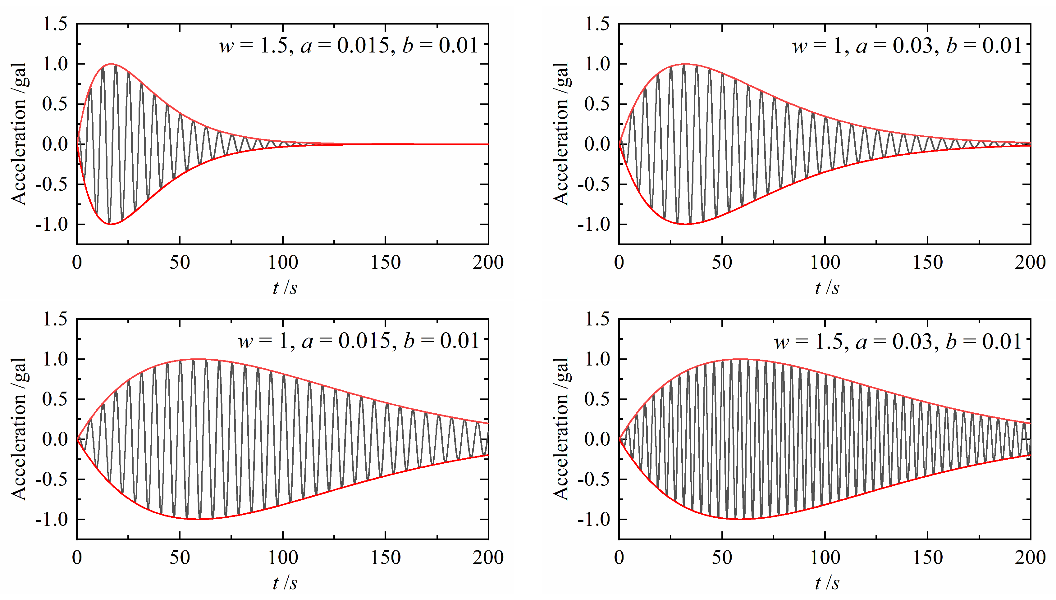
2. The Intensity Non-Stationarity Model Enveloped by the Damped-Sine Function and the Analytical Solution of Its Dynamic Responses

The damped-sine function typed intensity envelope function was proposed by Shinozuka et al. [1], as follows:

$$\begin{array}{l}f\left(t\right)=I_0{e}^{-\alpha t}\sin \left(\beta t\right)\\ I_0=\frac{e^{\alpha t_0}}{\sin \beta t_0}\\ t_0=\frac{1}{\beta }arctg\frac{\beta }{\alpha }\end{array}$$

(1)

where f(t) is the damped-sine function typed intensity envelope function; I₀ is the normalization constant, which uniformly adjusts the peak of the envelope function to 1; α is the parameter of the attenuation term, which mainly affects the peak position and attenuation rate of the envelope function; β is the excitation shape parameter as well as the frequency of the sine function, which mainly controls the descent rate of the envelope function in the descent segment, with little influence on the peak position; and t₀ is the time of the peak of the envelope function. The analytical expression (Equation (2)) of the intensity non-stationarity signal based on the damped-sine function can be obtained by modulating a cosine wave with f(t), where ω is the circular frequency of the analytical signal. The typical expression of F(t) is shown in Figure 1.

$$F\left(t\right)=I_0{e}^{-\alpha t}\sin \left(\beta t\right)\cos \left(\omega t\right)$$

(2)

The equation of motion shown in Equation (3) can be obtained when the modulated non-stationarity analytical signal F(t) is input into a single-degree-of-freedom.

$$\frac{d^{2}u}{d{t}^2}+2\zeta {\omega }_n\frac{du}{dt}+{\omega }_n^{2}u=-I_0{e}^{-\alpha t}\sin \left(\beta t\right)\cos \left(\omega t\right)$$

(3)

where u is the displacement responses of the structure, the first- and second-order derivatives of which are velocity response and acceleration response; ζ is the damping ratio; and ω_n is the structural natural vibration circular frequency. JIANG et al. [10] obtained the analytical expression (Equation (4)) of the displacement response u(t) by the Laplace transformation on both sides of Equation (3).

$$\begin{array}{cc}\hfill u\left(t\right)& =-\frac{I_0}{2}\{\left(\beta +\omega \right)[e^{\alpha t}\frac{2A\sin \left(\beta +\omega \right)t-2B\cos \left(\beta +\omega \right)t}{A^2+B^2}+\hfill \\ & e^{-\zeta {\omega }_{n}t}\frac{2C\sin \left({\omega }_{n}t\sqrt{1-{\zeta }^2}\right)-2D\cos \left({\omega }_{n}t\sqrt{1-{\zeta }^2}\right)}{C^2+D^2}]\}-\hfill \\ & \frac{I_0}{2}\{\left(\beta +\omega \right)[e^{\alpha t}\frac{2A_1\sin \left(\beta +\omega \right)t-2B_1\cos \left(\beta +\omega \right)t}{A_1^2+B_1^2}+\hfill \\ & e^{-\zeta {\omega }_{n}t}\frac{2C_1\sin \left({\omega }_{n}t\sqrt{1-{\zeta }^2}\right)-2D_1\cos \left({\omega }_{n}t\sqrt{1-{\zeta }^2}\right)}{C_1^2+D_1^2}]\}\hfill \end{array}$$

(4)

where

$$\begin{array}{l}A=2\left(\beta +\omega \right)\left[{\left(\zeta {\omega }_n-a\right)}^2-{\left(\beta +\omega \right)}^2+\left({\omega }_n^2-{\omega }_n^2{\zeta }^2\right)\right]\\ B=4{\left(\beta +\omega \right)}^2\left(\zeta {\omega }_n^2-a\right)\\ C=2{\omega }_n\sqrt{1-{\zeta }^2}\left[{\left(a-\zeta {\omega }_n\right)}^2-{\omega }_n^2\left(1-{\zeta }^2\right)+{\left(\beta +\omega \right)}^2\right]\\ D=4{\omega }_n^2\left(1-{\zeta }^2\right)\left(a-\zeta {\omega }_n\right)\\ A_1=2\left(\beta -\omega \right)\left[{\left(\zeta {\omega }_n-a\right)}^2-{\left(\beta -\omega \right)}^2+\left({\omega }_n^2-{\omega }_n^2{\zeta }^2\right)\right]\\ B_1=4{\left(\beta -\omega \right)}^2\left(\zeta {\omega }_n^2-a\right)\\ C_1=2{\omega }_n\sqrt{1-{\zeta }^2}\left[{\left(a-\zeta {\omega }_n\right)}^2-{\omega }_n^2\left(1-{\zeta }^2\right)+{\left(\beta -\omega \right)}^2\right]\\ D_1=4{\omega }_n^2\left(1-{\zeta }^2\right)\left(a-\zeta {\omega }_n\right)\end{array}$$

The above analytical analysis shows that the earthquake non-stationarity characteristics has an effect on the structural dynamic responses, but the expression above is too complex.

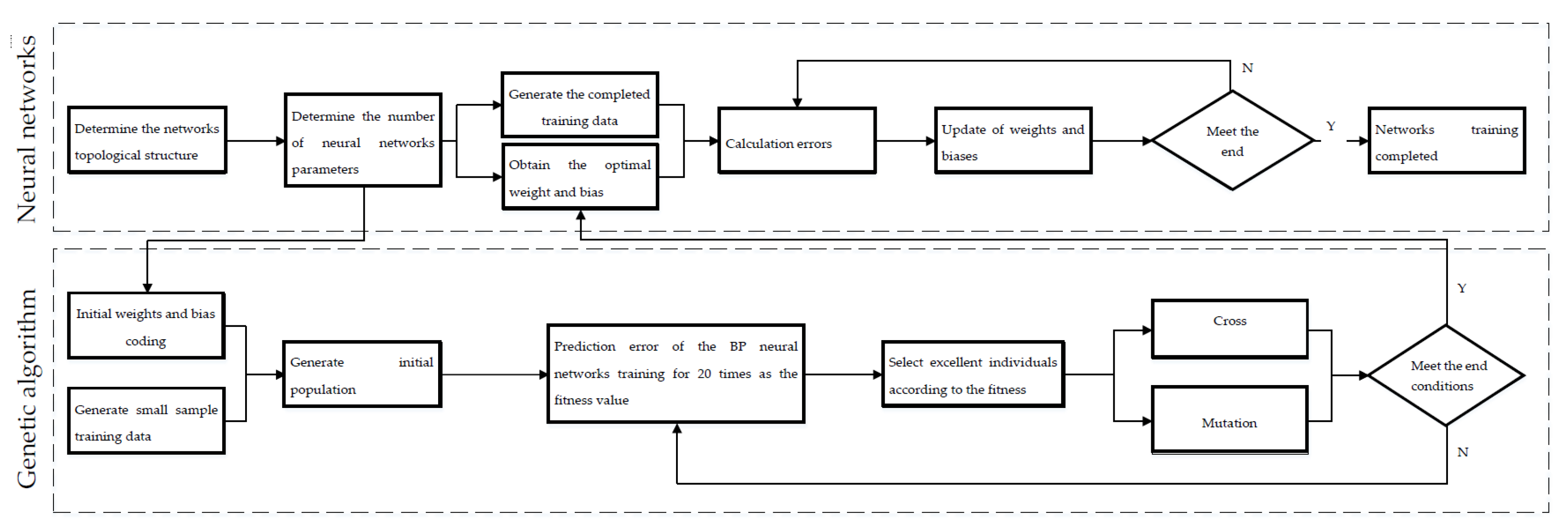
3. Response Prediction Based on the GA-BP Neural Networks

In BP neural networks, many input and output data pairs are used to optimize the initial weights and biases to minimize the error of the predicted output compared with the target output of BP neural works. The training algorithm of neural networks is an optimization algorithm based on local gradient, so the final training result is related to both initial weights and initial biases, and improper initial network parameters may cause the local optimal solution of the algorithm.

The biological evolution principle of “survival of the fittest” is introduced into the parameter optimization algorithm by genetic algorithm, and the basic operators of genetic algorithm such as selection, cross, and mutation are used to screen the individuals in the population, with the superior ones retained to produce the next generation. The process is repeated until the condition of convergence is met. Different from BP neural networks, the genetic algorithm is a global searching algorithm, which makes up for the deficiency of the poor global searching capacity of BP neural networks, and the combined model of neural networks and the genetic algorithm is called GA-BP neural networks [11,12]. In this paper, the GA-BP neural network is adopted. First, the genetic algorithm is used to optimize the initial network parameters on a small sample, and then the BP neural network is assigned to the optimized weights and biases and trained on the whole dataset to obtain the final solution. The basic algorithm flowchart of GA-BP is shown in Figure 2.

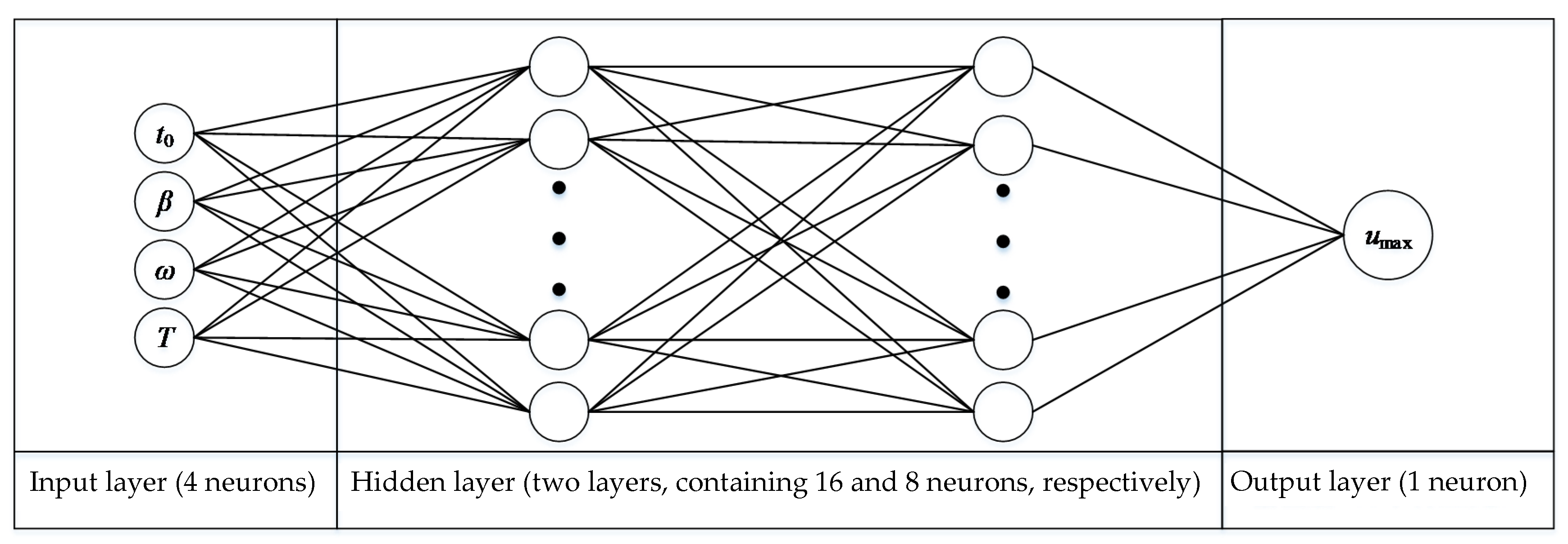
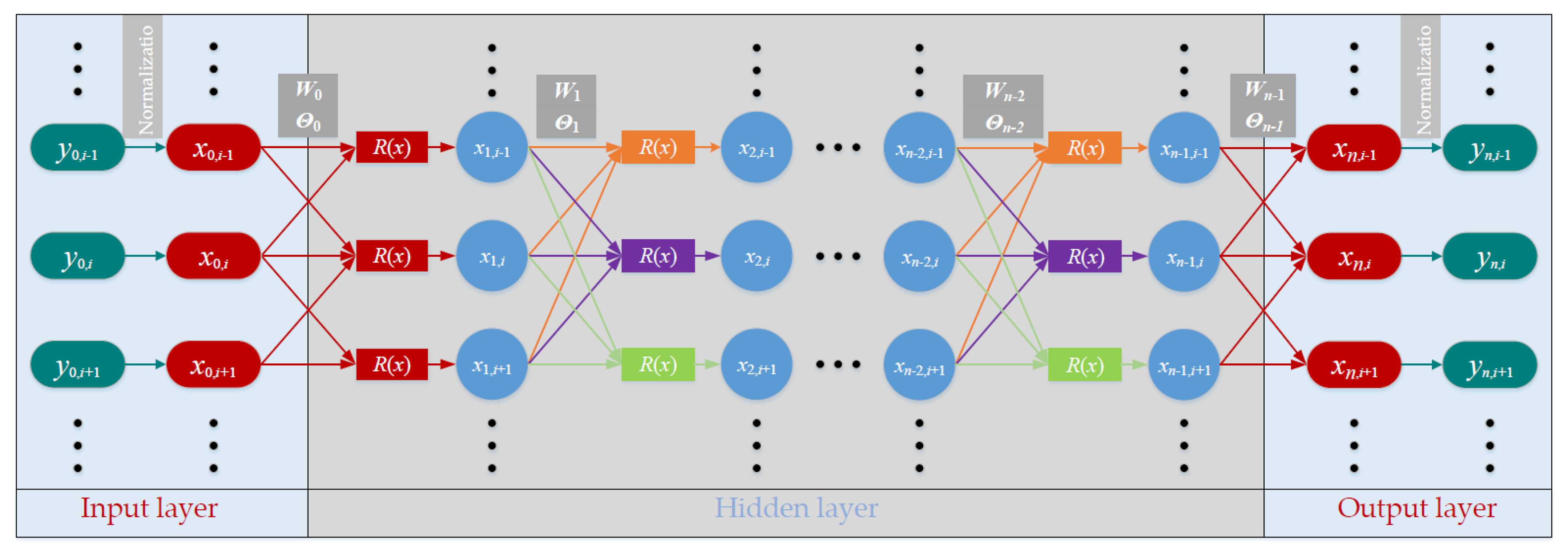
3.1. Hyperparameters of the BP Neural Networks

Different from the parameters obtained by gradient descent training, the hyperparameters of the neural networks are set before learning, including the number of layers of neural networks, the number of neurons at each layer, the selection of cost function, the selection of excitation function, the methods of weight initialization, and so on.

The intensity non-stationarity model based on the damped-sine function has four independent variable input parameters and one output parameter. The input parameters are the time of peak (t₀), parameter of excitation shape (β), excitation frequency (ω), and structural natural vibration period (T), while the output is the absolute value of the maximum displacement response (u_max) of the structure. Therefore, four neurons are needed at the input layer and one neuron is needed at the output layer of the BP neural network. In this paper, two hidden layers are set in the BP neural network, which contain 16 and 8 neurons, respectively. The structure of the artificial neural network is shown in Figure 3. The activation function of each hidden layer is a hyperbolic tangent function, and the output layer is a linear transfer function. The hyperparameters of the artificial neural network are shown in

Table 1. Hyperparameters of the artificial neural network.

Layer	Activation Function	Number of Weights	Number of Biases	Total Number of Parameters
Input layer → Hidden layer 1	Hyperbolic tangent	4 × 16 = 64	16	80
Hidden layer 1 → Hidden layer 2	Hyperbolic tangent	16 × 8 = 128	8	136
Hidden layer 2 → Output layer	Linear transfer	8 × 1 = 8	1	9
Total for each layer	-	200	25	225

.

3.2. Training Dataset

The dynamic response prediction algorithm based on the BP neural network in this paper is a supervised learning algorithm, and the training data are composed of input and output data pairs. First, values of the four input parameters are taken uniformly within a certain range to obtain a set of input data. Then, each of the input parameters is substituted into Equation (4) to obtain the displacement response time history. Finally, the maximum absolute value of the displacement response time history is taken to obtain the output of each input parameter.

Given that the fitness function of each individual in a population needs to be evaluated by the genetic algorithm, the use of all training data will cause low efficiency of the algorithm. Therefore, the training data are divided into two parts, of which the sparsely selected sample data in the first part are used to optimize the initial weights and biases of the genetic algorithm, and all data in the second part are used to train the final BP neural network. The detailed methods for taking the small sample training data and the whole training data are shown in

Table 2. Samples used for training and validation.

Data Type		Small Sample Data	Whole Data
t0	Lower limit	20	20
	Upper limit	40	40
	Interval	2	1
β	Lower limit	0.01	0.01
	Upper limit	0.05	0.05
	Interval	0.01	0.01
ω	Lower limit	1	0.1
	Upper limit	10	10
	Interval	1	0.1
T	Lower limit	0.5	0.5
	Upper limit	4	4
	Interval	0.5	0.1
Total sample		4400	378,000

.

The training dataset of the BP neural network includes training set, validation set, and test set. The training set is used to train the BP neural networks. The validation set is used to evaluate the performance of the BP neural networks, including determining whether there is underfitting or overfitting. The test set is used to evaluate the generalization ability of the final BP neural networks and does not participate in the training of the BP neural networks. In this paper, after the dataset is out of order, 70% of the total sample is randomly selected as the training set, 15% as the validation set, and 15% as the test set.

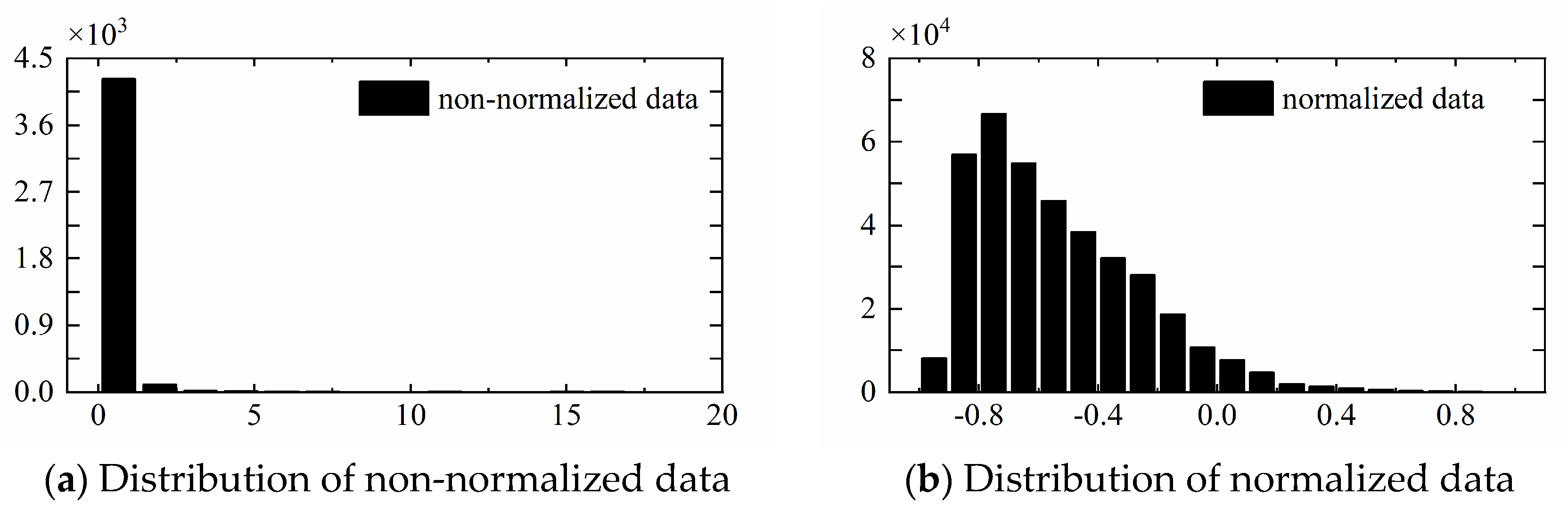
3.3. Data Initialization

In general, the distribution form of training dataset will affect the calculation efficiency of gradient descent algorithm, and data preprocessing can improve the solving speed and accuracy. The common normalization methods include linear normalization, mean standardization, and nonlinear normalization (taking the logarithm, exponent, etc.). The distribution characteristics of the training dataset in this paper show that data are too concentrated in an interval of smaller magnitude and thus the combination of linear normalization and nonlinear normalization, that is, taking the logarithm of the dataset and then normalizing the linearity, is selected, and the calculation formulas for the normalization of input and output data are shown in Equations (5) and (6), respectively.

$$y=N_1\left(x\right)=\frac{\left(m-n\right)\left(x-x_{\min }\right)}{x_{\max }-x_{\min }}+n$$

(5)

$$y=N_2\left(x\right)=\frac{\left(m-n\right)\left(\log \left(x\right)-\log \left(x_{\min }\right)\right)}{\log \left(x_{\max }\right)-\log \left(x_{\min }\right)}+n$$

(6)

where x and y are the non-normalized and normalized data, respectively; m and n are the maximum and minimum values of linear normalization, respectively; and x_max and x_min are the maximum and minimum values of the dataset, respectively. In Equation (5), the dataset is linearly compressed into the interval of [n, m]. In Equation (6), the dataset is linearly compressed into the interval of [n, m] after taking the algorithm. In this paper, n and m are set to −1 and 1, respectively, and the u_max histograms of network output before and after the normalization are shown in Figure 4. It can be seen that many non-normalized data are concentrated in the interval of [0, 5000], while the normalized data are close to being normally distributed. Training data in normal distribution can improve the accuracy and efficiency of gradient descent algorithm.

3.4. Optimization of Initial Network Parameters Based on the Genetic Algorithm

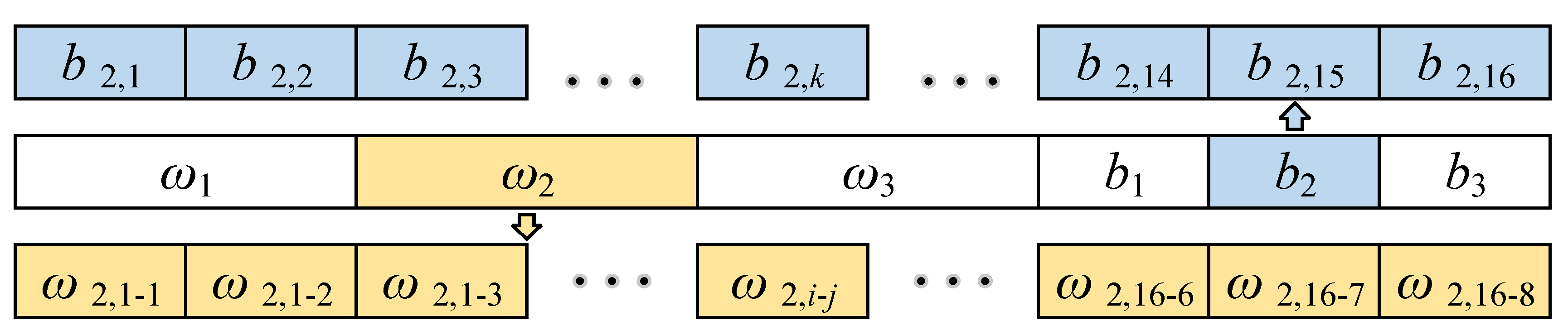
3.4.1. Coding

In the genetic algorithm, chromosome coding is needed first, with such methods as binary coding and real-number coding. For binary coding, the network parameters need to be converted into binary numbers, and the large number of parameters of the neural networks will lead to long genes. In addition, Hancock [13] pointed out in his research that binary coding will also lead to permutation problem. For real-number coding [14,15,16], the network parameters are directly coded into a string of real numbers in sequence, which requires no conversion of number systems and will not cause too long chromosome. In this paper, the real-number coding shown in Figure 5 is adopted. We can see that the chromosome consists of three sets of weight vectors and three sets of bias vectors, where ω₁, ω₂, and ω₃ are the weight vector from the input layer to the first hidden layer, the weight vector from the first hidden layer to the second hidden layer, and the weight vector from the second hidden layer to the output layer, respectively. ω_2,i-j is the weight from the ith neuron at the first hidden layer to the jth neuron at the second hidden layer. b₁, b₂, and b₃ are the bias vector from the input layer to the first hidden layer, the bias vector from the first hidden layer to the second hidden layer, and the bias vector from the second hidden layer to the output layer, respectively. b_2,k is the kth bias from the first hidden layer to the second hidden layer.

3.4.2. Fitness Function

Fitness function is used to evaluate the superiority and inferiority of each individual in a population. In this paper, the BP neural network is assigned to the chromosomes of each individual, trained 20 times, and the sum of the absolute values of prediction errors was taken as the fitness value of the individual. The calculation formula is shown in Equation (7).

$$F={\displaystyle \sum _{i=1}^n\left|y_i-o_i\right|}$$

(7)

where n is the total number of training data, which is set to 4400 in this paper; y_i is the target output of the ith set of data; and o_i is the predicted output of the ith set of data.

3.4.3. Basic Operators of Genetic Algorithm

(1)

Section operator

Roulette algorithm is selected for the selection operator in this paper, and the selection probability (p_i) is assigned to each individual based on Equation (8). In the equation, F_i is the fitness value of an individual. Since the fitness is defined as the sum of the absolute values of prediction errors, individuals with lower fitness values should be more likely to be selected.

$$p_i=\frac{{\displaystyle \prod _{j=1}^N{F}_j}}{F_i{\displaystyle \sum _{j=1}^N{F}_j}}$$

(8)

(2)

Cross operator

In this paper, the real-number cross method is adopted, and the cross probability is set to 0.3. Two paternal chromosomes are randomly selected first, and then one cross position is randomly selected. The value of the daughter chromosomes at the cross position is the randomly weighted sum of the value of two paternal chromosomes at the cross position, as shown in Equation (9).

$$\{\begin{array}{l}{A}_j^{\prime }=A_j\left(1-b\right)+B_{j}b\\ B_j^{\prime }=B_j\left(1-b\right)+A_{j}b\end{array}$$

(9)

where A′ and B′ represent the cross-generated daughter chromosomes; A_j and B_j represent the jth cross position of chromosomes A and B, respectively; j is a random integer, the maximum value of which is the length of the chromosome; and b is a randomly generated combination weight coefficient, the value range of which is from 0 to 1.

(3)

Mutation operator

In this paper, the mutation probability is set to 0.3, and it is based on Equation (10).

$$A_j^{\prime }=\{\begin{array}{l}{A}_j+r_2\left(A_j-A_{j,max}\right)\Phi \left(1-\frac{g}{G_{\max }}\right), \mathrm{when} r_1\ge 0.5\\ A_j+r_2\left(A_{j,min}-A_j\right)\Phi \left(1-\frac{g}{G_{\max }}\right), \mathrm{when} r_1<0.5\end{array}$$

(10)

where A_j is the jth gene position of a certain chromosome in a population; $A_j^{\prime }$ is the gene value on the jth gene position after mutation; A_j,max is the upper limit of the gene value on the jth gene position; A_j,min is the lower limit of the gene value on the jth gene position; r₁ and r₂ are two random numbers in [0, 1]; g is the current generation; and G_max is the maximum generation. Φ is a mutation parameter related to the generation; the greater the generation is, the smaller the value of the mutation parameter will be, i.e., the mutation probability will decrease with the increase of the generation.

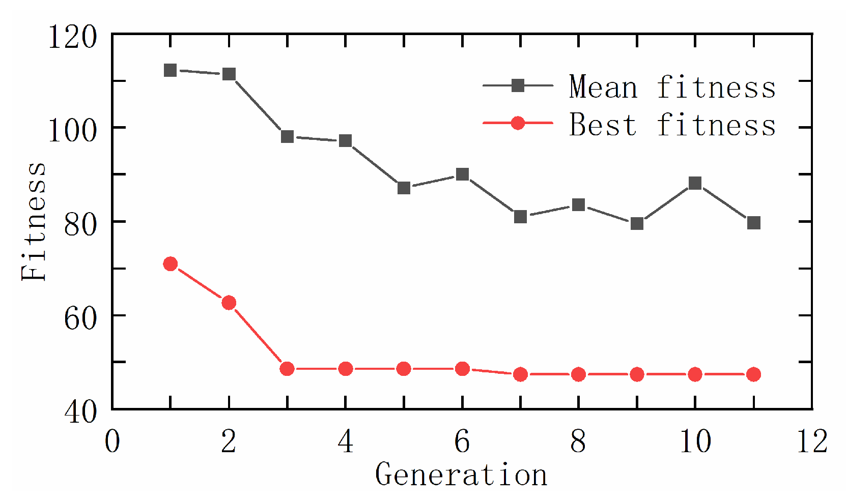
3.5. Genetic Algorithm Optimization Results

An initial population containing 20 individuals is randomly generated, and the evolution of the mean fitness values and best fitness values of a population can be obtained after 10 generations, as shown in Figure 6. It can be seen that the fitness of the population decreases constantly with the increase of the generation and finally tends to be stable.

4. Validation of the Artificial Neural Networks

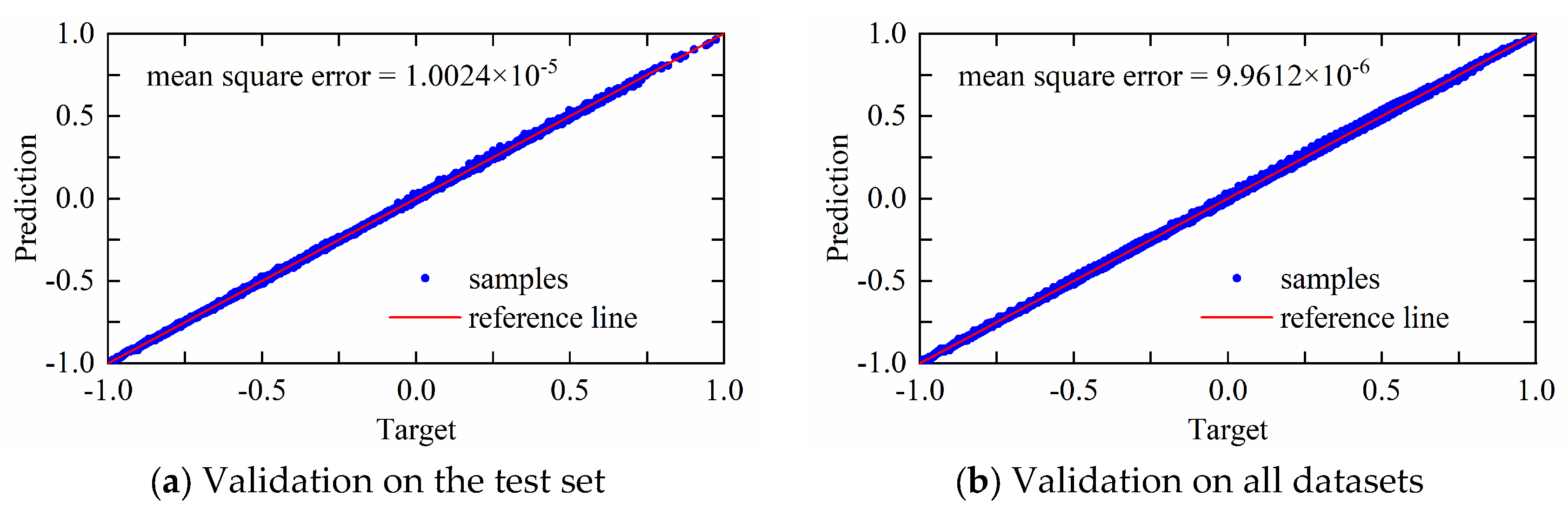
4.1. Validation on the Dataset

The predicted output of each input can be obtained after inputting the input data into the trained artificial neural networks. The validation diagram of neural networks shown in Figure 7 can be obtained with the target value as the x-coordinate and the predicted value as the y-coordinate. The closer the discrete points in the figure are to the line with a slope of 1, the higher the prediction accuracy will be.

Figure 7a shows the validation results of data on the test set, from which we can find that the discrete points are basically distributed near the line, with the mean square error of only 1.0024 × 10⁻⁵. The test set does not participate in the network training, indicating that the artificial neural network has good generalization ability. Figure 7b shows the validation results of data on all datasets, from which we can find that the mean square error is less than 10⁻⁵, indicating that the artificial neural network has higher prediction accuracy and can meet the need for subsequent analysis.

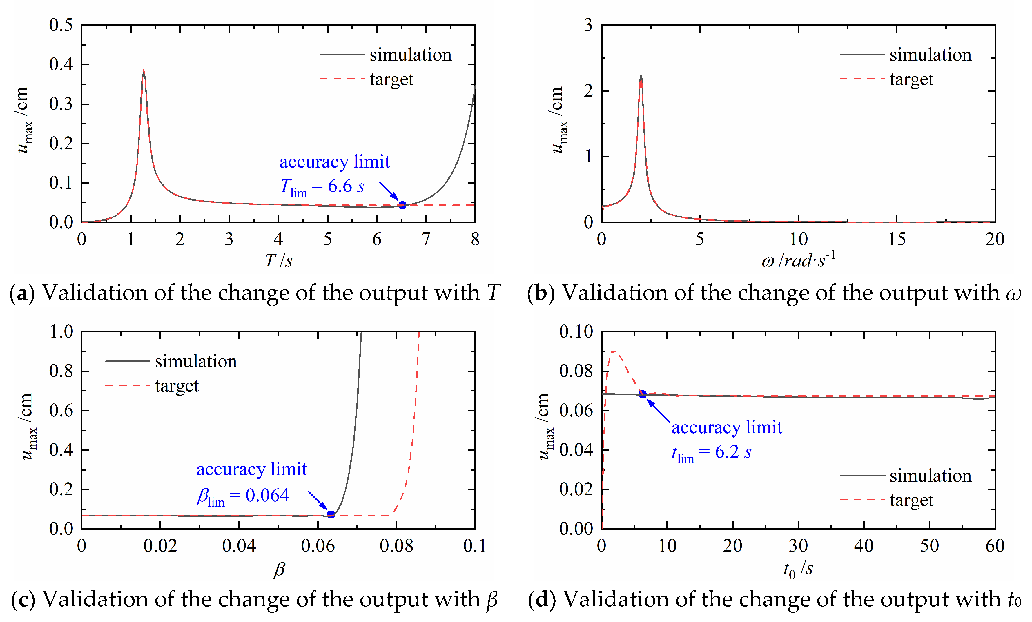
4.2. Validation of the Change Rule of Single Parameter

Test set does not participate in the artificial neural networks training, and validation of the accuracy of the artificial neural networks on the test set can effectively validate the generalization ability of the artificial neural network to some extent. However, the data values on the test set are still included in the maximum and minimum values of the training data. To further validate the generalization ability of the artificial neural networks outside the datasets, the difference between the predicted value and the theoretical value of the artificial neural network is compared by constantly changing the value of a single input parameter in this section, as shown in Figure 8.

Figure 8a shows the change of the theoretical output and predicted output with the structural period T, which can also be considered as the displacement response spectrum. When the range of T is extended from the 0.5–4 s of the original data to 0–8 s, the artificial neural networks in this paper can still accurately predict the output values before 6.6 s. Figure 8b shows the change of the theoretical output and predicted output with the excitation frequency ω. When the range of ω is extended from the 0.1–10 of the original data to 0–20, the artificial neural networks can still accurately predict the output values in the entire extended data segment. Figure 8c shows the change of the theoretical output and predicted output with the excitation shape parameter β. When the range of β is extended from the 0.01–0.05 of the original data to 0–0.1, the artificial neural networks can still accurately predict the output values in the segment before 0.064. Figure 8d shows the change of the theoretical output and predicted output with the time of peak t₀. When the range of t₀ is extended from the 20–40 s of the original data to 0–60 s, the artificial neural networks can still accurately predict the output values in the segment after 6.2 s.

5. Analysis of Influence of the Intensity Non-Stationarity of Ground Motions

5.1. Sensitivity Analysis of Neutrons at the Adjacent Layers

The complete structure of artificial neural networks is shown in Figure 9, including the input layer, hidden layer, and output layer. x_i,j represents the jth neuron at the ith layer; ReLU is the activation function; and W_i and θ_i are, respectively, the weight matrix and bias vector from the ith layer to the (i + 1)th layer.

Sensitivity [17,18] is defined as the influence of the input change on the output, which can be obtained by taking the derivative of the output with respect to the input. The mth neuron x_k,m at the kth layer and the nth neuron x_k+1,n at the (k + 1)th layer were investigated. When a neuron at the previous layer produces little disturbance, the change of the neuron at the later layer S_{(k,m),(k+1,n)} can be obtained by taking the derivative of the output x_k+1,n with respect to the input x_k,m, as shown in Equation (11).

$$S_{\left(k,m\right),\left(k+1,n\right)}=\frac{\partial x_{k+1,n}}{\partial x_{k,m}}$$

(11)

The relationship between x_k,m and x_k+1,n is shown in Equation (12), where W_k,i,n is the weight coefficient from the ith neuron at the kth layer to the nth neuron at the (k + 1)th layer; θ_k,n is the bias coefficient from the neurons at the kth layer to the nth neuron at the (k + 1)th layer; and R(x) is an activation function.

$$x_{k+1,n}=R\left[{\displaystyle \sum _i{x}_{k,i}{W}_{k,i,n}+{\theta }_{k,n}}\right]$$

(12)

After substituting Equation (12) into Equation (11), we can obtain the sensitivity expression:

$$\frac{\partial x_{k+1,n}}{\partial x_{k,m}}=\frac{\partial }{\partial x_{k,m}}R\left({\displaystyle \sum _i{x}_{k,i}{W}_{k,i,n}+{\theta }_{k,n}}\right)=R^{\prime }\left({\displaystyle \sum _i{x}_{k,i}{W}_{k,i,n}+{\theta }_{k,n}}\right)W_{k,m,n}$$

(13)

When the activation function is a linear transfer function, R(x) = x and R′(x) = 1; therefore, Equation (13) can be further simplified to Equation (14).

$$S_{\left(k,m\right),\left(k+1,n\right)}=\frac{\partial x_{k+1,n}}{\partial x_{k,m}}=W_{k,m,n}$$

(14)

When the activation function is a hyperbolic tangent function, R(x) = (e^x − e^−x)/(e^x + e^−x) and R′(x) = 1 − R²(x); therefore, Equation (13) can be further simplified to Equation (15).

$$S_{\left(k,m\right),\left(k+1,n\right)}=\left[1-R^2\left({\displaystyle \sum _i{x}_{k,i}{W}_{k,i,n}+{\theta }_{k,n}}\right)\right]W_{k,m,n}=\left(1-x_{k+1,n}^2\right)W_{k,m,n}$$

(15)

5.2. Sensitivity Analysis of Neutrons at any Layer

The mth neuron x_k,m at the kth layer and the nth neuron x_v,n at the vth layer were investigated, and their sensitivity can be obtained by the chained derivation formula shown in Equation (16).

$$S_{\left(k,m\right),\left(v,n\right)}={\displaystyle \sum _{i_1}{\displaystyle \sum _{i_2}{\displaystyle \sum _{i_3}\cdots {\displaystyle \sum _{i_{v-k-1}}\frac{\partial x_{v,n}}{\partial x_{v-1,i_1}}\frac{\partial x_{v-1,i_1}}{\partial x_{v-2,i_2}}\frac{\partial x_{v-2,i_2}}{\partial x_{v-3,i_3}}\cdots \frac{\partial x_{k+1,i_{v-k-1}}}{\partial x_{k,m}}}}}}$$

(16)

where i_j represents the subscript index of the jth neuron at the ith layer. The chained derivation formula shown in Equation (16) actually converts the sensitivity of neurons at any two layers into the sum of the sensitivity of neurons at multiple adjacent layers.

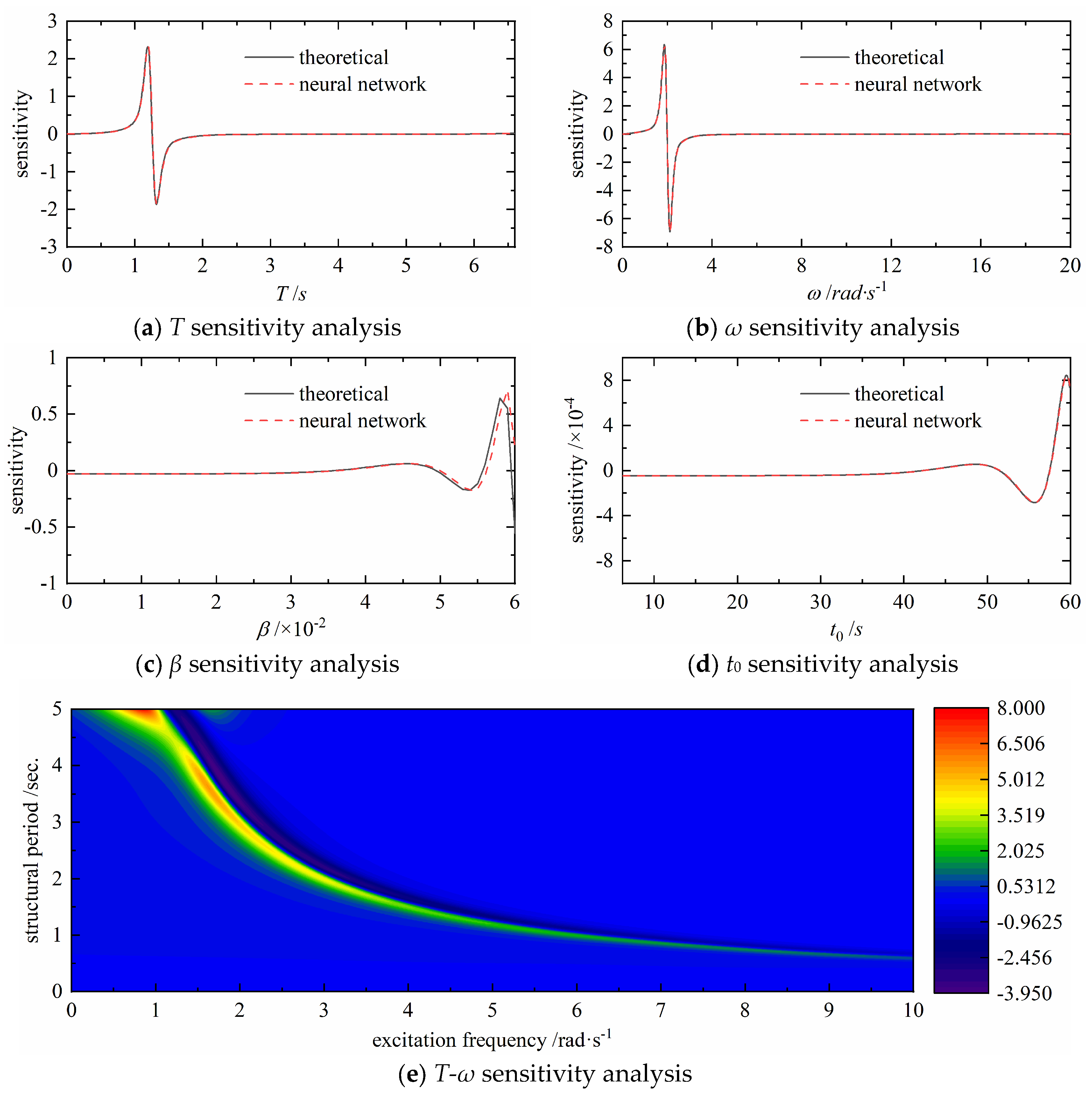
5.3. Analysis of Influence of the Parameters of the Intensity Non-Stationarity Based on Neural Networks

The BP neural network in this paper has three connection layers, of which the first two layers adopt hyperbolic tangent activation functions, and the output layer adopts linear transfer activation function. Equation (17) can be obtained by the chained derivation formula in Equation (16).

$$\begin{array}{cc}\hfill S_{\left(0,i\right),\left(3,1\right)}& =\frac{\partial x_{0,1}}{\partial y_{0,1}}\left[{\displaystyle \sum _{j=1}^{16}{\displaystyle \sum _{k=1}^8\frac{\partial x_{1,j}}{\partial x_{0,i}}\frac{\partial x_{2,k}}{\partial x_{1,j}}\frac{\partial x_{3,1}}{\partial x_{2,k}}}}\right]\frac{\partial y_{3,1}}{\partial x_{3,1}}\hfill \\ & =\frac{\partial x_{0,1}}{\partial y_{0,1}}\frac{\partial y_{3,1}}{\partial x_{3,1}}{\displaystyle \sum _{j=1}^{16}{\displaystyle \sum _{k=1}^8\left\{\left[\left(1-x_{1,j}^2\right)W_{0,i,j}\right]\left[\left(1-x_{2,k}^2\right)W_{1,j,k}\right]W_{2,k,1}\right\}}}\hfill \\ \hfill i& =1,2,3,4\hfill \end{array}$$

(17)

where y_0,1 and x_0,1 are the data values before and after the normalization of the ith input, respectively, and the normalization formula is shown in Equation (5); y_3,1 and x_3,1 are the output data values before and after the normalization, respectively, and the normalization formula is shown in Equation (6); W_0,i,j is the weight from the ith neuron at the input layer to the jth neuron at the first hidden layer; W_1,j,k is the weight from the jth neuron at the first hidden layer to the kth neuron at the second hidden layer; and W_2,k,1 is the weight from the kth neuron at the second hidden layer to the first neuron at the output layer. According to the normalization formula of the input and output data, the first two differential terms in Equation (17) are as follows:

$$\begin{array}{l}\frac{\partial x_{0,1}}{\partial y_{0,1}}=\frac{m-n}{y_{0,i,\max }-y_{0,i,\min }}\\ \frac{\partial y_{3,1}}{\partial x_{3,1}}=\frac{\left[\log \left(y_{3,1,\max }\right)-\log \left(y_{3,1,\min }\right)\right]\ln 10}{m-n}\times {10}^{\left\{\frac{\left(x_{3,1}-n\right)\left[\log \left(y_{3,1,\max }\right)-\log \left(y_{3,1,\min }\right)\right]}{m-n}+\log \left(y_{3,1,\min }\right)\right\}}\end{array}$$

(18)

where y_0,i,max and y_0,i,min are the maximum and minimum values before the normalization of the ith input data, respectively; y_3,1,max and y_3,1,min are the maximum and minimum values before the normalization of the output data, respectively; and m and n are the maximum and minimum values of the linear normalization, which are set to 1 and −1, respectively, in this paper. The data in Figure 8 are substituted into Equation (18), and the corresponding sensitivity analysis figures can be obtained, as shown in Figure 10.

According to Figure 10c,d, excitation shape parameter (β) and time of peak (t₀) have the least effect on the maximum absolute displacement response; the sensitivity of structural period and excitation frequency is first positive and then negative, which is consistent with the change rule of the structural response (which first increases and then decreases) near the resonance frequency. A similar rule can also be found is Figure 10e: when the structural period and excitation frequency are similar, the greater the sensitivity is and the higher the excitation frequency is, the smaller the effect of the vibration input on the dynamic response will be.

6. Conclusions

The effect of the intensity non-stationarity of ground motions on the structural dynamic responses is one of the scientific problems in the anti-seismic field. In this paper, the adoption of GA-BP neural networks in the research of the presented problem is proposed for the first time. Firstly, the initial weights and biases of the BP neural network are optimized by the genetic algorithm based on a small amount of training data. Then, the BP neural network is trained on all training data. Finally, the effect rule of the intensity non-stationarity of ground motions on the structural dynamic responses is obtained by studying the relationship between the BP neural network input and output. The main conclusions in this research are as follows:

(1) The GA-BP neural network in this paper, after trained with many data, can predict the maximum displacement response of the structure through four input parameters (time of peak t₀, excitation shape parameter β, excitation frequency ω, and structural period T). The results show that the GA-BP neural network has high prediction accuracy, but the high prediction accuracy can only be ensured within a certain range due to the limited range of training data. However, due to the generalization ability of BP neural networks, the range is larger than that of the training data.

(2) The sensitivity of the neural networks can be defined as the derivative of the output with respect to the input, which is used to measure the effect of the input change on the output. The analytical expression of the output of the BP neural network with respect to the input is obtained by mathematical derivation, and its comparison with theoretical value shows that the sensitivity from the calculation of the neural network is consistent with the theoretical value within the range of prediction accuracy. The results of the sensitivity analysis show that the maximum displacement output is the most sensitive to changes of the structural period and excitation frequency near the point of resonance.

(3) In the research on the effects of the nonstationary characteristics on the structural dynamic responses, compared with the analytic derivation method, the method based on the GA-BP neural networks can not only ensure the equivalent accuracy, but also avoid situations where the expression is too complex to solve; thus, this method can be extended to the study on the effect rule of nonlinear responses. Compared with numerical methods, the method in this paper can make full use of the advantages of neural networks in high dimension strong nonlinear fitting and comprehensively consider the effect rule of multiple input parameters.

References

1. Shinozuka, M.; Sata, Y. Simulation of nonstationary random process. J. Eng. Mech. Div. 1967, 93, 11–40. [Google Scholar] [CrossRef]
2. Iyengar, R.N. A non-stationary random process for earthquake. Bull. Seis. Soc. Am. 1969, 59, 1163–1188. [Google Scholar]
3. Hu, Y.; Zhou, X. Reactions of Elastic System Under Stationary and Nonstationary Ground Motions: Collection of Earthquake Engineering Research Reports (Episode 1); Science Press: Beijing, China, 1962. [Google Scholar]
4. Goto, H.; Toki, K. Structural response to nonstationary random excitation. In Proceedings of the Fourth World Conference on Earthquake Engineering, Santiago, Chile, 13–18 January 1969. [Google Scholar]
5. Amin, M.; Ang, A.H.S. Non-stationary stochastic model of earthquake motion. J. Eng. Mech. Div. ASCE 1968, 94, 559–583. [Google Scholar] [CrossRef]
6. Huo, J.; Hu, Y.; Feng, Q. Study on envelope function of acceleration time history. Earthq. Eng. Eng. Vib. 1991, 1, 1–12. [Google Scholar]
7. Qu, T.; Wang, J.; Wang, Q. Research on the characteristics of intensity envelope function of ground motions on local site. Earthq. Eng. Eng. Vib. 1994, 3, 68–80. [Google Scholar]
8. Du, D.; Wang, S.; Kong, C. Research on the three-dimensional earthquake non-stationarity model based on KiK-net strong motion records. China Civil. Eng. J. 2017, 50, 72–80. [Google Scholar]
9. Liu, X.; Yu, R. Analysis of approximate quantitative relationship between intensity nonstationary characteristic parameters of ground motions and structural responses. Earthq. Sci. 2016, 38, 924–933. [Google Scholar]
10. Jiang, H.; Du, D.; Wang, S.; Li, W. Effects of intensity nonstationary characteristics on structural dynamic responses based on damped-sine function model. J. Nanjing Tech. Univ. 2017, 39, 96–101. [Google Scholar]
11. Yao, X. Evolving Artificial Neural Networks. IEEE 1999, 87, 1423–1447. [Google Scholar]
12. Kitano, H. Empirical studies on the speed of convergence of neural networks training using genetic algorithms. In Proceedings of the Eighth National Conference on Artificial Intelligence, Boston, MA, USA, 28 July–1 August 1990; pp. 789–795. [Google Scholar]
13. Hancock, P. Genetic algorithms and permutation problems: A comparison of Recombination operators for neural net structure specification. In Proceedings of the International Workshop on Combinations of Genetic Algorithms & Neural networks, Baltimore, MD, USA, 6 June 1992. [Google Scholar]
14. Montana, D.J.; Davis, L. Training feedforward neural networks using genetic algorithms. In Proceedings of the Eleventh International Joint Conference on Artificial Intelligence, Detroit, MI, USA, 20–25 August 1989. [Google Scholar]
15. Peng, J.; Lu, W.L.; Xing, H.; Wu, X. Temperature compensation of humidity sensor based on modified GA-BP neural networks. Instrumentation 2013, 34, 153–160. [Google Scholar]
16. Liu, H.; Zhao, C.; Li, X.; Wang, Y.; Guo, C. Research on neural networks optimization algorithm based on modified genetic algorithm. Instrumentation 2016, 37, 1573–1580. [Google Scholar]
17. Engelbrecht, A.P.; Cloete, I.; Zurada, J.M. Determining the significance of input parameters using sensitivity analysis. Lect. Notes Comput. Sci. 2006, 930, 382–388. [Google Scholar]
18. Zhao, Q.; Ji, L. Finite element-neural networks hybrid method for parameter sensitivity analysis. China Civil. Eng. J. 2004, 37, 60–63. [Google Scholar]
Figure 1. Intensity nonstationary model based on the damped sine function.
Buildings 11 00069 g001
Figure 2. Algorithm flowchart of GA-BP.
Buildings 11 00069 g002
Figure 3. Schematic diagram of the artificial neural network.
Buildings 11 00069 g003
Figure 4. Comparison of histograms before and after the data normalization.
Buildings 11 00069 g004
Figure 5. Real-number coding of the chromosome.
Buildings 11 00069 g005
Figure 6. The evolution of fitness function.
Buildings 11 00069 g006
Figure 7. Validation of the trained artificial neural networks.
Buildings 11 00069 g007
Figure 8. Validation of artificial neural networks with single changing parameter.
Buildings 11 00069 g008
Figure 9. Structure of the artificial neural network.
Buildings 11 00069 g009
Figure 10. Sensitivity analysis of input parameters.
Buildings 11 00069 g010