Article

Evaluation of Metaheuristic-Based Methods for Optimization of Truss Structures via Various Algorithms and Lèvy Flight Modification

Department of Civil Engineering, Istanbul University–Cerrahpaşa, 34320 Istanbul, Turkey
*
Author to whom correspondence should be addressed.
Buildings 2021, 11(2), 49; https://doi.org/10.3390/buildings11020049
Submission received: 29 December 2020 / Revised: 26 January 2021 / Accepted: 29 January 2021 / Published: 31 January 2021

Abstract

:
Truss structures are one of the major civil engineering members studied in the optimization research area. In this area, various optimization applications such as topology, size, cost, weight, material usage, etc., can be conducted for different truss structure types. In this scope with the present study, various optimization processes were carried out concerning two different large-scale space trusses to minimize the structural weight. According to this state, three structural models provided via two different truss structures, including 25 bar and 72 bar truss models, were handled for evaluation of six different metaheuristics together with the modification of Lèvy flight for three of the algorithms using swarm intelligence by considering both constant and variable populations, and different ranges for iterations, too. Additionally, the effects of the Lèvy flight function and whether it is successful or not in terms of the target of optimization were also investigated by comparing with some documented studies. In this regard, some statistical calculations were also realized to evaluate the optimization method performance and detection of optimum values for any data stably and successfully. According to the results, the Jaya algorithm can handle the optimization process successfully, including the case, without grouping truss members. The positive effect of Lèvy flight on swarm-based algorithms can be seen especially for the gray wolf algorithm.

1. Introduction

In civil engineering, the most significant issue is to provide the required safety for any engineering structure. Of course, this state must be actualized by designers or engineers without putting people’s lives in danger; besides, the design must be cost-effective and also sustainable for eco-friendly structures and their members. However, to actualize this is not so fast and easy because of the desired and expected conditions that may not be able to be provided at the same time and with only a single step. On the other respect, the results obtained may not suitable or enough economic for the required conditions. For this reason, iterative processes, which benefit from both determining an optimistic design in terms of cost, effort, etc., and prevent spending much time, gain importance. From the past to nowadays, metaheuristic algorithms, which came as one of the optimization techniques and have been improved in the direction of some special features sourced on nature or science, are one of the best methods that can be selected for the mentioned state.
In this regard, several applications were performed via a wide range of metaheuristics in civil engineering, especially for structural engineering. As an example, in 2013, a study was carried out that is concerned with the generation of the best-tuned mass damper (TMD) parameters for structures. In the mentioned study, analyses were operated under different historical earthquake conditions by using harmony search (HS) algorithm to make real of this [1]. Parcianello et al. (2017) improved the viscous damper model for the frames depending on an optimization process conducted with genetic algorithms (GA) to increase of seismic performance of these structures [2]. On the other hand, Talatahari et al. (2015) developed a hybrid optimization tool by using eagle strategy (ES) and differential evolution (DE) algorithms to minimize the weight for different steel frame structures [3]. In addition, they evaluated the optimization success of this algorithm compared with DE. Gholizadeh and Ebadijalal (2018) benefited from a recently developed metaheuristic algorithm, which is named as center of mass optimization (CMO), to optimally arrange bracings on steel frames under seismic loading [4]. With the other respect, weight minimization of eccentrically braced frames was performed in the direction of seismic performance-based analysis by Fathali et al. (2020). Four algorithms, including accelerated water evaporation optimization (AWEO), PSO, with classical (CBO) and enhanced (ECBO) colliding bodies optimization, were utilized to observe the performance of this method [5]. Moreover, Kayabekir et al. (2016) presented a book where optimum designs were generated for reinforced concrete structures containing slender columns, shear walls, and cylindrical walls formed as post-tensioned axially symmetric, etc., through the usage of metaheuristic algorithms [6]. Vaez and Qomi (2018) carried out a study, which is related to providing minimum weight for reinforced concrete shear walls by investigating the optimum placement and diameter of steel bars together with wall properties by using PSO, FA, whale optimization algorithm (WOA), and crow search algorithm (CSA) [7]. In the study performed by Sheikholeslami et al. (2016), two metaheuristics, including firefly algorithm and harmony search, were hybridized and applied to two different reinforced concrete retaining walls to provide the best cost [8]. Optimum design for a cantilever retaining wall was also carried out with the aim of cost minimization by Aydogdu (2017), where peak ground acceleration was considered towards this object by combining of biogeography-based optimization method with Lèvy flight [9]. Additionally, the design of retaining wall with the optimum cost was realized depend on seismically performance based by handling an enhanced kind of genetic algorithm (non-dominated sorting).
Similarly, various optimization studies were also performed for truss structures too. One of these is a study, which was carried out to provide the minimum weight for space truss structures by Camp (2007) through using the big bang–big crunch (BB–BC) optimization algorithm [10]. While executing this process, deflection and stress limitations besides material conditions were considered. In the year 2011, another study was performed for trusses in the direction of minimization of structure mass by providing of optimum size and shape of them [11]. To make real of this, an optimization technique, which is one of the oldest and called particle swarm optimization (PSO), was utilized, and it was applied for four different structure models. Moreover, Miguel and Miguel (2012) carried out a work which is related to optimization of shape and size of trusses by using nodal coordinates and section areas of bars, respectively, to reach minimum weight [12]. For this aim, they used two optimization tools, including the firefly algorithm (FA) and harmony search (HS), for analyzing four different truss models. In 2015, Bekdaş et al. (2015) applied a metaheuristic known as flower pollination algorithm (FPA) to generate the best truss size by minimizing structure weight, and they used three truss models containing planar and space form to actualize this process [13]. On the other hand, Kaveh and Ghazaan (2017) used a metaheuristic algorithm to optimize truss structures to improve the dynamic performance of them under frequency constraints [14]. For this reason, they benefited from a method, which is known as vibrating particles systems (VPS), and was developed by inspiring from dynamic behavior of structures. Tejani et al. (2018) also solved the problem related to multiobjective optimization of five different truss structure models from the literature [15]. In this respect, they applied the symbiotic organisms search (SOS) algorithm by combining the multiobjective adaptive control technique.
The widest application area of metaheuristic-based optimization is truss structures in structural engineering. Furthermore, in Table 1, a comparison is carried out by generating a summarization of optimization properties about some literature studies, which are benefited from the validation of the present results. The current study and compared documented methods are compared to each other in terms of the variety of the number of the used algorithms, the number of design variables, etc.
In the current study, two different space truss structure models as 25 bar and 72 bar that are generally used as the benchmark problems, were handled to ensure optimum design parameters, including section areas and also objective functions such as minimum cost or weight, etc. In this regard, three separate cases were emphasized by considering the numbers of increment of design parameters. According to this, the first and second one is related to combining/grouping of structure bars for truss models, besides that, the last is the case, where grouping for the 25 bar model is not realized. Six different metaheuristic algorithms and three improved versions of them using Lèvy flight as a novel application were applied to the mentioned cases by generating two sub-cases of different maximum iteration and population numbers. As given in Table 1, the present study includes the application of 9 algorithms with three novel modifications. In addition to that, a comparative investigation using nine applied methods and seven documented methods was presented by choosing the same optimum design benchmark problems.

2. Materials and Methods

When the general of nature is considered, it is understood that livings have features developed for various aims such as surviving, feeding, continuity of species. To see these features, many examples such as that fox benefits from a magnetic area of the world while it is hunting, chameleon changes color intending to hide from danger; cuckoo birds use other bird’s nests for continuity of self-species and hedgehog throws the quills by stretching itself under danger, are possible. If when all these processes are analyzed, it is seen that livings change their defense or attack mechanisms as conveniently to the conditions and uses a kind of species-specific heuristic optimization, which ensures that using of limited opportunities exist in themselves under the fittest time and form to maintain of vital activities.
These heuristic optimization processes belonging to livings in nature have engaged the attention of researchers working on basic sciences, and they generated various algorithms, which express these processes mathematically as the most frequently and commonly used in the literature from these algorithms called metaheuristics are explained in headings taken below and employed in the study.
The employed algorithms are flower pollination algorithm (FPA), artificial bee colony (ABC) algorithm, bat algorithm (BA), Jaya algorithm (JA), gray wolf optimization (GWO) and harmony search (HS). These algorithms have unique features and imitations from a process. These are detailly explained in the subsections of Section 2, but major generations and differentiation are as follows:
-
FPA, ABC, BA and GWO are nature-inspired algorithms. HS is a music-inspired one, while JA does not use a direct imitation. Jaya word means victory in Sanskrit. Due to that, a bond can be only generated by assuming the reaching of an optimum result as a victory;
-
FPA uses Lèvy distribution in its classical form. Since wolves, bees and bats can also act as random flying or moving members, modified versions of these algorithms with Lèvy distribution that characterize the random flight are investigated;
-
Generally, metaheuristic algorithms have two stages of optimization using a probability to select one of these stages (phases) in an iteration. ABC is a three-stage (phase) algorithm, while JA has only a single phase. The others are classical two-phase algorithms;
-
JA has no user-defined specific parameter in the formulation, while the others need parameters in formulations and selection of a stage;
-
BA uses a three-step formulation (frequency, velocity and new solution) to update a solution.
-
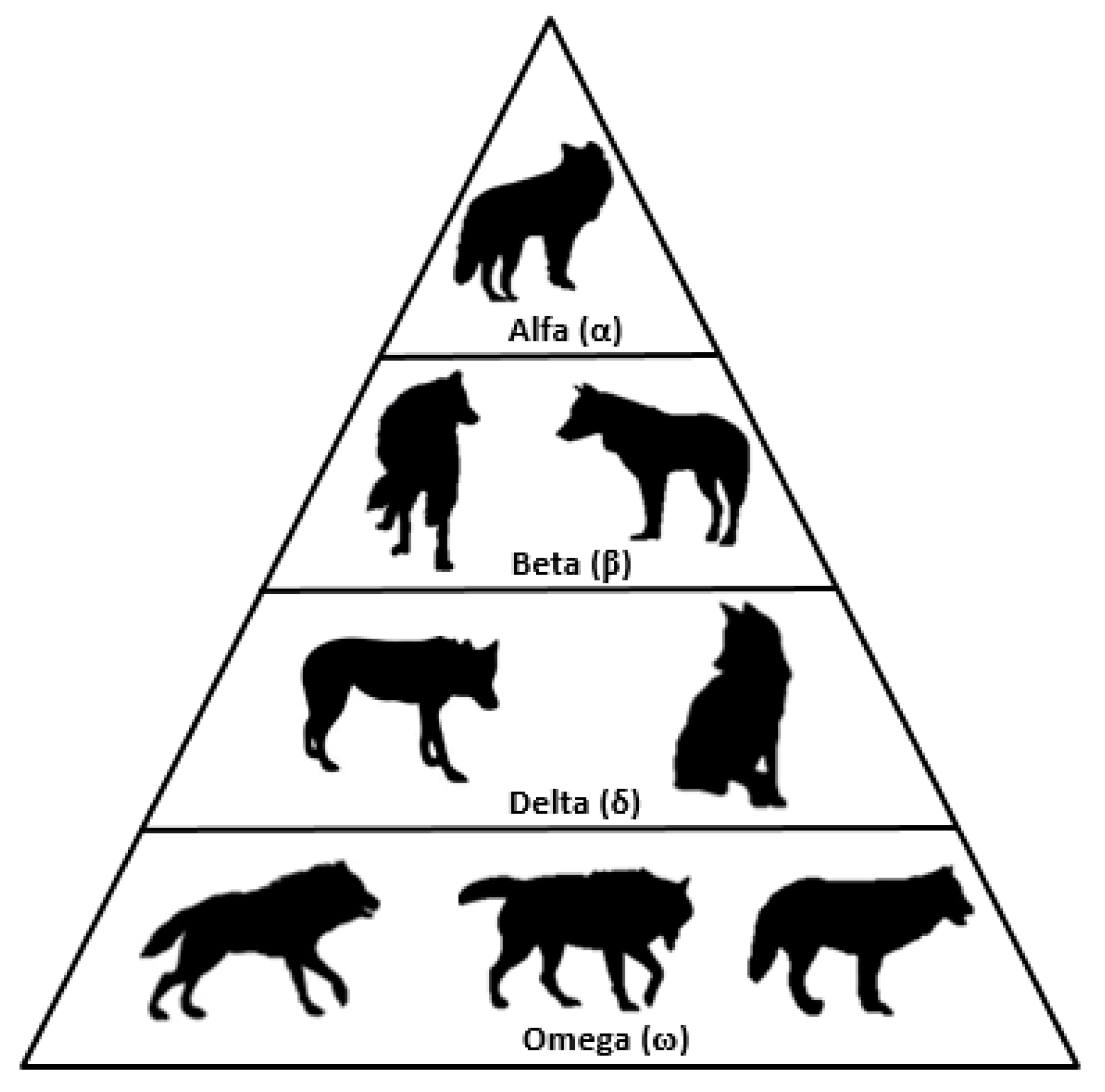
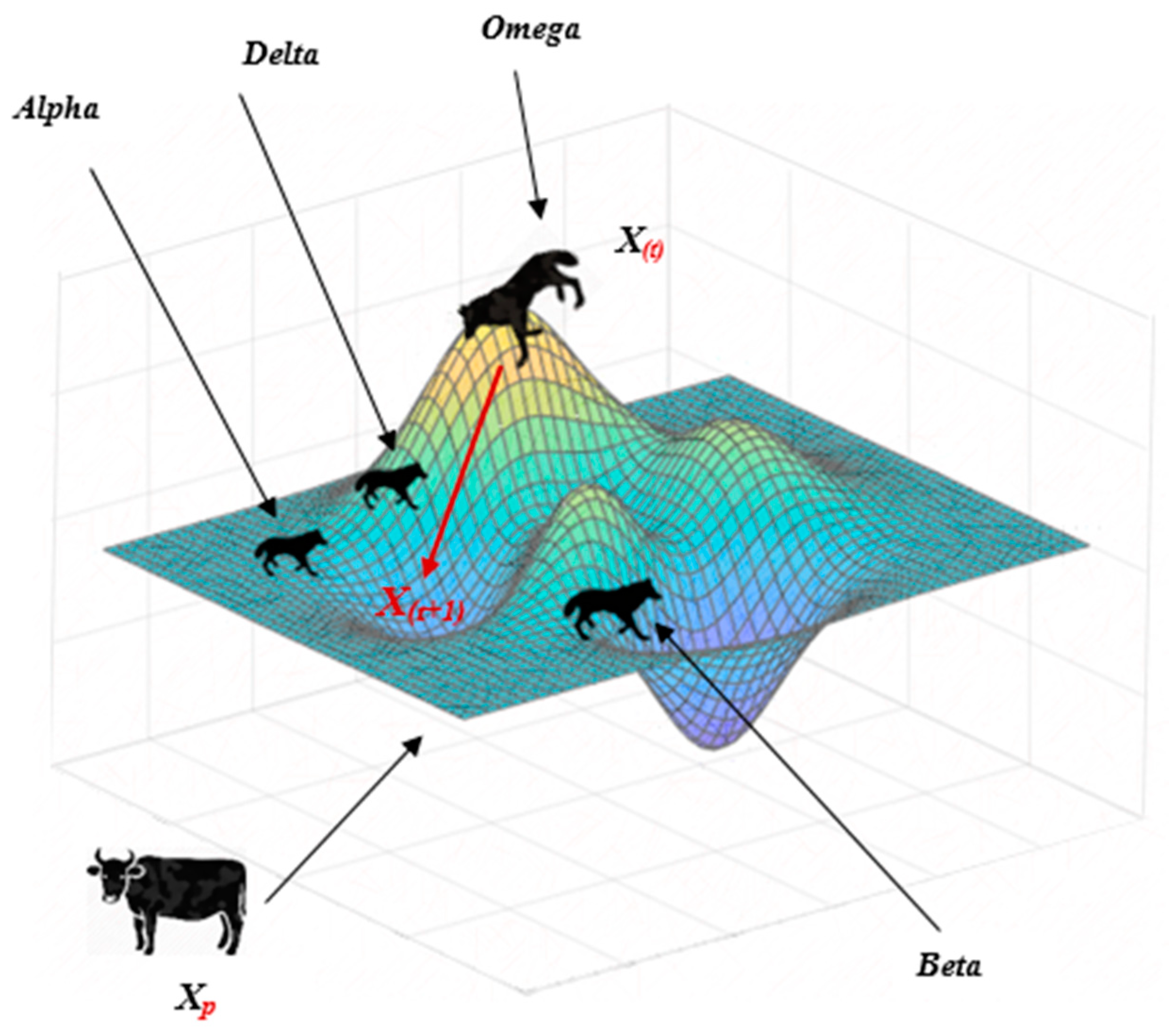
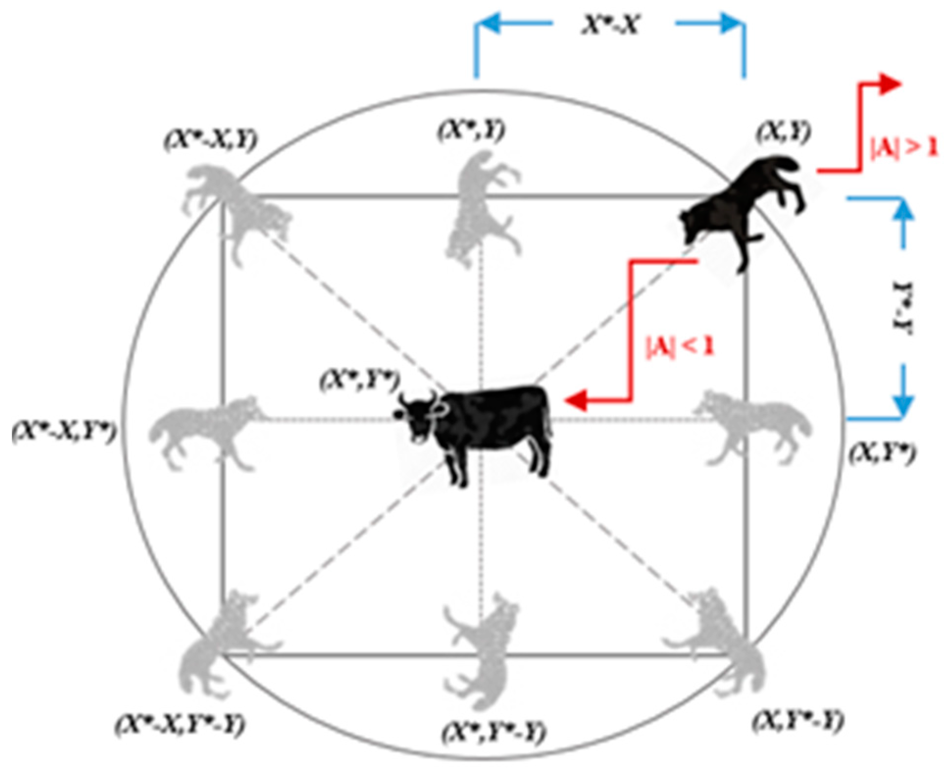
GWO uses three unique, different solutions with different calculations. These solutions are named with three types of wolves.
In Appendix A, the commonly used type-specific parameters belonging to each metaheuristic method and some common expressions concerned with candidate solutions for each design variable can be seen. In addition, the used functions in equations of algorithm optimizations are indicated in Appendix A.

2.1. Flower Pollination Algorithm (FPA)

Plants, especially flowering plants, can gain attract to self of some insect species like bees, flies, etc., because of that they have stimuli such as special color, smell and various aromatic secretories. In addition to these features, insects also contribute to the pollination process, which is required for ensuring the continuity of species by the run to flowers with the help of nature-sourced effects like wind, water, etc.
The flower pollination algorithm (FPA), which was developed by inspiration from this process by Yang [25], is one of the metaheuristic algorithms frequently used nowadays. In FPA, four different rules, which are related to the property of pollination process, the behavior of pollination, and flower constancy, and formalized by inspired from flowery plants, are kept insight [13,26,27]:
  • Cross-pollination is realized via the transfer of pollen between flowers of different plants from the same species. Pollen carriers (pollinators) suit to rules Lèvy distribution (Equation (1)) by jump with far steps or fly. This process is called global pollination;
  • Self-pollination occurs due to the pollen transferring within the self of a flower or between different flowers of the same plant. This pollination kind is local pollination;
  • The case of flower constancy is the cooperation among pollen carriers with flower types. This is a development within the process of flower pollination;
  • Local and global pollination is controlled with a probability value, which is named switch probability and has a value between 0 and 1.
In the optimization process, which is performed via applying all these rules, two different ways are followed to obtain the optimum values. To make real this, the type of search must be determined by controlling search change/switch probability ( sp . ), which is one of the FPA parameters. This search type is named as:
  • The global search that solutions are determined by search from more extent area, if sp is bigger than a randomly generated number;
  • The local search process that solutions are searched from a smaller area if this value sp is smaller than the generated random number between 0 and 1 (rand).
The value of the ith design variable of the jth value of population including nf number of flowers ( X i , j ) is updated as the new solution ( X i ,   new   ) as given below. X i , g best is the best current solution of the ith design variable.
L é v y = ( 1 2 π ) ( rand ) 1.5   e ( 1 2   rand     )
X i ,   new   = { sp > rand ,                     X i , j + L é v y   ( X i , g best X i , j )   sp < rand ,   X i , j + rand   ( X i , m X i , n )
n = ceil   ( rand   ×   n f )
m = ceil   ( rand   ×   n f )

2.2. Artificial Bee Colony (ABC) Algorithm

In 2005, the artificial bee colony (ABC) algorithm introduced by Karaboğa was developed through simulated the food source searching behaviors of bee colonies [28].
In bee colonies, honey bees are divided into three different categories as a worker, onlooker, and scout. Moreover, in the algorithm, these categories represent the negative feedback, positive feedback, and random motions, respectively. Initial food sources are produced randomly in the search space of the problem. Half of the honeybees that have the aim to provide the increase of the substantiality of nectar in the hive are worker bees. The other half contains onlooker bees, and flocking behavior around the food source starts with worker bees. Worker bees record each food source to the memories, and information is shared with onlooker bees waiting in the hive. According to shared information, onlooker bees collect the food sources within the near-environment of the hive; scout bees collect the ones in long-distance from the hive. Onlooker and scout bees share the food source information with worker bees by a return to the hive. If the information on the new food source is better than the information on the initial food source’s position, this is updated [29,30,31].
In this way, the ABC algorithm can deliver a solution to various optimization problems thanks to the simulation with the natural process, which is the maximization of nectar amount by determining the position of food sources optimally by honey bees.
Some assumptions are applied in this algorithm, too [32]. These are given below:
  • It is accepted that number of worker and onlooker bees are equal to each other in the total bee population;
  • The food sources express candidate solutions and are assumed that each bee completely consumes this source by going to a single food source. Hence, the food source number is half of the total bee number;
  • Later, worker bees transform into scout bees to search for the new ones substituted for finished foods.
There are four separate stages for expressing this process via the ABC algorithm. These are determining of initial food sources, the worker bee stage that found of the new sources by worker bees, onlooker bee stage that evaluated nectar qualities of new sources, and finally, scout bee stages that found the new ones, in the case that exist finished food.
About improving initial food sources, first, the worker bee stage is performed. For this; one food source is selected as randomly ( n ), and the position of the old source is updated with a probability value ( ϕ i , j ) between the range of [−1, 1] for a design variable/parameter determined randomly ( p ) for a problem with vn design variables/parameters, and source nectars are calculated again. From sources that their positions were updated, all of the food sources that are better than the initial ones are updated by changed with the old food source. This process for modification of the design variable of the jth population ( X p , j ) is carried out via equations expressed below:
X p , new = X p , j + ϕ i , j   ( X p , j X p , n )
n = ceil   ( rand   ×   e b )
p = ceil   ( 1 + ( v n 1 )   rand )
The second stage is the onlooker bee stage. In this stage, onlooker bees are kept informed by worker bees with regards to food sources’ nectar amount. The food quality/rate/possibility according to the nectar amount of each source is calculated and evaluated by onlooker bees. This operation is related to the selection of ones, which have a high ratio of nectar from renewed food sources, and in this way, the sources, which are rich in nectar, are ensured the improvement of them as continuously by determined. In addition, this process is performed via Equation (8) in case that food possibility (Equation (9)) is bigger than a number randomly generating. n e c t a r j (Equation (10)) is quality value for jth food sources (candidate solution) calculated depending to the objective function and considering of problem type; F j is objective function value belonging jth solution and f o o d   p o s s i b i l i t y j is nectar rate existing in each source (rate of nectar quality):
if   rand < f o o d   p o s s i b i l i t y j ,   X p ,   new = X p , j + ϕ i , j   ( X p , j X p , n )
f o o d   p o s s i b i l i t y j   = n e c t a r j j = 1 f s n n e c t a r j
n e c t a r j = 1 1 + F j
The process of searching for new sources by abandoning sources that cannot be optimized (namely nectar of them) is named as scout bee stage. Improving parameter ( ip ) belonging to each source is controlled according to a constant value of source improvement limit ( SIL ), which is defined at the start of the optimization process to use in this stage. By scout bees, determination of new ones for each source that has ip values exceeding the value of SIL is realized utilizing Equation (11) as below for the defined maximum ( X i , max ) and minimum ( X i , min ) values. For modification with Lèvy distribution, the rand function is replaced with Equation (1).
if   ip J > SIL ,   X i , new = X i , min + rand   ( X i , max X i , min )

2.3. Bat Algorithm (BA)

Small bats known as micro bat perform echolocation behavior acting as a kind of radar to locate their prey, protect from obstacles, and can detect the place of hollows/clefts where they lived at night. These bats listen to echoes returning from objects by transmitting a very noisy sound. In addition, the frequency of transmitted sound shows alteration according to features of bats. Bat algorithm (BA), which is a metaheuristic method, is developed by Yang through be idealized of echolocation behavior and these features belonging to bats [33]. Furthermore, bats fly with variable frequency values, loudness, and velocity, which can be used in designing update equations of algorithms [27,34].
On the other hand, some assumptions are required to be able to use the BA algorithm in the optimization process, as in the other algorithm types [33,35]. These assumptions are as below:
  • All bats use audio echo to sense distance;
  • Bats move randomly at any X i   location via V i   velocity by using a sound, which has a constant frequency, variable λ wavelength, and loudness with A 0 value, to search for the prey. They can adjust the wavelength of emitted pulses or frequency automatically, and the pulse emission rate (r) depending on closeness to its target (r [0, 1]);
  • Although loudness value can change in different ways, this value changes between an extremely high (positive) initial value ( A 0 ) , and a constant minimum value ( A min ) . A 0 is 1 due to that bat search its prey with a very loud sound in the beginning; also, when it is considered that bat just found the prey, and abandons to giving out a sound as temporarily, A min can be taken as 0.
In the direction of these assumptions, it is required that each bat have different loudness and pulse emission value; besides, some different properties must observe for determining new values (locations) belonging to candidate solutions in the optimization process performing via the BA algorithm. These are frequency ( f j for the jth member with the minimum; f min and the maximum; f max ) and velocity vectors, and the process is carried out with equations as below, respectively:
f j = f min + ( f max f min ) rand
V i , new = V i , j + ( X i , j X i , g best )   f j
X i , new = X i , j + V i , new
An iterative replacement (update) is in question for new locations designated for bats (solution value of design variables). This replacement is a process called local search, and calculation is made with the help of Equation (15):
if     rand > r   j ,     X i , new =   X i , g best + ( 1 + 2 rand )   A mean
On the other hand, the values of loudness and pulse emission rate should be updated as long as iterations progressed. The reason for it is that distances of bats to foods or their prey change per the updated locations of bats. About this subject, generally, pulse emission rate increases according to a decrease of loudness when bat found the prey, according to the expression of Yang [33]. In this direction, parameters are updated along with iterations via Equations (16) and (17):
A   j , new = α   ( A min + ( A 0 A min ) rand )
r   j , new = r j 0   ( 1 e γ t )
In Appendix A, the calculated and utilized expressions for the optimization process were given except the commonly used expressions. In the Lèvy improved BA, the A mean value in Equation (15) is replaced with Equation (1).

2.4. Jaya Algorithm (JA)

Jaya algorithm, which is recently developed by Rao (2016), and has a working principle similar to the teaching-learning based optimization (TLBO), is one of the metaheuristic methods [36]. This algorithm always tries to be closer to the approach of being optimal. In this regard, the main targets of the algorithm are both reaching the best solution and moving away from the worst solution ( X i , g worst ). On the other hand, the algorithm takes the name from Jaya, which is a Sanskrit word, meaning victory. It is harmonious with this operation, and it is aimed to achieve optimization of the solution.
When the Jaya algorithm is compared with the other algorithms, generally, it evaluates fewer functions to obtain the best same result. For this reason, it is required fewer operations than others in the process of convergence to the ideal solution. However, the application of the algorithm is simple and also not including special parameters, which are considered superiorities [36]. However, the possibility that the algorithm locks to local optimum increases due to the algorithm searches the best and worst results around a smaller area compared to the other methods, and this case may cause to be not able to evaluate better results.
In each iteration, a single-stage is enough for all variables to obtain a new optimum solution. Equation (18) utilizing for this is as below:
X i ,   new   =   X i , j + rand ( X i , g best | X i , j | ) rand ( X i , g worst | X i , j | )

2.5. Gray Wolf Optimization (GWO)

Mirjalili et al. (2014) developed an algorithm, which is called gray wolf optimization (GWO), and it is a kind of metaheuristic optimization method by considering the hierarchy of leadership of gray wolves, which usually live in groups, and have hunting mechanism in real nature [37].
In nature, gray wolves, which underlie this algorithm, create groups containing 5–12 members on average. Wolves categorize into four different as alpha, beta, delta, and omega wolves due to the existence of hierarchy between themselves. Group leader named as the alpha wolf, has responsibilities such as hunting, determining of sleep place with waking time by managing the other wolves in the group, too. In this respect, it is required that the alpha wolf, which is in the leading position, is the best member in terms of managing the pack, not the strongest member. In addition, this shows that the case of organized and discipline keeping in the pack is more significant than power. Wolf at the second level of the hierarchy, is the beta wolf and participates in the group as the alpha wolf’s assistant in many respects. Moreover, when the case that alpha wolf dies or is at a very advanced age, the beta wolf is considered as the most possible member as a candidate, which will be able to replace. In the group, the main task of this wolf is both providing to keep informed of delta ( δ ) and omega ( ω ) wolves by transferring the instructions transmitted to the leader and giving their instructions to these wolves situated in lower level than itself by applying the directions taken from alpha. In the third and fourth steps of hierarchy, delta and omega, which are less strong wolves, respectively, and the delta wolf can gain an advantage over only omega wolves. For this reason, it can be said that the weakest member in the group is the omega wolf in terms of leadership/dominance. The representative demonstration of social hierarchy among gray wolves takes place in Figure 1 [38,39].
On the other hand, group hunting is a social behavior that gray wolves performed in real nature, and also, this natural behavior was benefited for algorithm design-oriented at optimization process. In this respect, first, the strongest three wolves need to be determined among wolves in the group. Here, the best three solutions set is determined from among each member in the initial wolf ensemble; in other words, candidate solutions, and alpha ( α ) as the leader-member (the best convenient member in terms of the objective function), the second strong member beta ( β ) and third one delta ( δ ) solutions are defined. All solutions except three candidate solutions are represented by the other wolves that remained in the pack, and these members are considered omega ( ω ) solutions. Hence, hunting behavior reflecting the optimization process is directed by α , β , and δ wolves. In addition, there is a certain order followed by wolves during hunting, and according to this order, first, the prey is followed, then encircled by wolves. In the meantime, D , which expresses the distance between prey and any wolf surrounding it, is calculated with Equation (19). Moreover, wolves can update their locations around the prey randomly, depending on prey (Equation (20)) [37,40]. In addition, for Lèvy modification of GWO, rand function existing in A vector formulation (Equation (22)) is changed via Equation (1):
D = | C   X i , pr X i , j |
X i , new = X i , pr A D
C = 2   rand
A = 2 a   rand a
a   = 2 2 t stopping   criteria
As mentioned before, the hunting process is directed by α, β, and δ wolves. Figure 2, which shows this case more clearly, takes in below. In this stage, hunting is performed by wolves attacking the surrounded prey. However, as seen in the figure, first, it is required that hunting be directed healthfully and determining of locations (according to the prey) of α , β and δ wolves that are assumed to have information well about the potential position of the prey. For this, the following equations are applied (Equations (24)–(29)), respectively:
D α = | C 1   X i , α X i , j |  
D β = | C 2   X i , β X i , j |  
D δ = | C 3   X i , δ X i , j |  
In these equations, D α , D β and D δ are the distance between any gray wolf and alpha, beta and delta wolves, respectively:
X i , α new = X i , α A 1   D α
X i , β new = X i , β A 2   D β  
X i , δ new = X i , δ A 3   D δ  
In the above equations, respectively, A and C vectors are expressed individually for alpha, beta and delta wolves, and the approximate distance between any omega ( ω ) wolf, namely the current solution, and α , β and δ wolves can be determined via Equations (27)–(29). The latest updated position of the current solution is calculated as in Equation (30):
X i , new = X i , α new + X i , β new + X i , δ new 3  
The wolf, which updates its position, is ready to attack prey. However, also, there are some rules about mathematically expressing the case that wolf can realize the attack. Accordingly, in this algorithm, the a   value was reduced for the wolf that can approach (decreasing of the distance between them) to prey. In addition, A   vector, which determines the case of attacking to prey by a wolf, utilizing this decreasing and take values between − a   and a   . Hence, the environment, which is taken place in the hunting process, can be expressed as in Figure 3. On the other hand, a new position of hunter wolf can take values between the position of prey and own current position. As a summary, the case that wolf can attack prey actualizes to the condition in Equation (31) [14,41]:
if     | A | < 1 ,   X i ,   new = X i , pr

2.6. Harmony Search (HS)

One of the aims of musicians while offering a musical performance to listeners is to transfer work euphoniously. For this reason, the process of creation of an effective and good music work through a combination of notes, which are the best reflecting the works and most harmonious each other, continues to gain the appreciation of listeners.
Geem et al. (2001) [42], who was inspired by this process, developed an algorithm in 2001, which is known as the harmony search (HS) method, and based on natural (impromptu) music performance. The aim is to search for the liked harmony [43]. The functioning of this developed algorithm is not only offering of a music work by melodizing via the best notes, at the same time, but it also takes shape according to natural performance of a musician and idea that to optimally implement while performing of this, too.
When analyzed this process, three possible activities, which can be performed during the natural performance of a musician, and equivalents of these in terms of actions realized by harmony search is [44]:
  • To play any popular musical piece completely from own memory: usage of harmony memory;
  • To play something like to a known work: pitch (tone) adjusting;
  • To compose/melodize new or random notes: randomization
Usage of memory is an important notion due to resembles case that of obtaining the best harmonies, which will transfer to new harmony memory, like selecting the most convenient persons in the genetic algorithms (GA). Here, a case that harmony memory consideration rate, which has a value between 0 and 1, is very high, causes to not finding out well of almost whole harmonies in old harmony memory [45].
Furthermore, on optimization of a problem, natural music performance can be considered as a process expressing that determining of optimum values for design variables. The most compatible notes/harmonies express the optimum values of design variables; the best, in other words, “most euphonic” music work, which occurs with the combination of these notes, expresses the case that performing of the objective function belonging to design problem.
The followed route by algorithm on optimization of design values changes according to the different cases. In each iteration, obtaining the optimized new values of variables is depending on the usage of harmony search memory. This case is determined via harmony memory consideration rate (HMCR) according to Equation (32).
  • If the HMCR value is bigger than a randomly generated number, memory usage is not possible. In this case, randomly new notes should be generated;
  • In the other case, notes recorded in harmony memory can be played from a specific pitch by remembering:
X i ,   new   = {   HMCR > rand ,     X i ,   min + rand   ( X i , max X i , min )   HMCR < rand ,     X i , n + rand ( 1 2 , 1 2 ) PAR   ( X i , max X i , min )  

2.7. The Benchmark Truss Structure Problems

In this study, two large-scale truss models were handled for optimum sizing of bar sections in the direction of weight minimization. These are represented in Figure 4 and Figure 5 as the geometry of 25 and 72 bar truss structures together with node and bar numbers in the space coordinate system, respectively.
In the optimization process, three cases were conducted to provide the minimum weight for these structures by the grouping of bars both 25 and 72 bar truss, and without grouping of 25 bar truss intended for evaluation of designing based on increment on the number of design variables. In this regard, design variables and constraints, which were determined by collecting in the same section area according to axis similarity and symmetry of bars for grouping cases, were given in Table 2. The material of the structures is aluminum. The same methodology can be applied for different materials, and design regulation rules can also be integrated as design constraints. Especially, the slenderness limits of the members under compressive forces are needed to be checked. In addition, the multiple loading conditions are in Table 3 and Table 4; design limitations as displacement and stress constraints with bar groups are in Table 5 and Table 6, for 25 and 72 bar trusses, respectively. The optimum results for all cases were ensured without permitted the violation of any constraint through penalizing the solutions, which exceed the limitations.
On the other hand, when performing optimization, six different metaheuristics containing HS, ABC, BA, FPA, GWO, and JA, besides ABCL, BAL and GWOL, were applied by modifying the structure of three algorithms with Lévy distribution. Additionally, optimization results, including the best weight together optimal section areas, were determined to a specific population number as 30 and different iteration numbers. Following, for grouping cases (Section 3.1 and Section 3.2), the values of optimization parameters were handled in the range of 10–30 with 5 intervals and 1000–20,000 by increasing 500; and in not grouping case for 25 bar truss (Section 3.3), the same ranges, and 5000–120,000 by increasing 5000 for population and iteration numbers, respectively, to detect the most effective parameters in the sense of saving time and effort during that minimum weight was determined.

3. Numerical Examples

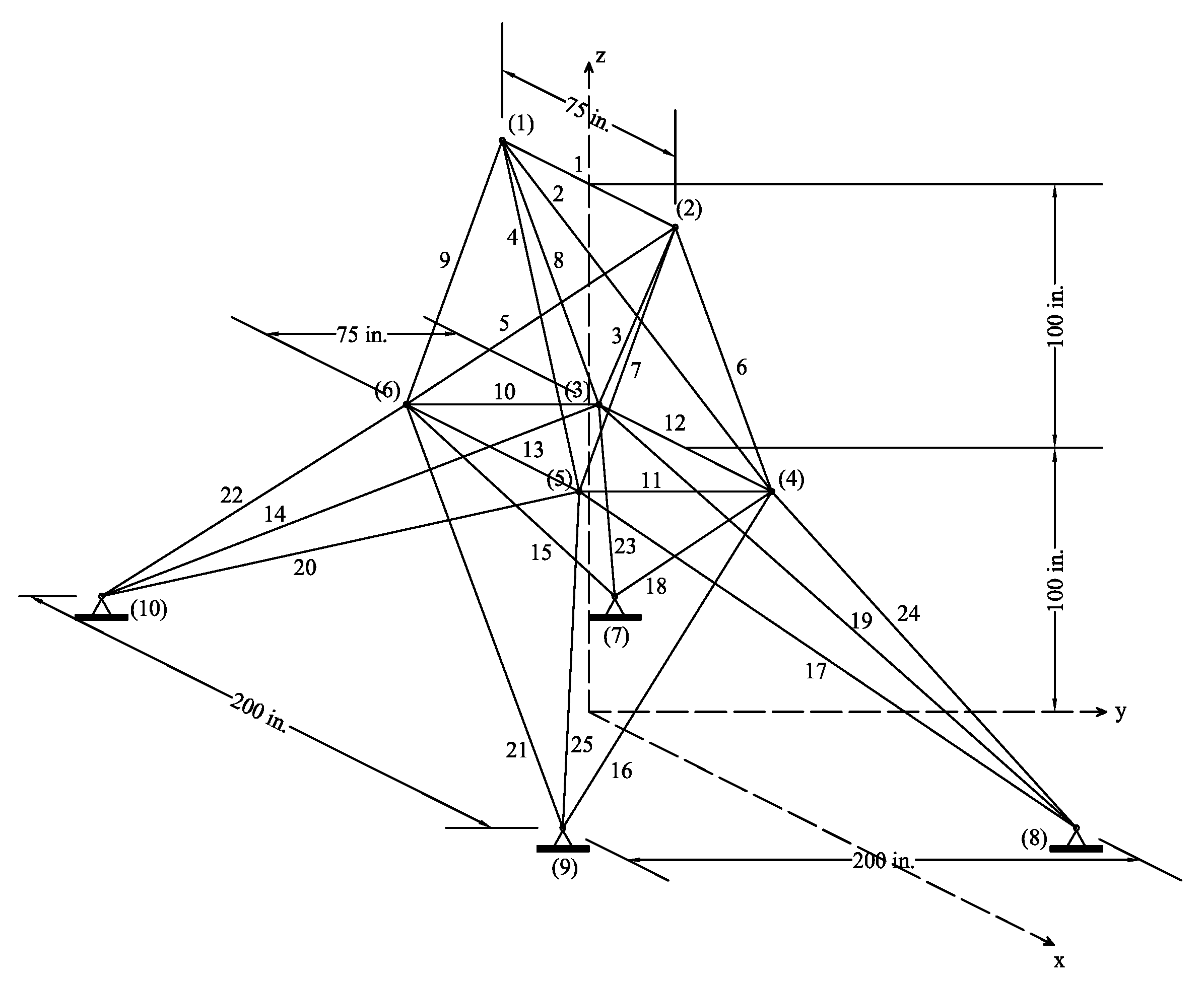
3.1. 25-Bar Truss Optimization with Bar Grouping

The first case is an application performed for 25 bar truss sizing optimization by the grouping of whole bars. To realize this, bars were assigned to specific section areas by collecting similar ones symmetrically according to axes in the spaceplane. While performing the optimization process, the aforementioned stages were applied as the usage of a constant population number as 30 together with different iteration numbers that can be seen in Figure 6. Moreover, several populations and iteration numbers were interworked. The minimum weight is obtained as 545.0413 lb through JA in 20,000 iterations.
In addition to this, optimization results of some literature studies were given in Table 7 to evaluate and compare the results found by used algorithms currently. In addition, in Table 8, the results, including minimum weight and statistical calculations, and optimum design variables, can be seen for each metaheuristic. As it is understood from these tables, the most successful algorithm is JA due to be able to determine the minimum weight with a very small standard deviation. Moreover, JA and FPA with the usage of Lèvy distribution by nature outperform the compared literature results in the best optimum value. It is seen that the Lèvy distribution has a positive effect on the best and mean optimum values.

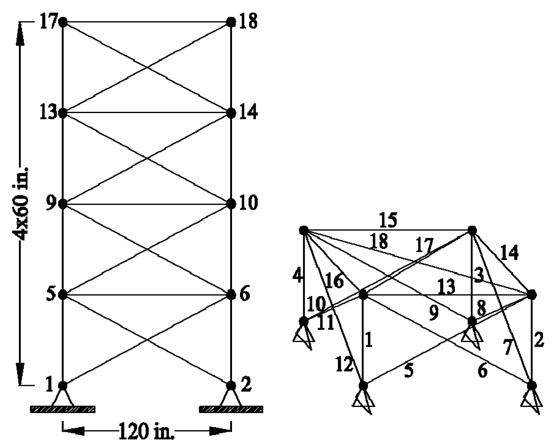
3.2. 72-Bar Truss Optimization with Bar Grouping

The second case is the grouping of bars belonging 72 bar truss to provide optimal design variables and the best weight solution. In Figure 7, optimization results as minimum weight (379.6172 lb via JA in 15,000 iterations) are presented that they were obtained according to the constant population and various iteration numbers.
In Table 9, all current optimization results were represented with some parameter evaluations. Literature studies are also given in Table 10. For this case, the best metaheuristic is again JA owing to reach the minimum weight, which is a far smaller value than the other algorithms. Furthermore, according to this algorithm, the standard deviation for the objective function is very little and so that it can be recognized that JA has the best performance in every respect when the other current methods and the used previous algorithms are compared.

3.3. 25-Bar Truss Optimization without Bar Grouping

The third case is concerned with the determination of optimal section areas for each bar individually. In this regard, the best weight as a minimum (545.1083 lb) was achieved with JA by considering the only constant population in 100,000 iterations, as seen in Figure 8. In addition, it was understood that the objective function might be provided by usage of the best parameter combinations as 15 and 115,000 for population and iteration numbers with JA, respectively, according to the results of Table 11. For this case, the only documented optimization was proposed by Bekdaş et al. [24].

4. Results

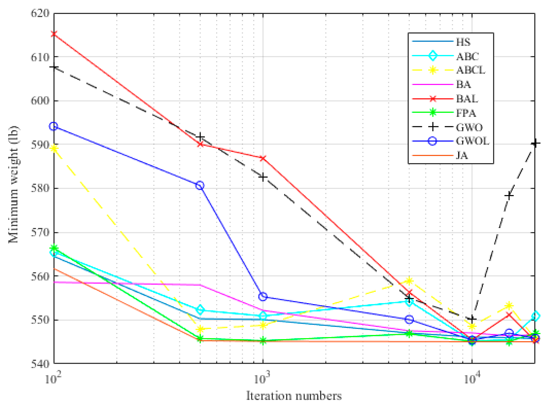
4.1. 25-Bar Truss Optimization with Bar Grouping

As it was mentioned previously, first, an optimization operation was applied by utilizing a constant population and different iterations (Figure 6). Generally, it can be recognized from this figure, all of the ones can be considered as successful except GWO, ABCL, and BA in terms of nearing the minimum weight. However, in this meaning, the best algorithm is JA, thanks to the finding of weight as 545.041 lb at minimum. Nevertheless, Lèvy flight is effective for both BA and especially GWO.
On the other respect, according to the results in Table 6 and Table 7, from the used algorithms in the current applications, JA is the method that can find the minimum weight as 545.0378 lb, which is a smaller value than the best one from literature studies, and it was provided with an extremely small deviation. Additionally, except for JA, it appeared that FPA could also be accepted as accomplish for minimization of the weight according to the given literature results. Thus, this algorithm employing Lèvy distribution in its initial form can be minded as effective and useful due to that it can achieve this objective by making little standard error. If we evaluate the other methods, it can be said that GWOL and BAL almost approximate to the minimum weight for grouping case of the 25 bar truss. Here, the significant point is that Lèvy flight is noteworthily effective in terms of minimizing of weight by all of the swarm intelligence-based algorithms, especially for GWO, besides that the required iteration numbers were decreased with this function for BA and especially ABC, too.

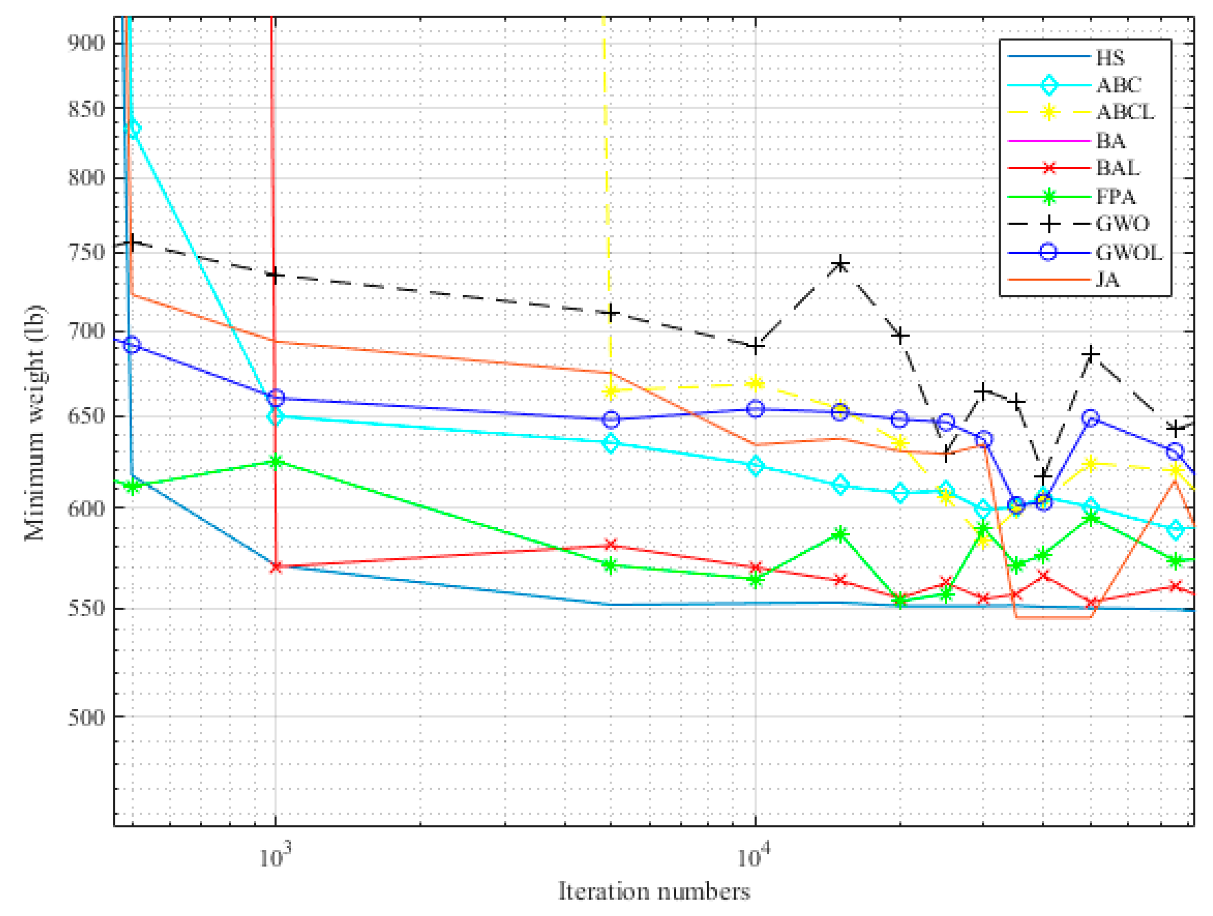
4.2. 72-Bar Truss Optimization with Bar Grouping

According to Figure 7, with the usage of a constant population with various iterations, it can be said that the most effective methods are FPA and JA cause that the other ones could not make convergence exactly to the minimum structural weight of the 72 bar truss structure. However, the best one is JA by reaching the minimum weight of 379.617 lb. In addition, in this case, Lèvy flight is notably efficient for only GWO.
On the other respect, via Table 9 and Table 10, it is seen that the best algorithm is JA in finding the minimum weight as 379.6156 lb by deviating from this value with a so small rate. Although the provided result by JA is close to the best ones among literature studies in general scope, this can be considered as a more effective method thanks to the small deviation.
Moreover, the other algorithms are not successful in an exact way in terms of reaching the minimum weight value besides that FPA has a comparatively efficient performance. However, positive effects (such as decreasing of standard deviation, etc.) and performance of Lèvy flight on the benefited algorithms are drawn attention in the direction of the realization of the optimization target. In this case, the Lèvy flight function improved, especially GWO, by decreasing weight by nearly 13 lb amount.

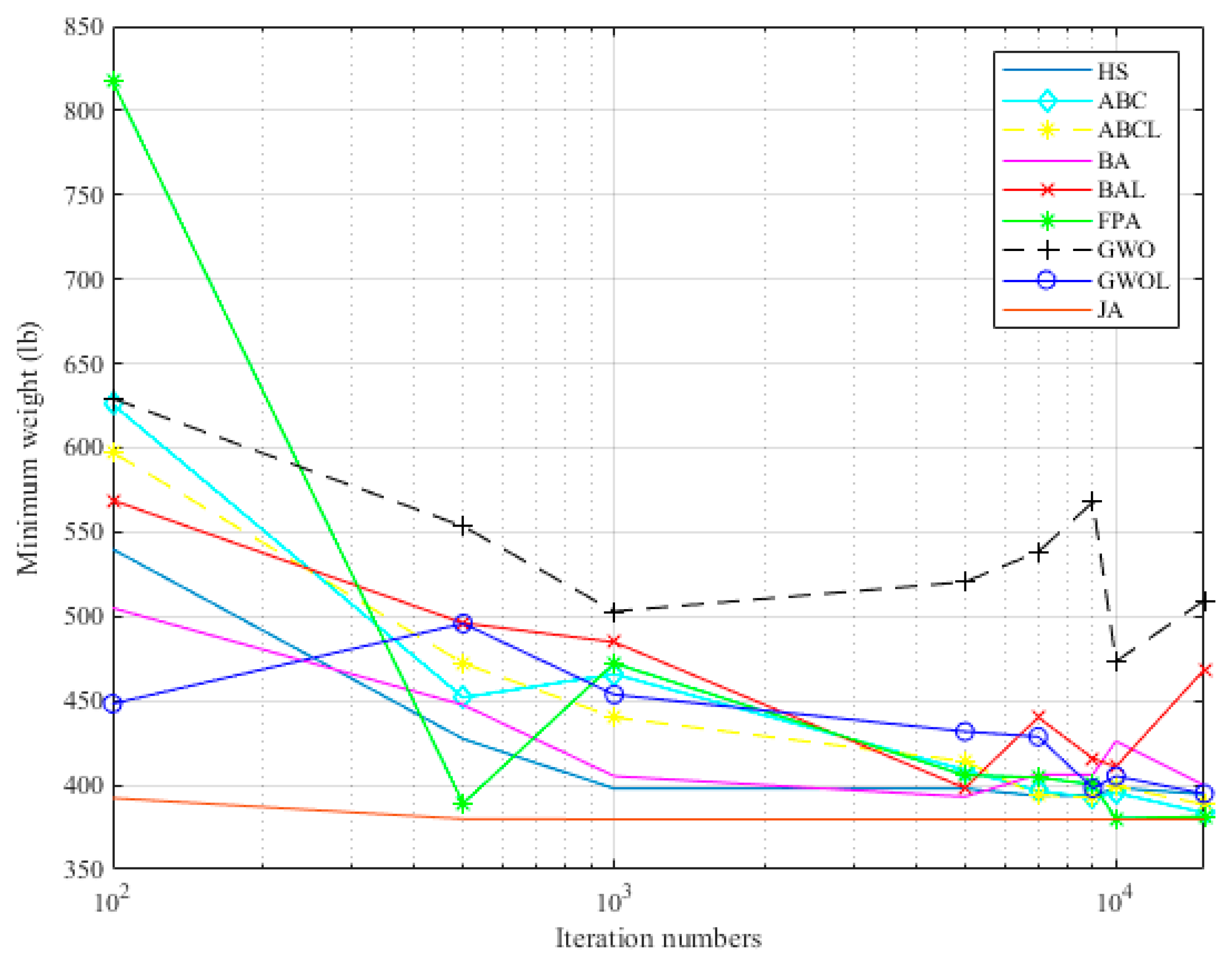
4.3. 25-Bar Truss Optimization without Bar Grouping

It can be understood from Figure 8; the best method is only JA through the achievement of the minimized truss weight as 545.108 lb for 25 bar without grouping of bars. HS, FPA, and BAL also can be accepted as usable relatively to the other ones. Furthermore, Lèvy flight affected all handled algorithms positively in the sense of convergence to more the minimized weight.
According to Table 11, JA is the top-ranking between the expressed all techniques (literature and current studies) by far thanks to minimizing of truss weight as 542.9822 lb; even this result was got via the pretty minor rate for deviation as 8.22 × 10⁻³. On the other side, Lèvy flight influenced all population-based algorithms utilizing reduction of minimum weight with comparison to the classical structure of the mentioned methods. Additionally, this function provides to decrease of the best necessary iteration numbers for ABC with GWO, too.

5. Conclusions

As a result, it can be said that the JA algorithm is the best option to be benefitted from the minimization of the structural weight regarded the handled truss models. This algorithm could succeed in this operation by providing to occur of very small standard deviations, too. On the other side, when the Lèvy flight was evaluated, the constant population taken as 30 is always not good to prefer in terms of improving minimization performance for swarm intelligence-based algorithms according to both cases compared to each other. Because it can be understood from the results, algorithms combined with Lèvy flight are more powerful and efficient about finding the optimum value of the weight when the population number shows a change by adjusting the required iteration numbers.
Except for these, Lèvy flight is chiefly useful for developing of GWO algorithm’s minimization performance compared with the other ones. For this respect, in the other optimization studies, hybridization of GWO with this function can be benefited for many objectives.

Author Contributions

Conceptualization, G.B., M.Y. and S.M.N.; methodology, G.B., M.Y. and S.M.N.; software, G.B. and M.Y.; validation, M.Y. and S.M.N.; formal analysis, G.B., M.Y. and S.M.N.; investigation, M.Y.; resources, M.Y.; data curation, M.Y.; writing—original draft preparation, M.Y.; writing—review and editing, S.M.N.; visualization, M.Y.; supervision, G.B and S.M.N.; project administration, G.B. All authors have read and agreed to the published version of the manuscript.

Funding

This study was funded by the Scientific Research Projects Coordination Unit of Istanbul University-Cerrahpaşa. Project number: FYO-2019-32735.

Data Availability Statement

The corresponding data of the paper can be obtained by requesting via e-mail to the corresponding author.

Conflicts of Interest

The authors declare no conflict of interest.

Appendix A

Table A1. Some expressions used as special by BA.
AbbreviationExplanation
V i , n e w New velocity value for ith design variable
V i , j Current velocity value of ith design variable within jth candidate solution (bat)
f j Frequency of jth candidate solution
A m e a n Mean of sound loudness values belonging all bats
A j , n e w New value, which will be assigned for loudness for ith bat
r j , n e w New value, which will be determined for sound vibration emission rate of bats
Table A2. Indication of basic and special algorithm parameters.
NotationPropertyAlgorithm
Population NumberHMSTotal harmony number or harmony memory sizeHS
e b / o b / f s n Number of employee bee/onlooker bee/food source numberABC
f n Number of total firefliesFA
b n Number of batsBA
n f Total flower numberFPA
w n Gray wolf number in the packGWO
p n Population numberJA
Characteristic ParametersPARParameter providing of generating random number depended on music tone, between limits of variable/pitch adjusting rateHS
HMCRHarmony memory consideration rate
ip Parameter, which takes value according to the case that food sources can be optimizedABC
SILLimit condition, which is considered for which sources must be renewed by scout bees and is assigned at the beginning of the optimization
β 0 Minimum ( r jk = 0 ) attractiveness value ( β 0 [ 0 , 1 ] )FA
γLight absorption coefficient ( γ [ 0 , 1 ] )
α t Randomization parameter
f min Minimum value of frequencyBA
f max Maximum value of frequency
A 0 Loudness of bats during the initial state
A min Minimum value of sound loudness
r j 0 Sound vibration emission rate of bats in the initial state
βRandom number, which is determined in the range [−1,1]
αConstant coefficient that effective for transmission of loudness
γConstant coefficient that determines of sound vibration emission rate
sp Switch probability/search changeFPA
C Coefficient vectorGWO
A Vector determining the case that wolf attacks to prey
a Vector affecting the distance between prey with wolf
Table A3. Definition of expressions used in algorithms as general and commonly.
ExpressionExplanationAlgorithm
Some Solution Values
for
Design
Variables
X i , new New value of ith design variableAll
X i , min Low limit of ith design variable (minimum value)HS
ABC
X i , max Upper limit of ith design variable (maximum value)
X i , j Initial matrix value of jth candidate solution belonging to ith design variableAll out of HS
X i , g best ith design variable value belongs to the solution with the best value in terms of the objective functionAll out of HS, ABC, and FA
X i , g worst ith design variable value belongs to the solution with the worst value in terms of the objective functionJA
X i , n Value of nth solution for ith design variableFPA
HS
X i , m Value of mth solution for ith design variableFPA
X i , k Value of a specific kth firefly for ith design variableFA
X i , pr Initial matrix value of ith design variable corresponding to pth solution (prey)GWO
X p ,   new New value of pth design variableABC
X p , j Value (in initial solution matrix) of jth solution for pth design variable
X p , n nth solution value of pth design variable
Optimization Elements n nth candidate vector selected randomly from the initial matrixAll out of BA, FA, and JA
M mth candidate vector selected randomly from the initial matrixFPA
P Randomly selected parameter as from whole design variablesABC
vnNumber of total design variable, which will be optimizedFA, ABC
TStage of the current iterationFA, BA, GWO
stopping criteriaTotal iteration numberGWO
Table A4. Functions utilized in algorithms.
NameTaskAlgorithm
FunctionsrandGeneration random number between 0 and 1All
ceil ( )Round the number in parentheses to equal/bigger natural number than itFPA, ABC, HS
min ( )Determine the smallest one among value in a certain amountAll out of HS and ABC
max ( )Determine the biggest one among value in a certain amountJA
mean ( )Calculate the average of element values in an arrayBA
abs ( )Absolute of number within the parenthesesJA, GWO
sort ( )Queue the members in any array from small to bigGWO
exp ( )Give the power of e to the degree of number within parenthesesFPA
sqrt ( )Take the square root of a numberFA
sum ( )Give the total of element values in any number arrayABC

References

  1. Bekdaş, G.; Nigdeli, S.M. Mass ratio factor for optimum tuned mass damper strategies. Int. J. Mech. Sci. 2013, 71, 68–84. [Google Scholar] [CrossRef]
  2. Parcianello, E.; Chisari, C.; Amadio, C. Optimal design of nonlinear viscous dampers for frame structures. Soil Dyn. Earthq. Eng. 2017, 100, 257–260. [Google Scholar] [CrossRef]
  3. Talatahari, S.; Gandomi, A.H.; Yang, X.S.; Deb, S. Optimum design of frame structures using the eagle strategy with differential evolution. Eng. Struct. 2015, 91, 16–25. [Google Scholar] [CrossRef]
  4. Gholizadeh, S.; Ebadijalal, M. Performance based discrete topology optimization of steel braced frames by a new metaheuristic. Adv. Eng. Softw. 2018, 123, 77–92. [Google Scholar] [CrossRef]
  5. Fathali, M.A.; Rohollah, S.; Vaez, H. Optimum performance-based design of eccentrically braced frames. Eng. Struct. 2020, 202, 109857. [Google Scholar] [CrossRef]
  6. Kayabekir, A.E.; Bekdaş, G.; Nigdeli, S.M. Metaheuristic Approaches for Optimum Design of Reinforced Concrete Structures: Emerging Research and Opportunities; IGI Global: Hershey, PA, USA, 2020. [Google Scholar]
  7. Vaez, S.R.H.; Qomi, H.S. Bar layout and weight optimization of special RC shear wall. Structures 2018, 14, 153–163. [Google Scholar] [CrossRef]
  8. Sheikholeslami, R.; Khalili, B.G.; Sadollah, A.; Kim, J. Optimization of reinforced concrete retaining walls via hybrid firefly algorithm with upper bound strategy. KSCE J. Civ. Eng. 2016, 20, 2428–2438. [Google Scholar] [CrossRef]
  9. Aydogdu, I. Cost optimization of reinforced concrete cantilever retaining walls under seismic loading using a biogeography-based optimization algorithm with Lèvy flights. Eng. Optim. 2017, 49, 381–400. [Google Scholar] [CrossRef]
  10. Camp, C.V. Design of space trusses using Big Bang–Big Crunch optimization. J. Struct. Eng. 2007, 133, 999–1008. [Google Scholar] [CrossRef]
  11. Gomes, H.M. Truss optimization with dynamic constraints using a particle swarm Algorithm. Expert Syst. Appl. 2011, 38, 957–968. [Google Scholar] [CrossRef]
  12. Miguel, L.F.F.; Miguel, L.F.F. Shape and size optimization of truss structures considering dynamic constraints through modern metaheuristic algorithms. Expert Syst. Appl. 2012, 39, 9458–9467. [Google Scholar] [CrossRef]
  13. Bekdaş, G.; Nigdeli, S.M.; Yang, X.S. Sizing optimization of truss structures using flower pollination algorithm. Appl. Soft Comput. 2015, 37, 322–331. [Google Scholar] [CrossRef]
  14. Kaveh, A.; Ghazaan, M.I. Vibrating particles system algorithm for truss optimization with multiple natural frequency constraints. Acta Mech. 2017, 228, 307–322. [Google Scholar] [CrossRef]
  15. Tejani, G.G.; Pholdee, N.; Bureerat, S.; Prayogo, D. Multiobjective adaptive symbiotic organisms search for truss optimization problems. Knowl. Based Syst. 2018, 161, 398–414. [Google Scholar] [CrossRef]
  16. Dede, T.; Bekiroğlu, S.; Ayvaz, Y. Weight minimization of trusses with genetic algorithm. Appl. Soft Comput. 2011, 11, 2565–2575. [Google Scholar] [CrossRef]
  17. Gandomi, A.H.; Alavi, A.H.; Talatahari, S. Structural Optimization Using Krill Herd Algorithm. In Swarm Intelligence and Bio-Inspired Computation; Elsevier: Amsterdam, The Netherlands, 2013; pp. 335–349. [Google Scholar]
  18. Degertekin, S.O.; Hayalioglu, M.S. Sizing truss structures using teaching-learning-based optimization. Comput. Struct. 2013, 119, 177–188. [Google Scholar] [CrossRef]
  19. Kaveh, A.; Bakhshpoori, T.; Afshari, E. An efficient hybrid particle swarm and swallow swarm optimization algorithm. Comput. Struct. 2014, 143, 40–59. [Google Scholar] [CrossRef]
  20. Kaveh, A.; Sheikholeslami, R.; Talatahari, S.; Keshvari-Ilkhichi, M. Chaotic swarming of particles: A new method for size optimization of truss structures. Adv. Eng. Softw. 2014, 67, 136–147. [Google Scholar] [CrossRef]
  21. Camp, C.V.; Farshchin, M. Design of space trusses using modified teaching–learning based optimization. Eng. Struct. 2014, 62, 87–97. [Google Scholar] [CrossRef]
  22. Bureerat, S.; Pholdee, N. Optimal truss sizing using an adaptive differential evolution algorithm. J. Comput. Civ. Eng. 2016, 30, 04015019. [Google Scholar] [CrossRef]
  23. Degertekin, S.O.; Lamberti, L.; Hayalioglu, M.S. Heat transfer search algorithm for sizing optimization of truss structures. Lat. Am. J. Solids Struct. 2017, 14, 373–397. [Google Scholar] [CrossRef]
  24. Bekdaş, G.; Nigdeli, S.M.; Yang, X.S. Size optimization of truss structures employing flower pollination algorithm without grouping structural members. Int. J. Theor. Appl. Mech. 2017, 1, 269–273. [Google Scholar]
  25. Yang, X.S. Flower pollination algorithm for global optimization. In International Conference on Unconventional Computing and Natural Computation; Springer: Berlin/Heidelberg, Germany, 2012; pp. 240–249. [Google Scholar]
  26. Yang, X.S.; Koziel, S.; Leifsson, L. Computational optimization, modelling and simulation: Recent trends and challenges. Procedia Comput. Sci. 2013, 18, 855–860. [Google Scholar] [CrossRef] [Green Version]
  27. Yang, X.S.; Bekdaş, G.; Nigdeli, S.M. (Eds.) Metaheuristics and Optimization in Civil Engineering; Springer: Cham, Switzerland, 2016; ISBN 9783319262451. [Google Scholar]
  28. Karaboga, D. An Idea Based on Honey Bee Swarm for Numerical Optimization; Technical Report-tr06; Computer Engineering Department, Engineering Faculty, Erciyes University: Talas, Turkey, 2005; Volume 200, pp. 1–10. [Google Scholar]
  29. Erdoğmuş, P. Doğadan esinlenen optimizasyon algoritmaları ve optimizasyon algoritmalarının optimizasyonu. Düzce Üniversitesi Bilim Ve Teknol. Derg. 2016, 4, 293–304. [Google Scholar]
  30. Tapao, A.; Cheerarot, R. Optimal parameters and performance of artificial bee colony algorithm for minimum cost design of reinforced concrete frames. Eng. Struct. 2017, 151, 802–820. [Google Scholar] [CrossRef]
  31. Yahya, M.; Saka, M.P. Construction site layout planning using multi-objective artificial bee colony algorithm with Lèvy flights. Autom. Constr. 2014, 38, 14–29. [Google Scholar] [CrossRef]
  32. Karaboga, D.; Basturk, B. A powerful and efficient algorithm for numerical function optimization: Artificial bee colony (ABC) algorithm. J. Glob. Optim. 2007, 39, 459–471. [Google Scholar] [CrossRef]
  33. Yang, X.S. A New Metaheuristic Bat-Inspired Algorithm; Nature Inspired Cooperative Strategies for Optimization (NICSO 2010); González, J.R., Pelta, D.A., Cruz, C., Terrazas, G., Krasnogor, N., Eds.; Springer: Berlin/Heidelberg, Germany, 2010; ISBN 9783642125386. [Google Scholar]
  34. Gandomi, A.H.; Yang, X.S.; Talatahari, S.; Alavi, A.H. (Eds.) Metaheuristic Algorithms in Modeling and Optimization. In Metaheuristic Applications in Structures and Infrastructures; Elsevier: Amsterdam, The Netherlands, 2013; pp. 1–24. [Google Scholar]
  35. Kaveh, A.; Zakian, P. Enhanced bat algorithm for optimal design of skeletal structures. Asian J. Civ. Eng. 2014, 15, 179–212. [Google Scholar]
  36. Rao, R. Jaya: A simple and new optimization algorithm for solving constrained and unconstrained optimization problems. Int. J. Ind. Eng. Comput. 2016, 7, 19–34. [Google Scholar]
  37. Mirjalili, S.; Mirjalili, S.M.; Lewis, A. Grey wolf optimizer. Adv. Eng. Softw. 2014, 69, 46–61. [Google Scholar] [CrossRef] [Green Version]
  38. Doğan, C. Balina Optimizasyon Algoritması ve gri Kurt Optimizasyonu Algoritmaları Kullanılarak yeni Hibrit Optimizasyon Algoritmalarının Geliştirilmesi. Master’s Thesis, T.C. Erciyes University, Kayseri, Turkey, 2019. [Google Scholar]
  39. Doğan, L. Robot yol Planlaması için gri kurt Optimizasyon Algoritması. Master’s Thesis, Bilecik Şeyh Edebali University, Bilecik, Turkey, 2018. [Google Scholar]
  40. Faris, H.; Aljarah, I.; Al-Betar, M.A.; Mirjalili, S. Grey wolf optimizer: A review of recent variants and applications. Neural Comput. Appl. 2018, 30, 413–435. [Google Scholar] [CrossRef]
  41. Şahin, İ.; Dörterler, M.; Gökçe, H. Optimum design of compression spring according to minimum volume using grey wolf optimization method. Gazi J. Eng. Sci. 2017, 3, 21–27. [Google Scholar]
  42. Geem, Z.W.; Kim, J.H.; Loganathan, G.V. A new heuristic optimization algorithm: Harmony search. Simulation 2001, 76, 60–68. [Google Scholar] [CrossRef]
  43. Bekdaş, G.; Nigdeli, S.M. Değişik periyotlu yapılar için optimum pasif kütle sönümleyici özelliklerinin belirlenmesi. In 1. Türkiye Deprem Mühendisliği ve Sismoloji Konferansı; 11–14 Ekim; ODTÜ: Ankara, Turkey, 2011; pp. 1–8. [Google Scholar]
  44. Koziel, S.; Yang, X.S. (Eds.) Computational Optimization, Methods and Algorithms; Springer: Berlin/Heidelberg, Germany, 2011; Volume 356, ISBN 978-3-642-20858-4. [Google Scholar]
  45. Rao, S.S. Engineering Optimization Theory and Practice, 4th ed.; John Wiley & Sons: Hoboken, NJ, USA, 2009; ISBN 978-0-470-18352-6. [Google Scholar]
Figure 1. Social hierarchy pyramid among gray wolves [39].
Buildings 11 00049 g001
Figure 2. Determining the new position of any omega wolf concerning prey according to wolves α, β, and δ [40].
Buildings 11 00049 g002
Figure 3. Condition of attack to prey by omega (ω) wolf, and the possible cases of its new position determined according to prey [41].
Buildings 11 00049 g003
Figure 4. Design model and variables of a 25 bar truss structure [13].
Buildings 11 00049 g004
Figure 5. Design model and variables of a 72 bar truss structure [13].
Buildings 11 00049 g005
Figure 6. Variation of the values for minimum weight corresponding to different iteration numbers with a constant (30) population.
Buildings 11 00049 g006
Figure 7. Minimum weight changing ensured according to multiple iteration numbers and a constant (30) population.
Buildings 11 00049 g007
Figure 8. Changing for minimum weight values concerning different iteration numbers via a constant (30) population.
Buildings 11 00049 g008
Table 1. Comparing some literature research and the present study.
ResearchersNumber of
Used Classical Algorithms
Number of Hybridized/
Modified Algorithms
AlgorithmNumber of Investigated Truss ModelsNumber of Maximum Design VariablesBiggest Number of Compared Other MethodsCitation
Camp (2007)1-Big bang–big crunch (BB–BC) optimization3164[10]
Dede et al. (2011)1-Genetic algorithm (GA)49613[16]
Gandomi et al. (2013)1-Krill herd (KH)1810[17]
Degertekin and Hayalioglu (2013)1-Teaching-learning based optimization (TLBO)4298[18]
Kaveh et al. (2014)-1Hybrid particle swarm and swallow swarm optimization (HPSSO)6296[19]
Kaveh et al. (2014b)-1Chaotic swarming of particles (CSP)4595[20]
Camp and
Farschin (2014)
-1Modified teaching-learning based optimization (TLBO)3267[21]
Bureerat and Pholde (2016)-1Adaptive
Differential evolution algorithm (ADEA)
4296[22]
Degertekin et al. (2017)1-Heat transfer search (HTS)3298[23]
Bekdaş et al. (2017)1-Flower pollination algorithm (FPA)2720[24]
Present Study63Defined in Section 23257-
Table 2. Information for optimization process corresponding for 25 and 72 bar truss structures.
DefinitionSymbolLimit/ValueUnitTruss Model
Design
Variables
Cross-section of truss barsAbar0.01–3.4
0.1–3.0
inch225-Bar
72-Bar
Design
Constants
Elasticity modulusEs107psiBoth
Weight per unit of volume of barsρs0.1lb/inch3
Bar number-25
72
-25-Bar
72-Bar
Node number-10
20
-25-Bar
72-Bar
Bar group number-8
16
-25-Bar
72-Bar
Table 3. Loading conditions on nodes for a 25 bar truss model.
CaseNode
Number
LoadUnit
PxPyPz
11100010,000−5000lb/inch2
2010,000−5000
350000
650000
21020,000−5000
20−20,000−5000
Table 4. Loading conditions on nodes for a 72 bar truss model.
CaseNode
Number
LoadUnit
PxPyPz
11750005000−5000lb/inch2
21700−5000
1800−5000
1900−5000
2000−5000
Table 5. The design constraints for a 25 bar truss structure.
Structural MemberDescriptionConstraintsUnit
NodesDisplacement
AllLimitation of Displacements Occurred on Nodes δ < | 0.35 | inch
Group
Number
Design
Variables
Compression
Stress
Tension
Stress
1A1Limitation required for stresses occurred on bars σ c > 35 , 092 σ t < + 40 , 000 psi
2A2–5 σ c > 11 , 590
3A6–9 σ c > 17 , 305
4A10–11 σ c > 35 , 092
5A12–13 σ c > 35 , 092
6A14–17 σ c > 6759
7A18–21 σ c > 6959
8A22–25 σ c > 11 , 080
Table 6. The design constraints for a 72 bar truss structure.
Structural MemberDescriptionConstraintsUnit
NodesDisplacement
AllLimitation of Displacements Occurred on Nodes δ < | 0.25 | inch
Group
Number
Design
Variables
Compression
Stress
Tension
Stress
1A1–4Limitation required for stresses occurred on bars σ c > 25 , 000 σ t < + 25 , 000 psi
2A5–12
3A13–16
4A17–18
5A19–22
6A23–30
7A31–34
8A35–36
9A37–40
10A41–48
11A49–52
12A53–54
13A55–58
14A59–66
15A67–70
16A71–72
Table 7. Optimum results ensured from previous studies for 25 bar truss with grouping.
Group NumberDesign VariablesPrevious Studies
KH [17]TLBO [18]HPSSO [19]CSP [20]TLBO [21]ADEA [22]HTS [23]
1A10.010250.01000.01000.0100.01000.01000.010000
2A2–52.024372.07121.99071.9101.98785.64062.070200
3A6–93.041542.95702.98812.7982.99148.59412.970031
4A10–110.010290.01000.01000.0100.01020.01000.010000
5A12–130.010810.01000.01000.0100.01000.01000.010000
6A14–170.689500.68910.68240.7080.68281.93680.670790
7A18–211.620021.62091.67641.8361.67754.78571.617120
8A22–252.655012.67682.66562.6452.66407.59212.698100
Best weight545.175545.09545.164545.09545.175545.1657545.13
Mean weight545.483545.41545.556545.20545.483545.2200545.47
Standard deviation0.3060.420.4320.4870.3060.07300.476
Population number-30-50---
Iteration number---350---
Total analysis number12,19915,31813,32617,50012,19910,0007653
HTS: heat transfer search, ADEA: adaptive differential evolution algorithm, HPSSO: hybrid particle swallow swarm optimization, CSP: chaotic swarming of particles, TLBO: teaching-learning based optimization, KH: krill herd.
Table 8. Optimization results and the best parameters for 25 bar truss with bar grouping.
Group NumberDesign VariablesCurrent Study
HSABCABCLBABALFPAGWOGWOLJA
1A10.01000.01150.01000.01000.01000.01000.02290.01080.0100
2A2–52.13751.91932.10711.96941.97742.04911.92292.00442.0420
3A6–92.89103.15492.93463.13563.05073.03413.07123.04223.0045
4A10–110.01000.01000.01000.01000.01000.01010.01000.01040.0100
5A12–130.01000.01020.01030.01000.01020.01000.22850.01420.0100
6A14–170.68870.67490.64150.68080.69230.67700.61420.68170.6816
7A18–211.59941.66271.60511.62581.65661.60351.70701.63751.6229
8A22–252.69912.63522.75082.64322.64122.67642.72412.66072.6737
Best weight545.3419545.4145545.3736545.3712545.1191545.0738548.9530545.1282545.0378
Mean weight548.3861545.5653545.4441549.9517546.4605545.0738548.9533545.1287545.0440
Standard deviation1.1600.1040.1081.9405.5602.10 × 10−136.36 × 10−51.88 × 10−43.03 × 10⁻³
Best population
number
302530252025202020
Best iteration number18,00013,000500012,50010,000250011,00011,50015,000
Table 9. Current optimum results with the best parameters for 72 bar truss (grouping).
Group NumberDesign VariablesCurrent Study
HSABCABCLBABALFPAGWOGWOLJA
1A1–42.23012.07811.79101.76822.06791.90571.78452.04581.8899
2A5–120.49460.51870.51950.57200.48540.49160.52490.48640.5119
3A13–160.10000.10260.10000.10000.10000.10000.10000.11370.1000
4A17–180.12120.10000.10000.13840.10000.10030.10000.10030.1000
5A19–221.19851.25941.34841.35351.34571.33721.01101.11401.2702
6A23–300.50090.45590.48600.53470.53190.49070.64690.55040.5120
7A31–340.10000.10010.10000.10000.11810.10000.10000.11610.1000
8A35–360.10000.10000.10230.10000.10030.10000.10000.10630.1000
9A37–400.54770.62390.50610.61660.48390.55900.64090.51980.5234
10A41–480.53340.47100.50020.49210.51940.50880.53180.46720.5165
11A49–520.10320.10000.10000.10000.10050.10000.10000.16830.1000
12A53–540.10000.10000.10000.15670.14200.10000.35520.10000.1000
13A55–580.16260.15700.15580.16440.15620.15600.15020.15160.1565
14A59–660.50400.62020.56340.50310.52140.53730.46660.56510.5457
15A67–700.38310.38980.50240.36990.39720.48900.28460.38320.4104
16A71–720.73330.57250.57380.61290.52350.58020.96650.72470.5678
Best weight386.2662383.4078381.5569385.6475381.9249380.4598398.7166386.5409379.6156
Mean weight405.3741402.1776395.4222417.7893382.0331380.4598398.7167386.5411379.6172
Standard deviation5.82016.1008.71048.7000.2202.79 × 10−135.77 × 1053.65 × 1057.49 × 104
Best Population number253030151025153030
Best iteration number13,00014,50019,00020,00017,50018,000850019,50017,500
Table 10. Some literature studies concerning 72 bar truss (grouping).
Group NumberDesign VariablesPrevious Studies
BB-BC [10]GA [16]TLBO [18]CSP [20]TLBO [21]ADEA [22]HTS [23]
1A1–41.85771.7021.906401.944591.88071.88611.9001
2A5–120.50590.4960.506120.502600.51420.52310.5131
3A13–160.10000.1000.100000.100000.10000.10000.1000
4A17–180.10000.1000.100000.100000.10000.10000.1000
5A19–221.24761.2881.261701.267571.27111.25761.2456
6A23–300.52690.4690.511100.509900.51510.50430.5080
7A31–340.10000.1000.100000.100000.10000.10000.1000
8A35–360.10120.1000.100000.100000.10000.10000.1000
9A37–400.52090.5050.531700.506740.53170.52000.5550
10A41–480.51720.5500.515910.516510.51340.52350.5227
11A49–520.10040.1090.100000.107520.10000.10000.1000
12A53–540.10050.1180.100000.100000.10000.10000.1000
13A55–580.15650.1540.156200.156180.15650.15680.1566
14A59–660.55070.6040.549270.540220.54290.53940.5407
15A67–700.39220.4420.409660.422290.40810.40830.4084
16A71–720.59220.6040.569760.579410.57330.57340.5669
Best weight379.85379.63379.63379.97379.632379.6943379.73
Mean weight382.08--381.56379.759379.8961382.26
Standard deviation1.912--1.8030.1490.07911.940
Population number-------
Iteration number-------
Total analysis number694219,70919,70910,50021,54215,60013,166
HTS: heat transfer search, ADEA: adaptive differential evolution algorithm, CSP: chaotic swarming of particles, GA: genetic algorithm, TLBO: teaching-learning based optimization, BB-BC: big-bang big crunch.
Table 11. Optimum results provided with the best parameters for 25 bar truss without grouping.
Design
Variables
Documented Study [24]Current Study
FPAHSABCABCLBABALFPAGWOGWOLJA
A10.01000.44580.12980.01040.11840.01000.09650.77960.01030.0100
A22.39033.14942.21843.40002.01742.65151.48021.22541.95481.9019
A31.85242.04111.94491.40152.27801.69652.91222.27861.29002.4622
A42.09352.15862.03513.33511.83492.51791.21672.88932.53391.6803
A51.97492.11751.91370.73742.42921.53762.95521.65502.52932.4353
A62.95492.76722.43823.40002.83193.34452.31742.55742.88532.7733
A72.93792.79202.77382.95103.05743.25732.66652.73722.62042.7611
A83.00852.86343.09202.43973.15062.88953.24963.03882.78393.4000
A92.49742.86151.97812.31342.91352.10743.26802.97892.07612.8591
A100.01000.13320.12100.28100.12780.10410.01000.65680.01590.0100
A110.01041.61320.30370.01000.08600.02940.01000.47570.07560.0100
A120.01000.42090.01570.01960.01000.01070.11000.84140.01150.0100
A130.01000.31240.36100.01000.01000.01320.01000.34160.01540.0100
A140.70581.27631.32850.55960.78480.59930.86700.93440.91420.8295
A150.59500.46790.32220.63890.76870.62650.72450.86620.48070.6832
A160.80431.54771.11220.82790.64980.72420.64771.63821.36340.6205
A170.61490.19540.60270.59910.61660.73400.45330.49810.57720.5581
A181.70111.76481.82172.66331.62281.74181.27802.18022.44271.4748
A191.72591.02802.09101.29551.85061.70041.82262.21222.24631.8439
A201.83752.16912.13502.46771.46791.79271.47162.06112.03301.5456
A211.37931.54541.76260.82971.40961.31352.01452.08262.27091.4880
A222.34462.06153.04362.25672.35692.10483.15223.01291.73812.9342
A232.57442.05533.09272.18763.05322.62143.20853.02492.60663.0578
A243.14643.36493.00283.40003.07713.26522.56991.75453.08292.6271
A252.59202.92542.01493.40002.10052.74271.83361.90412.71112.0332
Best weight543.20585.9394573.9692565.9572549.4372545.2959548.1256604.4136578.7288542.9822
Mean weight-603.0324599.9786566.0596551.1452552.0253548.1256604.4137578.7288543.0017
Standard
deviation
-16.40017.4000.1651.18034.4001.18 × 10139.04 × 1061.79 × 10−68.22 × 10⁻³
Best population number20153015253025103015
Best iteration number100,00095,000115,00035,00030,000110,00055,000120,00090,000115,000
Publisher’s Note: MDPI stays neutral with regard to jurisdictional claims in published maps and institutional affiliations.

