Article

Spatial Analysis, Interactive Visualisation and GIS-Based Dashboard for Monitoring Spatio-Temporal Changes of Hotspots of Bushfires over 100 Years in New South Wales, Australia

1
City Analytics, University of New South Wales, Sydney, NSW 2052, Australia
2
Urban Science, University of New South Wales, Sydney, NSW 2052, Australia
*
Author to whom correspondence should be addressed.
Buildings 2021, 11(2), 37; https://doi.org/10.3390/buildings11020037
Submission received: 20 November 2020 / Revised: 17 January 2021 / Accepted: 20 January 2021 / Published: 23 January 2021

Abstract

:
The 2019–2020 bushfire season is estimated to be one of the worst fire seasons on record in Australia, especially in New South Wales (NSW). The devastating fire season ignited a heated public debate on whether prescribed burning is an effective tool for preventing bushfires, and how the extent of bushfires has been changing over time. The objective of this study is to answer these questions, and more specifically to identify how bushfire patterns have changed in the last 100 years in NSW. To do so, we conducted a spatio-temporal analysis on prescribed burns and bushfires using a 100-year dataset of bushfires. More specifically, three research questions were developed, with each one of them addressed differently. First, generalised linear modelling was applied to assess the changes in fire patterns. Second, a correlation analysis was conducted to examine whether prescribed burns are an effective tool for reducing bushfire risk. Third, a spatio-temporal analysis was applied to the bushfire location data to explore spatio-temporal clusters of high and low values for bushfires, known as hotspots and coldspots, respectively. The study found that the frequency of bushfires has increased over time; however, it did not identify a significant trend of change in their size. Based on the results of this study for the relationship between prescribed burns and bushfires, it seems impossible to determine whether prescribed burns effectively reduce bushfire risk. Thus, further analysis with a larger amount of data is required in the future. The results of the spatio-temporal analysis showed that cold spots are propagated around metropolitan areas such as Sydney, while hotspots are concentrated in rural areas such as the North Coast and South Coast regions of NSW. The analysis found four statistical areas that have become new bushfire frequency hotspots in the 2019–2020 bushfire season. These areas combined have about 40,000 residents and at least 13,000 built dwellings. We suggest that further analysis is needed in the field to determine if there is a pattern of movement of bushfire towards metropolitan areas. To make the results of this research accessible to the public, an online interactive GIS-based dashboard was developed. The insight gained from the spatial and temporal analyses in this research is crucial to making smarter decisions on allocating resources and developing preventive or mitigating strategies.

1. Introduction

In 1770, one of the most influential British explorers, Captain James Cook, sailed the Endeavour to discover a new land that he described in his journal as “The Continent of Smoke,” since the crew of the Main (the name of the ship) “saw smokes by day and fires by night upon the Main…” [1]. Approximately 250 years later, Cook’s “Continent of Smoke,” today modern Australia, is known to be one of the most fire-prone countries in the world, with a unique biota that is adapted to a reoccurring fire pattern [2,3,4]. The reason is its unique climate, which includes extreme high temperatures, low humidity and strong winds, which combine to create ideal conditions for severe fire storms [1,5,6,7]. At least once a decade, Australia faces massive, destructive bushfire events, such as the 1974–1975 and 1993–1994 fires, 2009 Black Saturday, etc. [1,5].
With a death toll of over 20 people, the recent 2019–2020 bushfire season is estimated to be one of the worst fire seasons in Australia on record [8]. Various Australian fire services estimate that these megafires burnt approximately 19 million hectares as of the 14 January 2020, and killed over one billion mammals, birds and reptiles, with a possibility that entire species have become extinct [8]. Increasing global temperatures and climate change have a significant impact on Australia’s bushfires, since intense heat, longer heat waves and longer droughts are predicted to increase the annual average fire danger in Australia by up to 30% by 2050 [6,9,10]. In fact, numerous studies on future fire activity have concluded that the frequency of weather conditions conducive to fire in southeast Australia is increasing, including in New South Wales, where a significant proportion of Australia’s population resides [6,9,10,11,12].
As Australia battled through the 2019–2020 bushfires, a public debate formed about the effectiveness of “prescribed burns” as a tool to reduce fires, i.e., deliberately starting fires in a controlled environment to clear out flammable material and forest fuels [13,14]. Using fire as a tool for forest management dates back before the European settlement in the 18th century [15,16]. In fact, fire was first used in Australia as method for hunting by Indigenous Australians [15,16], then by farmers as a way to clear bush, burn off old grass and reduce fire hazards on their farms, and most recently as a method of forest control [14]. The practice of “prescribed burning,” also known as “hazard reduction burning” or “controlled burning,” was first introduced in Australia in the 20th century by forest managers in southwestern Australia, who were trying to protect native forests from bushfires that had destructive impacts on their forests [14]. The methodology of prescribed burning is used worldwide. It is based on the theory that excluding fires from forest areas is a “recipe” for catastrophic fires, since it allows fuels to build up in the forest, and once ignited, they will lead to an extreme fire event. In accordance, the principal of prescribed burning is to ignite small-scale controlled fires in a fire-prone landscape during cool weather to reduce the amount of surface forest fuel and shrublands [13,14]. It is important to note that the initial goal of prescribed burns is not to prevent areas from burning, but to reduce their potential fire intensity, which can then be controlled more easily by fire fighters [13,14]. Two Australian studies that have analysed historical data of fires in southwest Western Australia and Victoria have concluded that prescribed burns significantly reduced the incidence and extent of bushfires, and have the ability to suppress them [13,17]. In a similar way, a wildfire simulation study conducted in Tasmania examined the result of intentionally burning all the vegetation that can handle prescribed burning in a hypothetical scenario of unlimited resources. It concluded that theoretically, prescribed burns are extremely effective in reducing fire activity; however, in order to effectively reduce fire activity, an unrealistically large area of prescribed burning would be required, accounting for an annual area 30 percent the size of Tasmania [18].
Opponents of the prescribed burning methodology can also be found throughout the literature. A study based on 34 years of fire data and weather records in southeastern Australia concluded that the effectiveness of prescribed burns significantly varies from one region to another, and that in most regions, it is likely to have very little effect on limiting the extent of wildfires [19]. In addition, Price [20] emphasise in a similar way to Furlaud [18] that large areas are required to be burned in order to significantly reduce the risk of bushfires. Another claim is that prescribed burning in remote areas has little impact on reducing fire risk compared to prescribed burning in residential areas [20], which can be five times more effective [21]. In addition, there is evidence in the literature that prescribed burning takes a toll on both the ecosystem and public health. This includes smoke pollution [22], a decline in biodiversity [23] and even escaped prescribed burns that go out of control and become wildfires, such as in Margaret River in Western Australia in 2013. All of the above lead to the question of whether prescribed burns are, in fact, effective or not.
Predicting the likelihood and the intensity of fires has been a common practice in fire agencies around the globe for decades. In the 1960s, the McArthur Forest Fire Danger Index (FFDI), a common index for assessing bushfire hazard, was developed by CSRIO (Commonwealth Scientific and Industrial Research Organisation) scientist A.G. McArthur [24]. Another common index, used by the Rural Fire Service in NSW, is the Bushfire Prone Area index. Similar to the FFDI, it mainly uses geographical attributes to assess fire danger, but, as opposed to displaying the fire hazard at a specific time, it represents the potential areas that have a fire risk overall [25]. The common ground of these different indexes is that they were created by using a combination of geographic attributes, a process that is usually done with GIS.
Geographic information systems (GIS) are computer-assisted systems designed to capture, store, retrieve, manipulate, manage and analyse spatial data, i.e., information that is identified by a geographic location of features and boundaries [26]. Since their emergence in the mid-1980s, GIS have become an important tool for fire prediction and analysis, because they provide ecosystem mangers the ability to simulate multiple conditions across space [27]. More specifically, GIS have the ability to identify crucial requirements for forest fire management by identifying hotspots and evaluating the risk probability and measures to reduce fire risk [28]. This is why fire agencies across the world have embraced GIS as a tool to effectively handle fires, and balance the needs, uses and hazards to promote sustainability of the environment and develop response strategies for certain fire events [27]. In fact, many countries around the world are investing in the development of geographical fire information systems to improve their fire-management abilities [29]. For example, in 2004, the European commission developed the European Forest Fire Information System (EFFIS), which includes forest fire data from 14 different member states; since 2008, it has provided maps of fire danger anomalies based on its fire index [30]. Another example is Canada, which developed the Canadian National Fire Database, a collection of point and polygon data of all the fires in a size greater than 200 hectares [31]. There are numerous other examples of countries around the globe that have developed geographical information systems. While the databases differ from one country to another, they share the same principal aim of having a fire database to allow a better understanding of fire patterns, and increase the ability to predict them [29].
Adopting a GIS approach to predict fire and examine how bushfire patterns change over space and time is not new to fire studies. A study in 2002 combined different geographical factors that contribute to fire, such as topography, land cover, vegetation, etc. to create a forest fire risk model [32]. In the past few years, fire data is being developed better and becoming more publicly available. This is highly beneficial, since predicting and analysing fire patterns have become more accessible [33,34,35]. As a result, various spatial studies in the Australia—New Zealand region analysed fire prediction methods based on geographic attributes in both small and large spatial extents. Some of these studies [3,36,37] modelled the predicted probability of bushfire occurrence in different areas in Australia based on different geographic attributes such as climate, elevation and land cover; while other studies [4,38] used historical fire data to analyse fire patterns and occurrence intervals. In a similar way, Dutta [39] integrated fire data for 336 weeks to examine fire patterns in Australia, and found that the frequency of bushfires increased between 2011–2016 by 40%. On the other hand, Sewell [40] used fire occurrence data as part of a “disaster declarations” hotspot analysis that aggregated bushfire, flood and storm data.
GIS have the potential to bring together different data and information, whether static or not, and turn into insights that serve as intelligence for emergencies and catastrophic events. These insights can then be shared with other emergency agencies or can be published publicly. GIS have the ability to aggregate and visualise multiple datasets, and therefore have a great potential for responding to disasters and extreme weather events, including bushfires, while dashboards are platforms that provide key insights for at-a-glance decision-making [41].
Nevertheless, there is a gap in bushfire research in Australia. To date, the use of historical bushfire data to identify spatio-temporal patterns of bushfires based on 100 years of bushfire data in New South Wales has not been documented. A spatio-temporal data analysis has the potential to reveal unexpected fire patterns and relationships that are hidden within databases; however, none of the above studies have included a spatio-temporal analysis based on historical bushfire data to assess patterns of fires over space and time. The main objective of this study is to fill these gaps, by using more than 100 years of bushfire data in New South Wales to conduct a spatio-temporal analysis that will reveal the temporal patterns hidden in the bushfire data. The study aims to analyse these patterns to identify how the bushfire patterns have changed in the last 100 years and in comparison to the 2019–2020 bushfire season. It is important to note that it is not within the scope of this study to consider what might cause bushfire patterns to change in New South Wales and whether the causes for change are a result of man-made or natural factors such as changes in climate patterns. Another key objective of this study is to publish its results in an online GIS platform, which will allow other researchers and practitioners to have access to the processed data and corresponding results, unlike in other studies in which the data and results are buried in papers.
This study has developed three research questions that the spatio-temporal analysis aims to answer. These are aligned with some of the questions that arose during the 2019–2020 bushfire season that became a public debate:
  • Is there a change in the pattern of bushfires in NSW over time?
  • Are areas of prescribed burns negatively correlated to areas where bushfires have occurred, i.e., do prescribed burns help to reduce bushfire risk?
  • Is the frequency of bushfires spatially clustered over time? Did these clusters change over the 2019–2020 bushfire season?

2. Materials and Methods
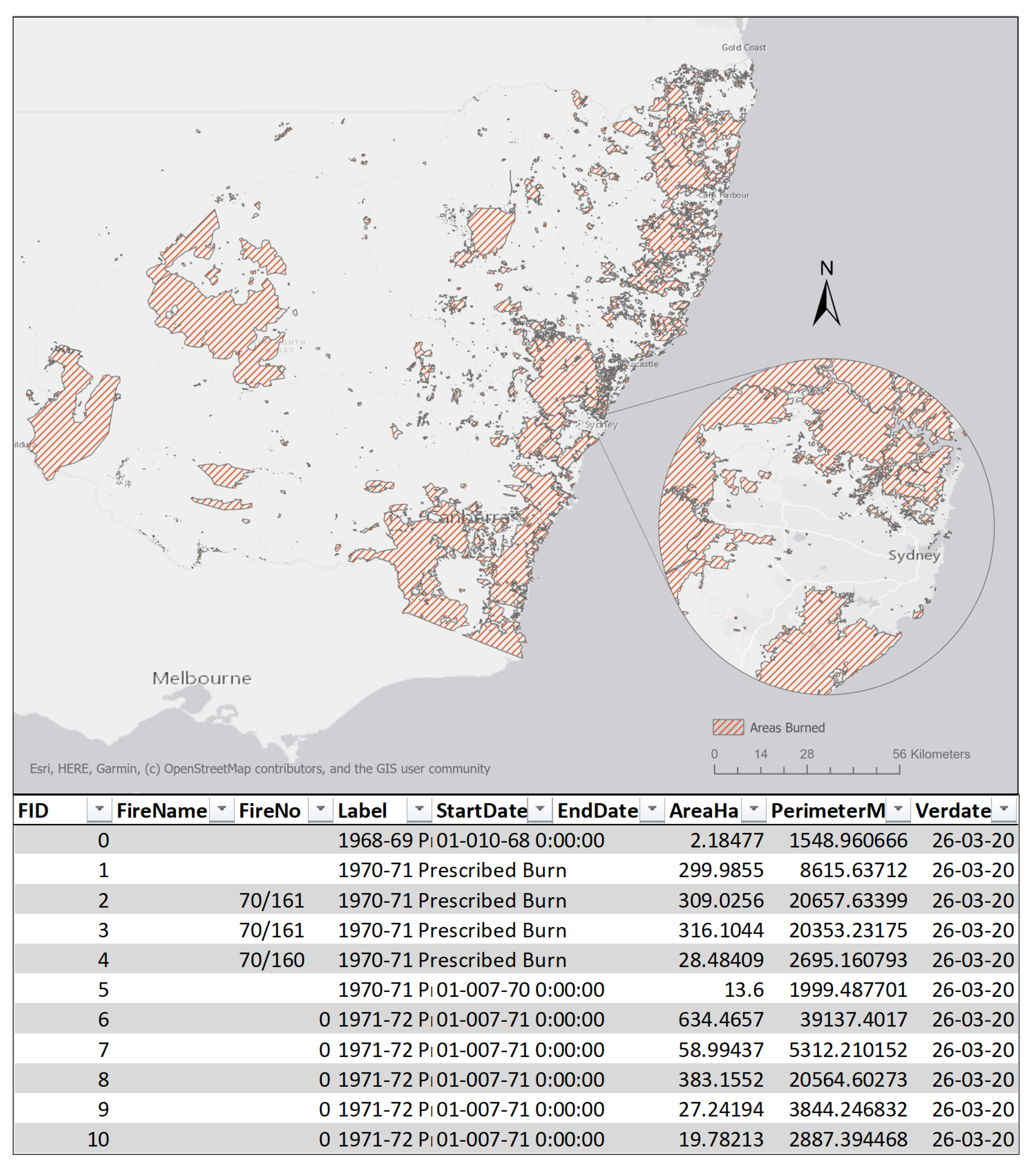
This study used a GIS approach to analyse more than 100 years of bushfire data. The data was analysed in a two-step approach by importing the data into ArcGIS/ArcGIS Pro and R databases for management and analysis, and included: (1) summarising and counting bushfire data for a statistical analysis; (2) identifying spatio-temporal patterns using hotspot analysis, emerging hotspot methods, as well as a space-time cube.

2.1. Study Area

The study area of this analysis was the State of New South Wales (NSW) in Australia. NSW is located in southeastern Australia, bounded by the Pacific Ocean and the states of Victoria and Queensland (Figure 1). The area of NSW is approximately 800 km2, meaning that it is not Australia’s largest state; however, despite its size, it is still the most populated state in the country, with nearly 7.5 million residents [42].

2.2. Data

The primary data source that stands at the base of this research is a polygon shapefile that was published by the NSW State Government and the NSW Department of Planning, Industry and Environment (2010) [43], publicly available under a Creative Commons public license. The dataset visualises the final fire boundaries for every fire in NSW since 1900 in a vector format. Each of the polygon’s attributes are described in an attribute table that contains information about each fire’s date, season, type, area and perimeter (Figure 2).

2.3. Pre-Processing of Data and Data Analysis

First, the data were imported into ArcGIS Pro to create a unique ID field in order to be able to link each polygon to its attribute if needed during the analysis. Then the data was converted into a CSV file using ArcGIS Pro and used in R (Figure 3 and Figure 4), in which three columns were added based on the “Label” column: (1) Season—describes the fire season when the fire occurred; (2) Type—classifies whether the fire is a controlled man-made fire (prescribed burn) or a bushfire (wildfire); (3) Decade—describes the decade in which the fire occurred, e.g., 1960s. Since there is not sufficient data for both prescribed burns and bushfires before 1957, the data has been filtered for further analysis to include only fires from 1957 onward.

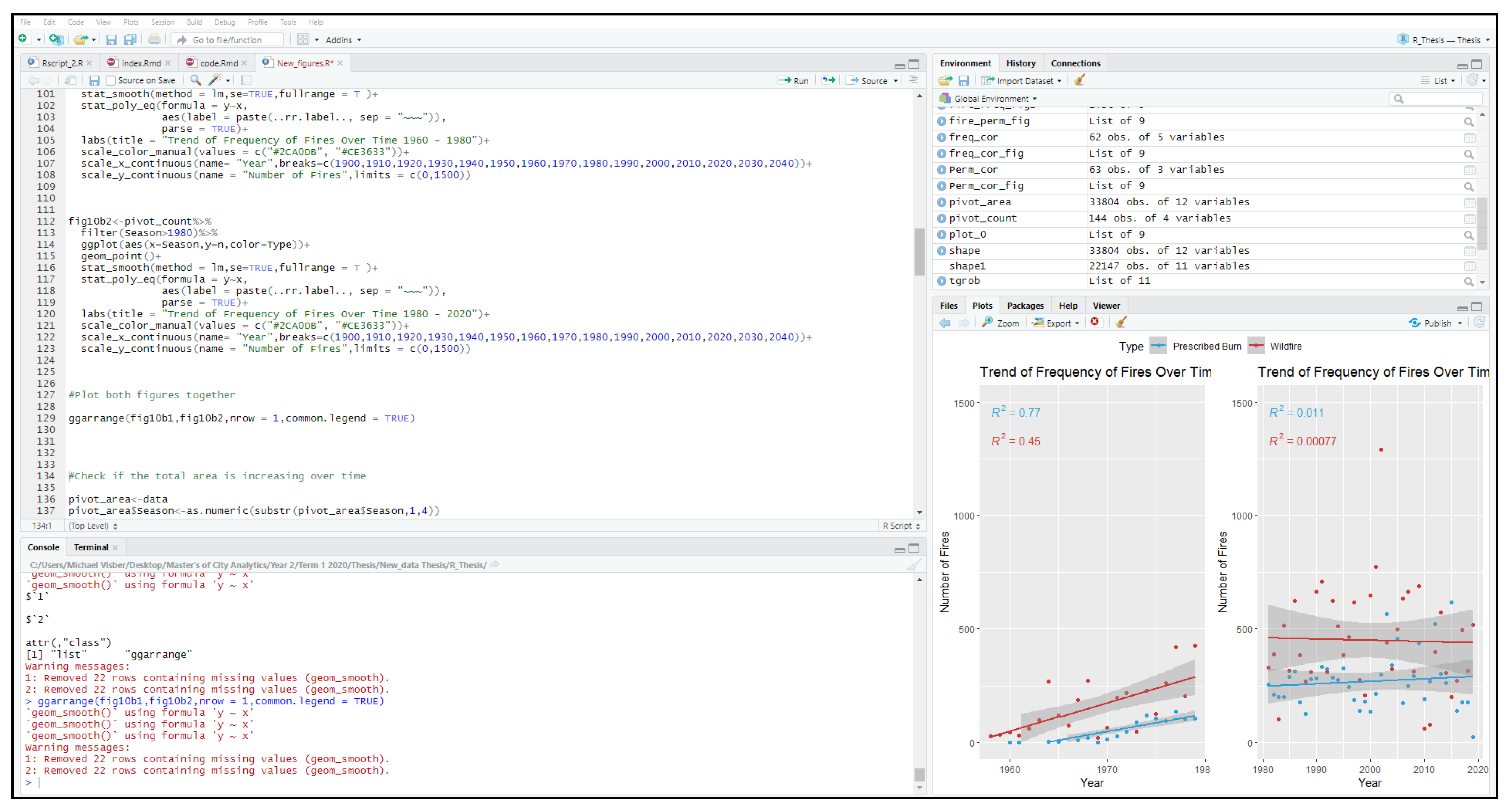
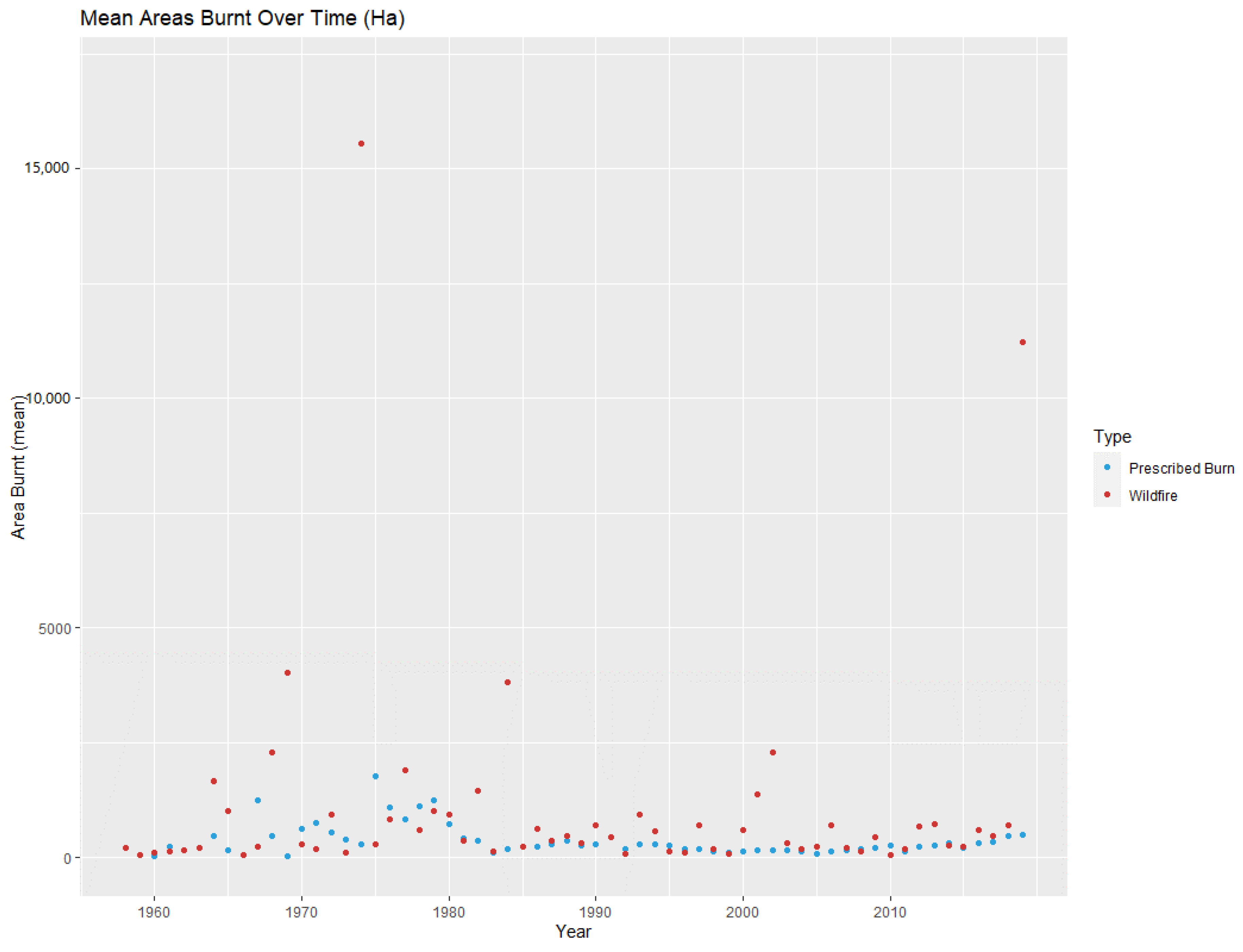
2.3.1. Change in Bushfire Trends over Time

To explore the temporal associations of the bushfire data, a generalised linear modelling method was adopted using R [36] to examine the hypothesis that the frequency of bushfires and extreme bushfire events is increasing in NSW, in a similar way to the Australian trend, as suggested by the literature [6,9,39,44]. Since the data set does not include any prescribed burns before the end of the 1950s, features prior to 1957 were removed from this analysis.

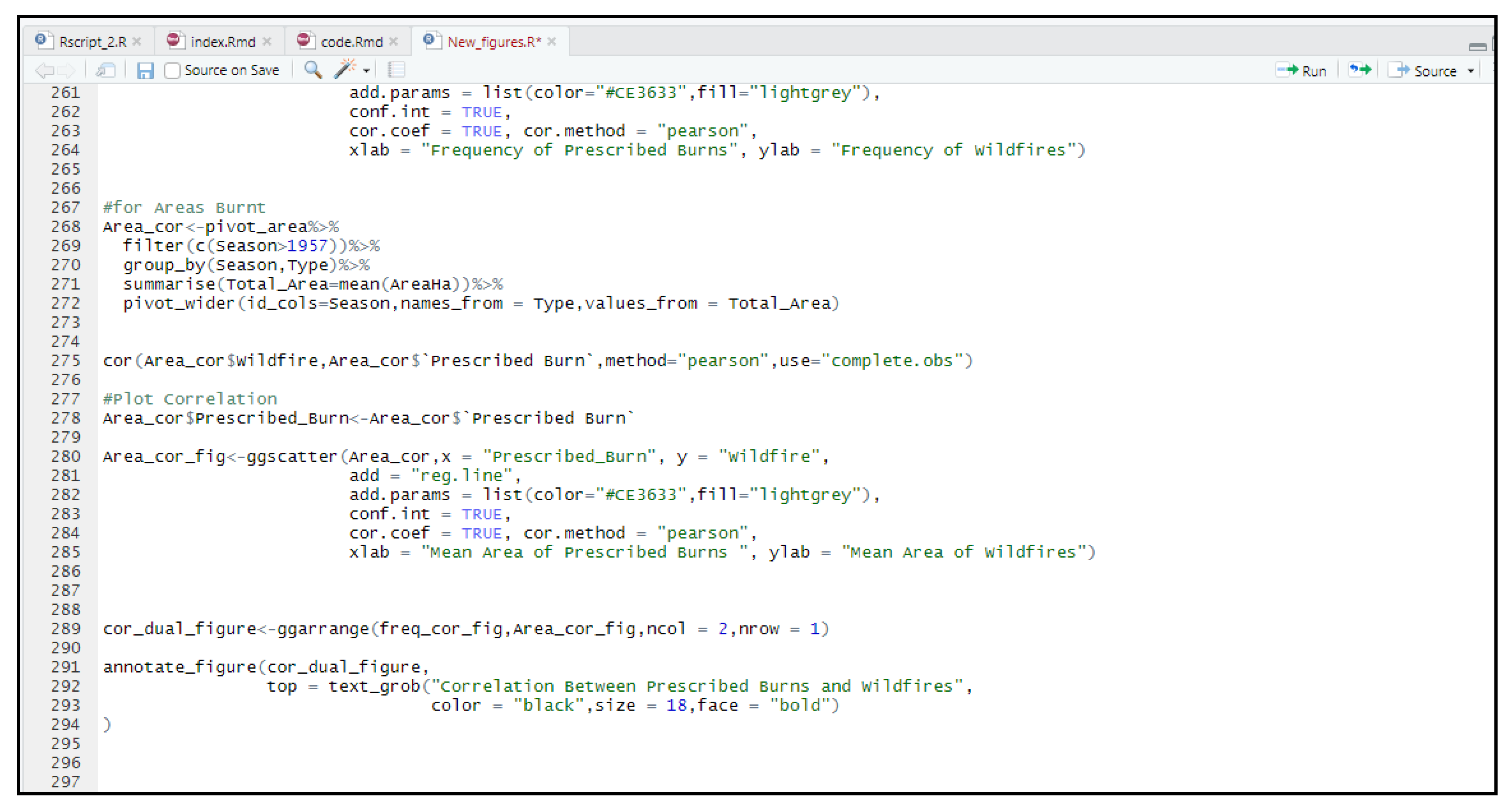
2.3.2. Correlation between Bushfires and Prescribed Burns

One of the objectives of this study is to examine the relationship between prescribed burns and bushfires to assess whether prescribed burns assist in reducing bushfire danger in NSW. This study used a similar approach to a previous study [45] that used a correlation analysis to determine the relationship between prescribed burns and bushfires. The principal behind using a correlation analysis in this case relies on the hypothesis that if prescribed burns decrease bushfire risk, then either the frequency or the burnt area of the fire will be negatively correlated between these two types of fires. The data frame previously imported into R (see Figure 4) has been used to perform a bivariate Pearson correlation, which produces a sample correlation coefficient (r), a commonly used to measure the strength of a linear relationship between two variables [46]. Pearson’s correlation between two variables x and y (prescribed burns and bushfires in this case) from n observations, is defined as [47]:
p = i = 1 n ( x i x ¯ ) ( y i y ¯ ) [ i = 1 n ( x i x ¯ ) 2   i = 1 n ( y i y ¯ ) 2 ] 1 / 2
where x ¯ and y ¯ are the mean values of x and y. In this study, x and y are representatives of prescribed burns and bushfires data, respectively.

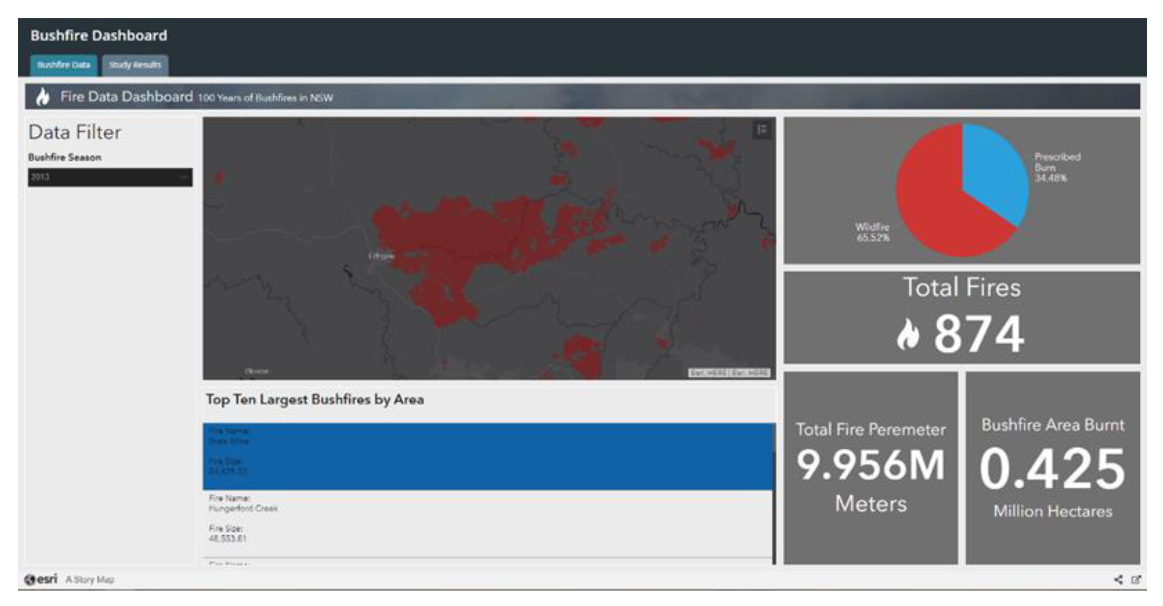
2.3.3. GIS Dashboard and Interactive Plots

This study’s data and results have been published in an online GIS dashboard that is open to the public. While most of the studies in the literature offer only an exclusive or limited access to the data used and all of its results, this study adopts an open data approach. The purpose of this dashboard is not only to produce the highly important insights of this study, but also to promote a freely accessible bushfire information platform that will allow both practitioners and decision-makers to reuse and redistribute the study’s data and results.
The plots that have been published on the online platform were first created in a static form with R, using different R libraries such as Tidyverse and grouper. Once the static plots were created, they were converted into an interactive html format, which was later published on Plotly and embedded in the dashboard.

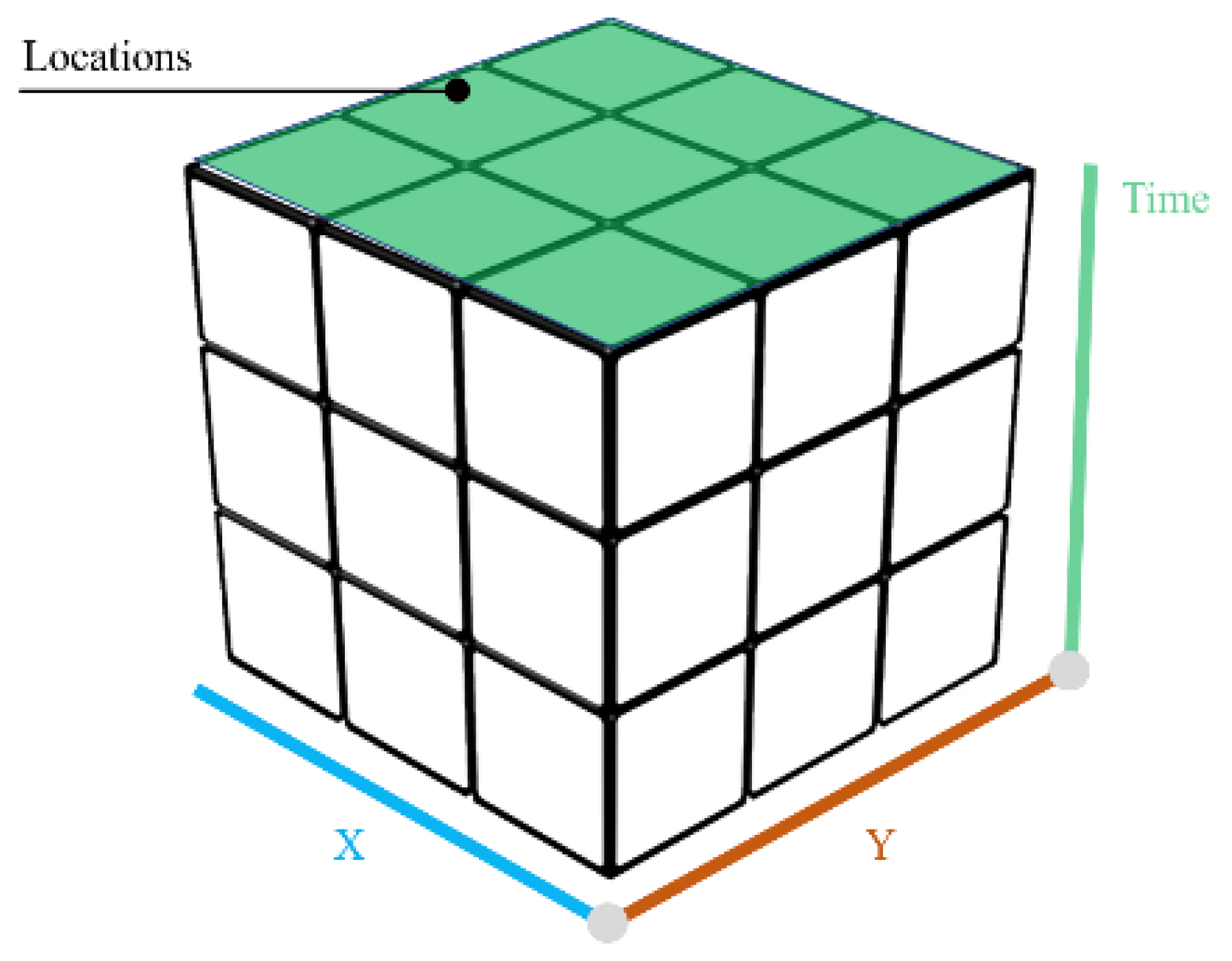
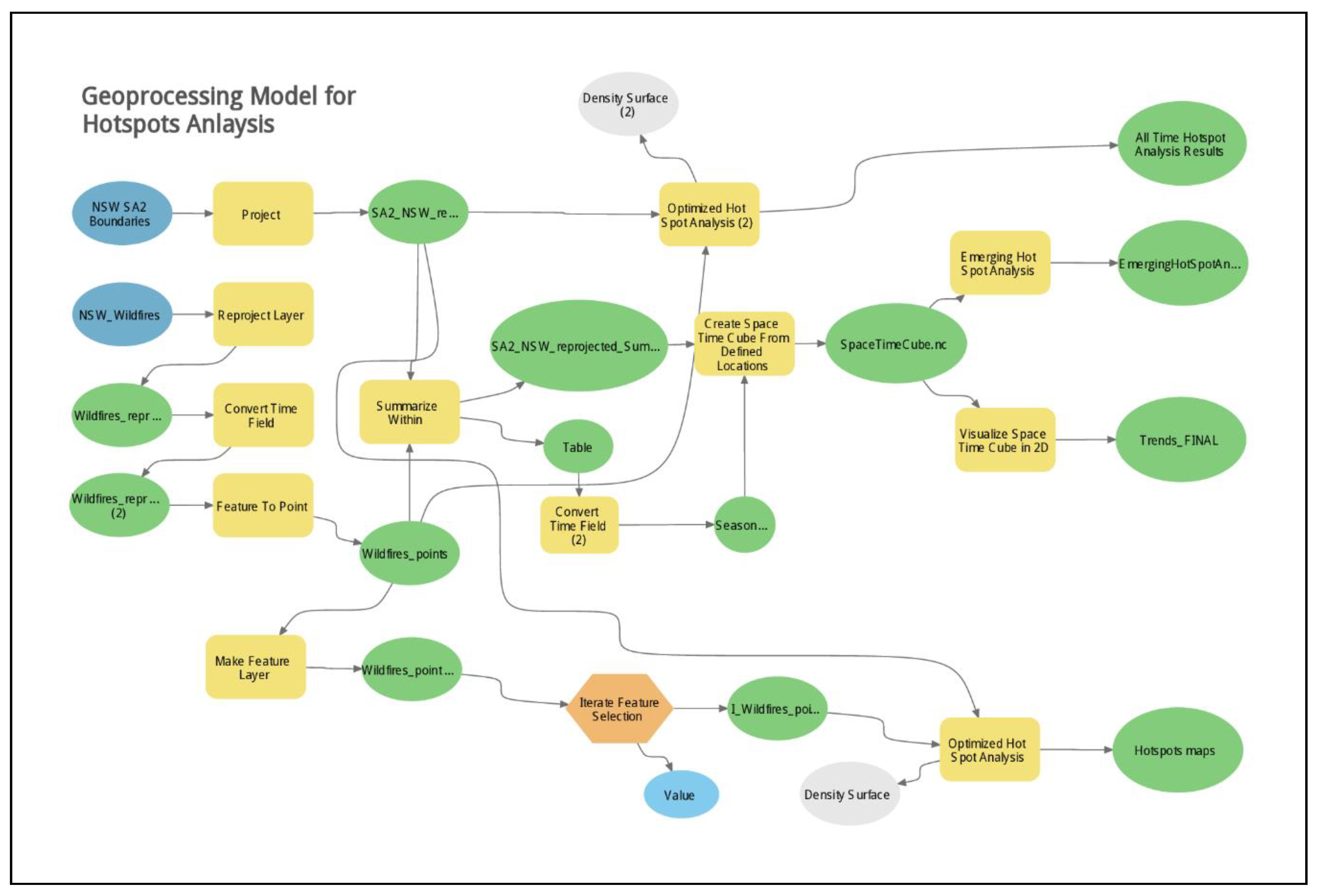
2.4. Spatio-Temporal Patterns of Fires

GIS are commonly used in the literature as a tool to analyse spatio-temporal patterns [37,48]. In accordance, this research uses a GIS approach to identify bushfire patterns over time. As mentioned, the dataset used in this research is a vector layer containing the fire boundaries of all the recorded fires in NSW since 1900, and as a result, there are numerous polygons that overlay each other. Compared to change detections in raster layers, there are fewer methods available for analysing spatio-temporal patterns in vector layers [49,50]. However, despite some of the limitations of vector GIS data, there are different methods for analysing spatial patterns over time [49]. The method in this analysis is based on similar analyses used in the literature [51,52,53] that used the Getis-Ord G i hotspot analysis, a spatial autocorrelation method that is used for evaluating clustering, randomness and fragmentation of spatial patterns [52,53,54].

2.4.1. Hotspot Analysis

The hotspot analysis required an additional overlaying polygon layer, divided into defined areas, to be added to the analysis to aggregate the total number of fires and their size within a particular area. To assess the best practice for defining such an area, two methods from the literature were considered. To use any of the two methods (Figure 5), the polygon fire data set was converted into points using ArcGIS Pro’s “Feature to Point” tool. Each point represents the centroid of each fire polygon.
According to Method 1, a square/hexagon grid is overlayed on top of the points. Then, all the points that fall within each grid cell are aggregated and counted. Based on the literature, it is more common to use a 1 km2 cell-sized grid for relatively small study areas [33,55], and a 5 km2 grid for larger study areas [56].
According to the Method 2 [40,51], the points are aggregated to an overlaying polygon of either statistical areas or municipalities, rather than a fixed grid. In order to be able to identify the regions where the hotspots occur, it was decided to adopt Method 2 (Figure 5) [40,51] by overlaying statistical area level 2 (SA2) polygons [57] on top of the fire points. This methodology was chosen in order to be able to associate bushfire patterns to municipal jurisdictions, rather than to a geographical hexagon/square grid. Size 2 statistical areas [58] were chosen, since they are the closest in size to the 5 km2 grid, suggested by Kwak [56] for large study areas such as NSW. After aggregating the points into the SA2 polygons, ArcGIS Pro’s “HotSpot Analysis” tool was used to calculate the Getis-Ord G i statistic, which results in a z-score and p-value that identify where features with either low or high values cluster spatially [59]. In other words, for an area to be a statistically significant hotspot, it needs a high value of bushfire frequencies and will be surrounded by other areas with high values of frequency. The G i local statistic is defined by Getis and Ord [59] as:
G i = j = 1 n w i , j x j X ¯ j = 1 n w i , j S     [ n   j = 1 n w i , j 2 ( j = 1 n w i , j ) 2 ] n 1
where x j   is the attribute value for feature j , w i , j is the spatial weight between feature i and j , and n is equal to the total number of features In addition, X ¯ and S are calculated as demonstrated below:
X ¯ = j = 1 n x j n
S = j = 1 n x j 2 n ( X ¯ ) 2
In this paper, the attribute values of bushfires are used so that the patterns of hotspots and coldspots can be extracted. As G i is a z-score, applying G i to each neighbour leads to a z-score for each pixel. In GIS domain, a low z-score obtained for a feature indicates that the neighbours of that feature have low values [53].

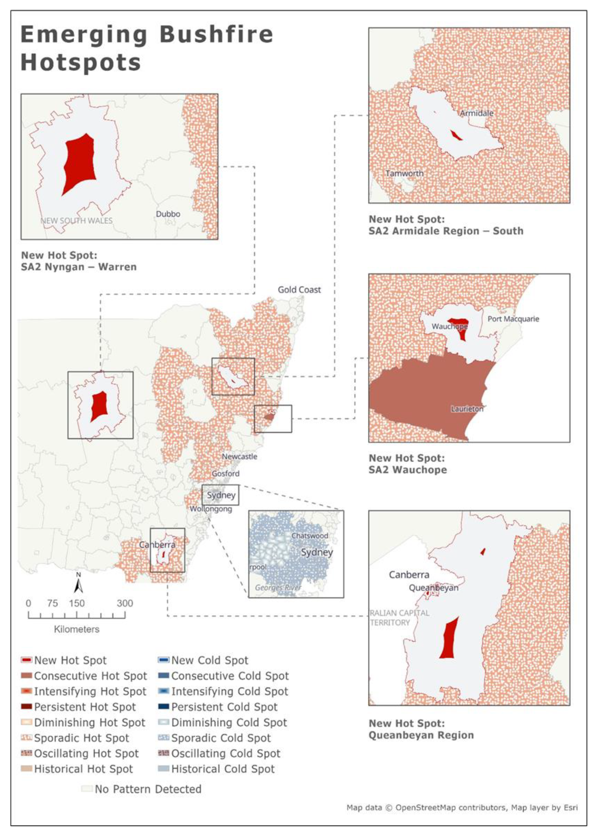
2.4.2. Emerging HotSpot Analysis

As for identifying temporal patterns, ArcGIS Pro’s “Create Space Time Cube from Defined Locations” tool was used to analyse the spatio-temporal trends. This tool uses time-stamped point features and converts them into a net-CDF file data cube of bins, where each bin’s values are measured across time and space using the Mann–Kendall statistic [60,61] (Figure 6). The Mann–Kendall test uses the following statistic [62]:
S = i = 1 n 1 j = k + 1 n sin ( x j x i )
If S > 0 , then later observations in the time series tend to be larger than those that appear earlier in the time series, while the reverse is true if S < 0 . The variance of S is given by:
v a r = 1 18 [ n ( n 1 ) ( 2 n + 5 ) t f t ( f t 1 ) ( 2 f t + 5 )   ]
Each bin within the data cube contains a count of the data value collected at each bin location for the specified timestamp. In this research, the space-time cube method was applied to fire data so that the spatio-temporal pattern of the concentration of fire could be detected.
After creating the space-time cube, ArcGIS Pro’s “Emerging Hotspot” tool was used to visualise the results of the space-time cube in a 2D map. The emerging-hotspot analysis tool is able to then identify hotspots and coldspots over time, and categorises these as new, consecutive, intensifying, persistent, diminishing, sporadic, oscillating, and historical hot and coldspots [63].
Once the methodology was set, a model was built using ArcGIS Pro’s “ModelBuilder” tool (Figure 7) to create a streamlined geoprocessing analysis, which allowed us to re-use the model in the future and reproduce results in case the data is updated. The results of this model included the following: (1) A hotspot analysis of all the aggregated bushfires in NSW; (2) 10 individual hotspot maps for each year between 2010 and 2020 to visualise the change in hotspots over time; (3) an emerging-hotspot analysis based on a space-time cube to identify new hotspots; (4) a trend map to visualise which areas experienced a positive/negative trend in the frequency of bushfires.

3. Results

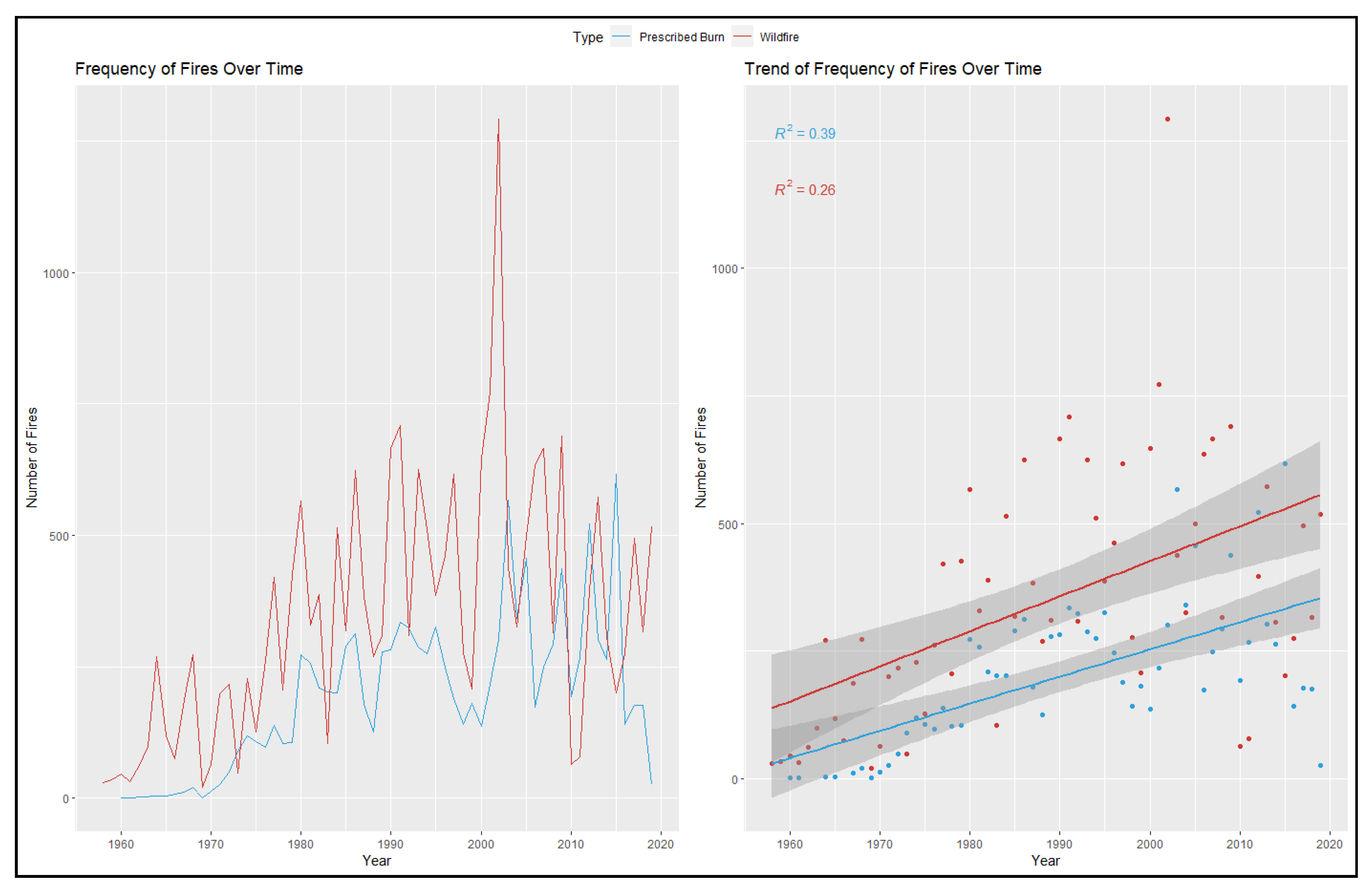
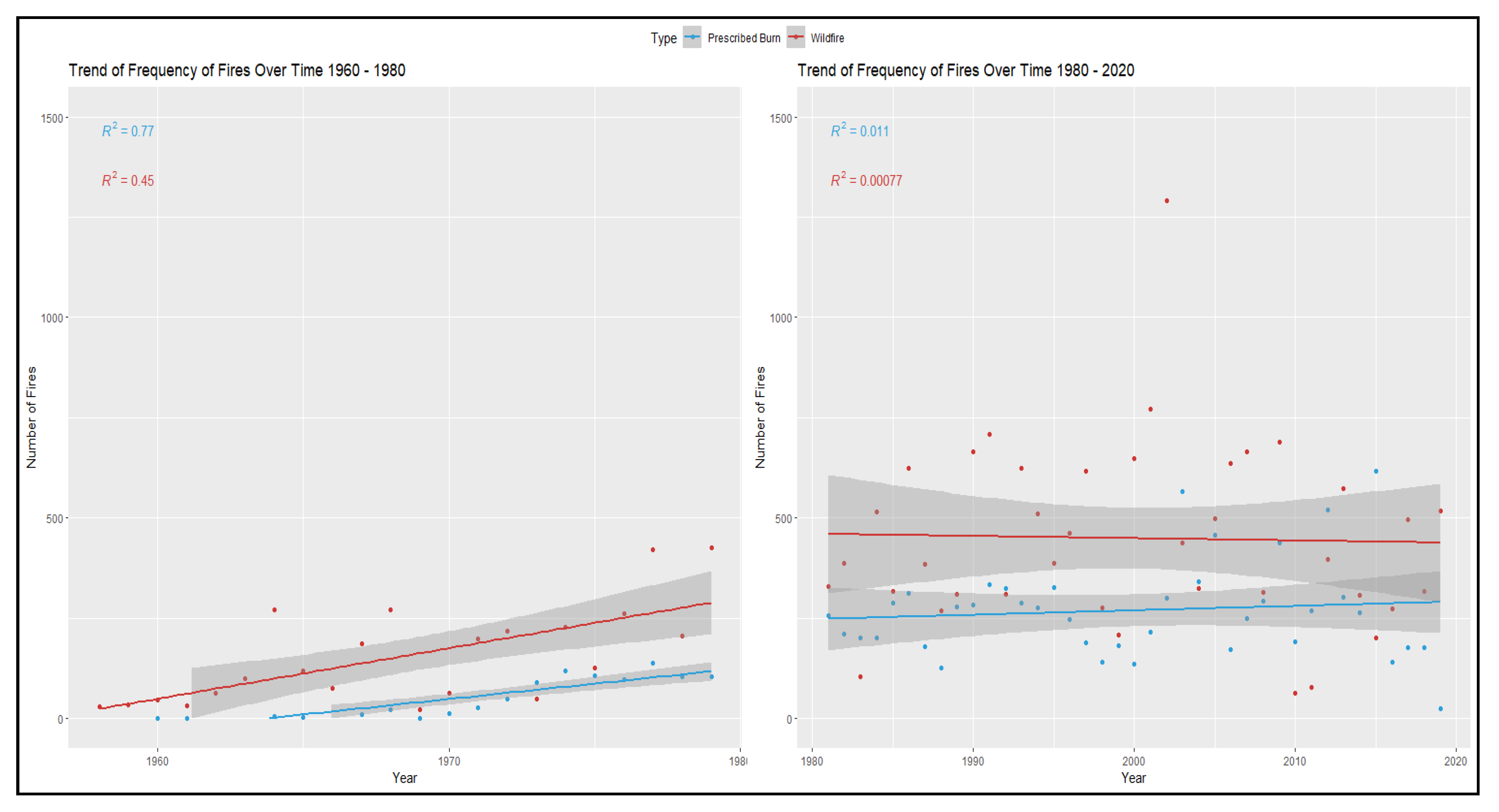
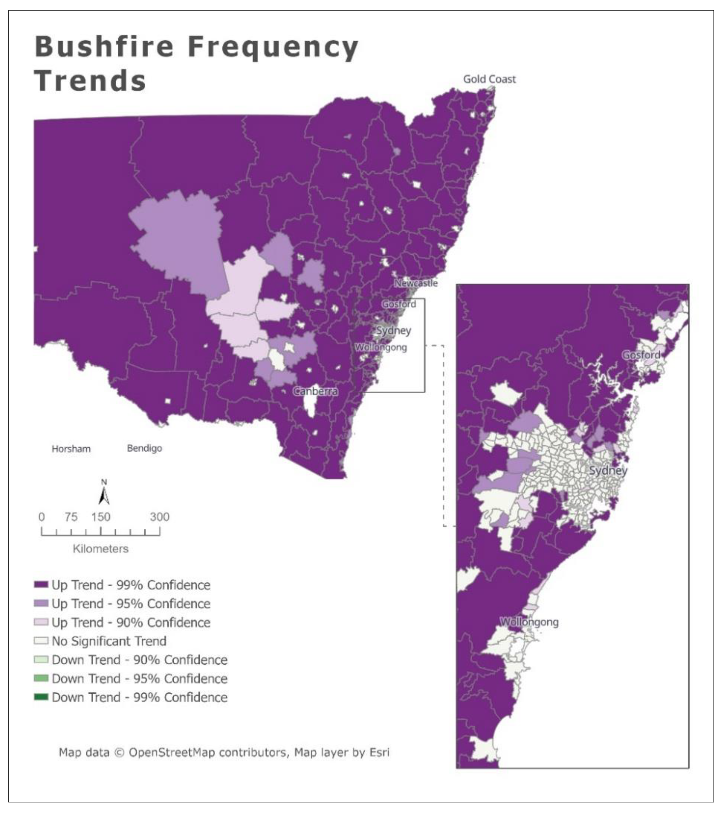
3.1. Increase in Fires over Time

A generalised linear model was developed to examine whether bushfires and prescribed burns have increased over time, because an increase in the frequency of fires does not necessarily mean an increase in the burnt area and vice-versa. For example, a possible option is that the frequency is increasing, but the size of fires is decreasing, resulting in a smaller total of burnt area. This is why the generalised linear model was used to assess both the frequency and the area of the fires.
According to the literature, extreme fire events, in which the total burnt area is higher than the average, occur in Australia at least once a decade [1,5]. Plotting the data suggests that a similar pattern occurs in NSW, which can be seen in the highly fluctuated results (Figure 8). As seen in Figure 8, the scattered data is highly variable. While it is common to detect and remove outliers to improve statistical models, it is important to understand that in this case, extreme fire events are outliers that are a crucial part of the natural bushfire cycle [1,5].
As an alternative to treating the extreme fire events as outliers and removing them from the analysis completely, all the extreme fire events were analysed separately. However, in order to separate the extreme fire events from data, it was first crucial to know the minimum area that defines a bushfire as an extreme fire event.
In the U.S., extreme fire events, or megafires, are defined as bushfires with a minimum area of 40,500 hectares; while in Europe, the size is smaller, with a minimum of 1000 ha [64]. Using any of these definitions to identify extreme fire events in NSW is not applicable to this study’s data, since the median area of fires in this dataset is already much higher than the U.S. definition. Consequently, extreme events were identified by detecting statistical outliers [10], based on a classical boxplot. These values were then extracted into an additional data frame to determine if there was also an increasing trend in extreme fire events alone. The results (Table 1) suggested years when extreme fire events occurred with a mean burnt area larger the 1887 ha. Figure 9 was produced using only the values in Table 1, in order to examine if there was a pattern of change in the burnt area of extreme fire events over time. Figure 9 does not indicate a pattern of increase or decrease in the area burnt in extreme fire events; however, the results (Table 1, Figure 9) suggest that extreme fire events occur in cycles in New South Wales, similar to the fire pattern described by Cheney [5] and Payne [1].
Regarding the frequency of fires, Figure 10 was produced to examine if the frequency of fires is increasing over time. The results indicated that the frequency has been steadily increasing over time since the 1960s. However, when examining the figure, it appears that there is much more variability in the data between 1980–2020 compared to 1960–1980.
Figure 11 was created to examine if the trend was more significant between 1960–1980 compared to 1980–2020. The results show an increasing trend of the frequency of fires between 1960–1980; however, this could be a result of less available data between those years. In both Figure 10 and Figure 11, the variability in the results was higher among bushfires (wildfires) compared to prescribed burns. A possible reason for these results could be the origin of the fires. Compared to prescribed burns, which are man-made fires that are scheduled by fire agencies in different intervals, bushfires depend on different weather conditions such as wind and rain. Changes in these factors are likely to increase the randomness in the frequency of fires in each bushfire season.

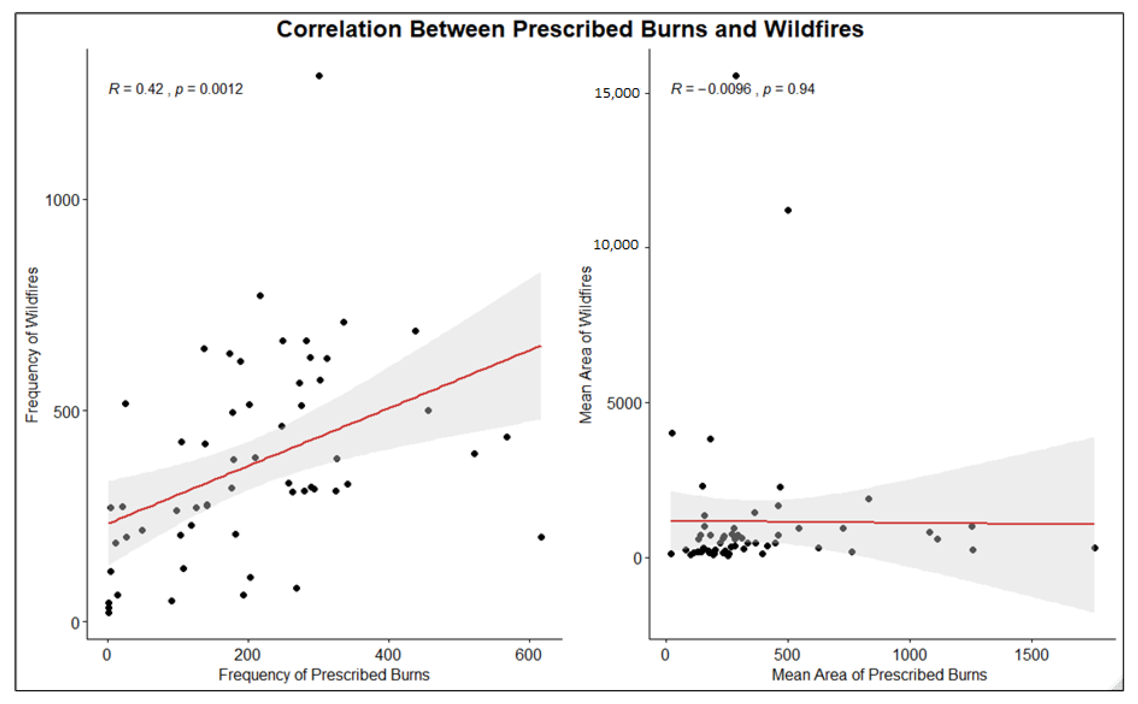
3.2. Pearson’s Correlation between Bushfires and Prescribed Burns

Figure 12 was created to explore the possible relationship between bushfires and prescribed burns by performing a bivariate Pearson’s correlation [46], in alignment with the literature [45]. As mentioned before, the practice of prescribed burning is based on the hypothesis that intentionally burning areas that are abundant in forest fuels will decrease the frequency, area and intensity of fires [13,14]. If this hypothesis is true, the results should indicate negative correlation between bushfires and prescribed burns in both frequency and burnt area. However, the correlation coefficient (r) in Figure 12 suggests that in the case of the frequency of fires, there is a positive correlation between prescribed burns and bushfires, i.e., the frequency of bushfires is growing in respect to the frequency of prescribed burns, and vice versa. On the other hand, examining the correlation between the area of prescribed burns and bushfires reveal different results. As seen, the value of the correlation coefficient (r) is negative and very low, which indicates that there is no correlation between the area of prescribed burns and bushfires (wildfires). While it was not within the scope of this study to identify the reasons for these results, some of possible reasons are discussed in the Discussion section of this study.

3.3. Spatial Clustering of Bushfire Frequency

As opposed to the previous sections, which examined the bushfire patterns and their relationship with prescribed burns, the spatial-clustering analysis only included bushfires. The results of the spatial-temporal patterns of bushfires are presented in the following maps, which were produced with ArcGIS Pro using the model described in Figure 7.

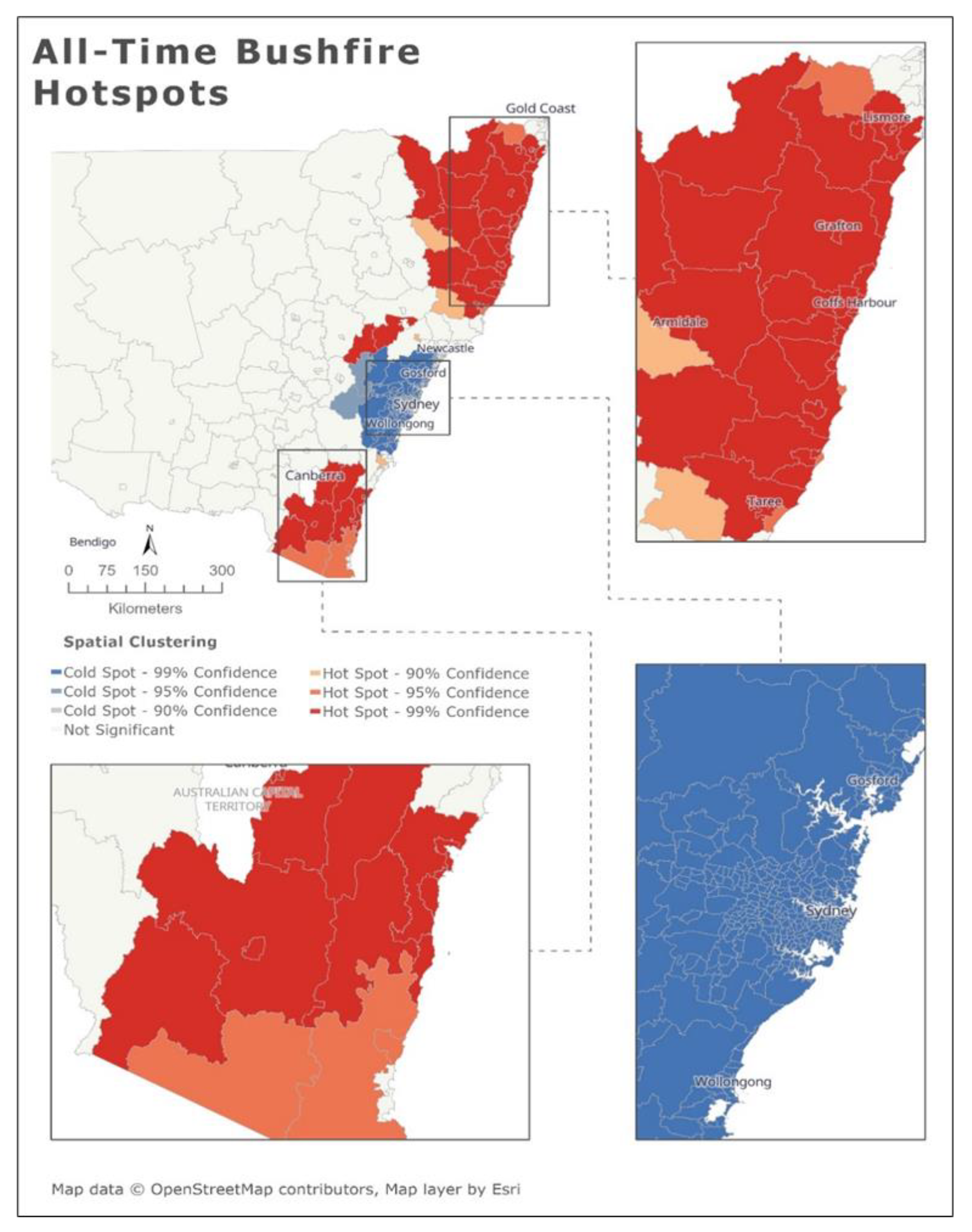
3.3.1. All Time Hotspot Analysis

At first, all the bushfire data was used to perform an optimised hotspot analysis, which calculated the Getis-Ord G i statistic values and reveals the spatial clustering of bushfire frequency for each level 2 statistical area in NSW. Figure 13 is map of New South Wales and includes the boundaries of all the level 2 statistical areas in the state. Coldspots (blue) and hotspots (red) can be seen in the map in three different colour variants; the darker the variant, the higher the confidence level of the G i statistic. Figure 13 shows a spatial clustering of high values (hotspots) in northeastern and southeastern NSW along the Northern Rivers, North Coast and South Coast regions, while a spatial clustering of low values (coldspots) can be seen around the Sydney metropolitan area, along the Central Coast and Illawarra regions. One explanation for these results could be the geographic and topographic characteristics of these areas. The coldspots in Figure 13 are concentrated around highly populated urban areas. These highly developed areas obviously do not have as much vegetation that can burn, especially compared to the hotspot areas of the Far South Coast and Far North Coast of New South Wales, which are abundant in dense forest areas.

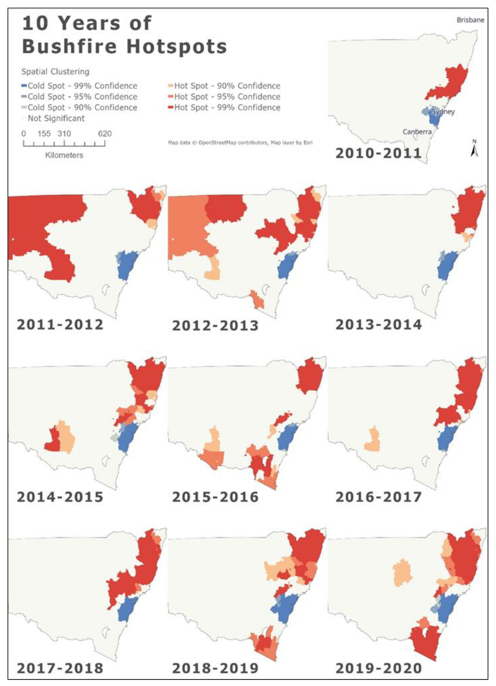
3.3.2. Bushfire Frequency Hotspots between 2010–2020

Figure 14 was produced to visualise the changes in the bushfire frequency hotspots in the 10 years preceding the catastrophic 2019–2020 bushfire season. Figure 14 shows how versatile bushfire location can be, and demonstrates how hotspots changed between 2010–2020. As in Figure 13, blue areas indicate bushfire coldspots, while red areas indicate hotspots. The figure reveals that, similar to Figure 13, the area around Greater Sydney, including Wollongong and the Central Coast, has been a bushfire coldspot in every one of the bushfire seasons between 2010–2020, while the location of bushfire hotspots seems to be changing more radically. Even though bushfire hotspots changed more radically than coldspots throughout this time period, the bottom half of Figure 14 could suggest a pattern of movement in bushfire hotspots between 2015–2020. During those years, hotspots seemed to move closer to the area of Greater Sydney, Australia’s most populated area.
In addition, Figure 14 might also suggest a pattern movement of the bushfire hotspots towards the area of Greater Sydney, especially between 2015–2020.
Figure 15, which was produced using the “Space Time Cube” (Appendix A) and the “Emerging Hotspot” tools, describes the change over time in fire frequency in each of NSW’s SA level 2 areas. ArcGIS Pro’s Emerging Hotspot tool uses a space-time cube to identify the change over time of different types of hot/cold spots, which, as described previously, are areas with significant spatial clustering. The results indicated that most of the areas are sporadic hot/coldspots, which are areas where hot/cold spots disappear and reappear over time. Sporadic coldspots can be seen in the Sydney metropolitan area around the Sydney Harbour together with diminishing coldspots, that is, areas that become less of a coldspot over time. On the other hand, there is a significant presence of sporadic hotspots in the NSW South Coast and North Coast regions. Most importantly, the results have identified four new hotspots of bushfire frequency in NSW, which are areas that have never been a hotspot until the recent 2019–2020 bushfire season, the final time stamp in the dataset. These statistical areas are Nyngan—Warren, Queanbeyan Region, Armidale Region—South and Wauchope.

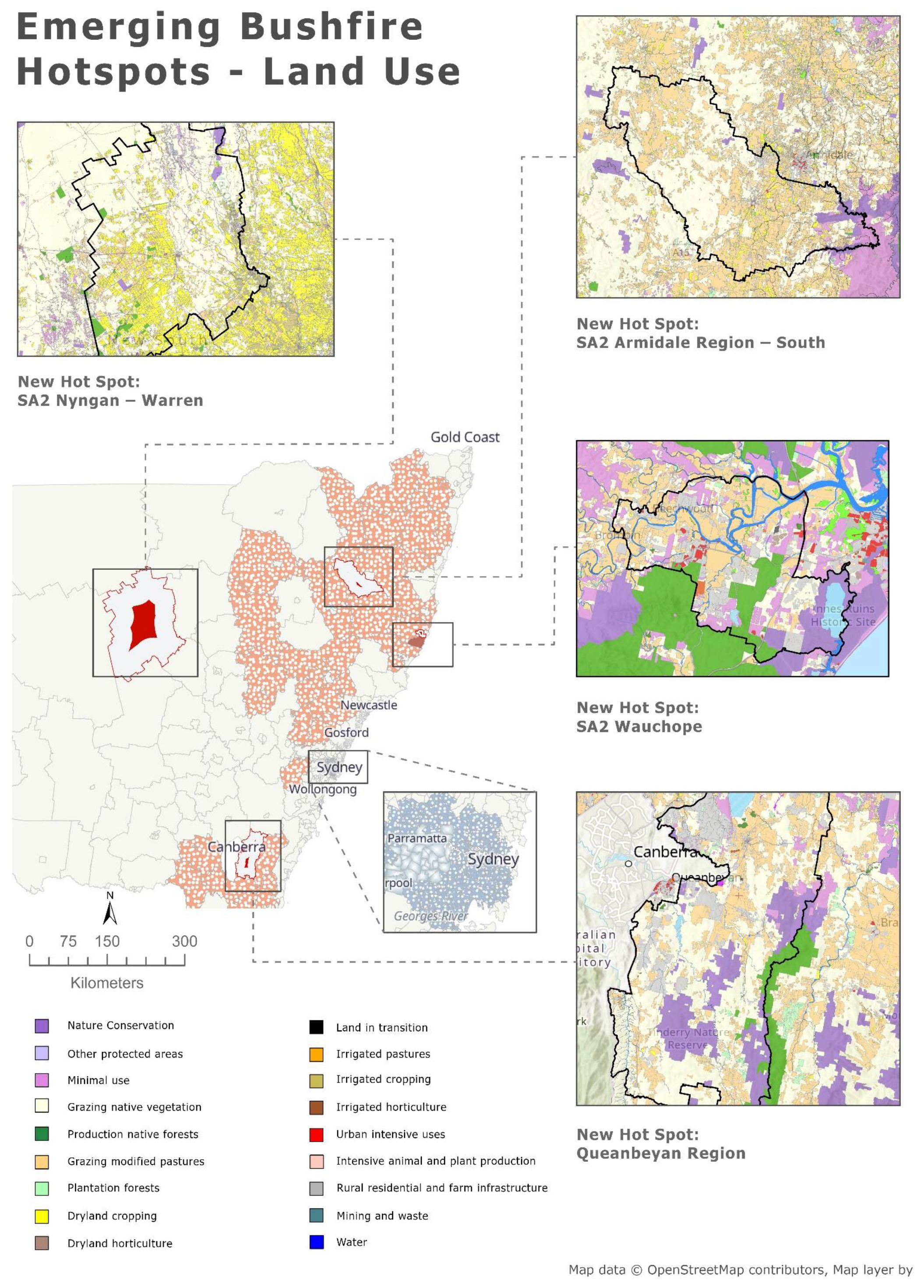
3.4. Land Use in Hotspots

Figure 16 was created to examine the geographical characteristics and land use of the four new hotspots identified in New South Wales in Figure 15. As seen in Figure 16, the new identified hotspots are scattered throughout the State of New South Wales and are located in entirely different topographical divisions. In fact, the hotspots represent together almost all the state’s topographical divisions, including the coast, the Great Dividing Range, the Snowy Mountains and the Western Plains. The contrasting topographical divisions of each one of the hotspots is likely to be the reason for the versatility in the land use among these statistical areas, including dryland cropping, grazing native vegetation, production and plantation forests, native conversation and intensive urban use. The combined area of all the new hotspots is about 2.7 million hectares, and they are populated with nearly 40,000 residents in at least 13,000 dwellings [65].

Bushfire Frequency Trends

Another method to visualise the space-time cube of this analysis in 2D is a trend map. Figure 17 was produced using ArcGIS Pro’s “Visualise Space Time Cube” tool to display the trends of change in the frequency of bushfires in each statistical area level 2 in New South Wales over time. This tool determines the trend of values in each location using the Mann–Kendall Statistic and displays the trend on a 2D map. The figure is based on two major colours, green and purple, which indicate a downward or upward trend, respectively. Both colours are divided into variations; the darker the colour, the higher the statistical confidence level. As seen in Figure 17, most of the statistical areas (SA2s) in New South Wales have experienced an increase in the frequency of fire in the last 100 years, with a 99 percent confidence level. As also seen in Figure 13, Figure 14, Figure 15 and Figure 16, there is a different trend in the metropolitan areas of Greater Sydney, the Central Coast and Wollongong compared to regional New South Wales. In this case, the figure indicates that in most of the statistical areas within these metropolitan areas, there was no significant trend of increase or decrease in the frequency of bushfires. Once again, this could be a result of the urban characteristics in these areas. The enclosed map of Greater Sydney (Figure 17) demonstrates there was no significant trend within the highly developed inner city, compared to the regional outskirts, where an increasing trend was present in bushfire frequency.

3.5. Bushfire Dashboard

After all the figures and maps were produced, all the outputs were uploaded to the hosting servers of GitHub, Chart Studio and ArcGIS Online. ArcGIS Online’s “Sites” tool was used to create a publicly available online platform. The online platform allows its users to access all the data that was used throughout this study, scroll through a story map that visualises the methodology used for this study, and most importantly, access an interactive dashboard. The dashboard (Figure 18 and Figure 19) compromises two tabs. The first tab (Figure 18) allows users to explore the entire dataset used in the study and interactively calculate different statistics based on location, year, etc. The second tab (Figure 19) allows users to access interactive versions of all the figures in the Results section of this study. The dashboard, demonstrated in Figure 18 and Figure 19, is publicly available and can be accessed through this link: https://tinyurl.com/y2bdp4h8.

4. Discussion

The objective of this study was to understand how bushfire patterns have changed in New South Wales by conducting a spatio-temporal analysis of 100 years of bushfire data. The study used three key analysis techniques to answer its research questions, and used data-analysis and spatial-analysis software such as R and ArcGIS Pro.
First, generalised linear modelling was applied on the data to assess whether there was a pattern of change in the size and frequency of bushfires in New South Wales in recent decades. The literature review has shown that bushfires have played a major role in Australia’s eco-system for millions of years and are vital for some of its flora and fauna [2,3,4]. However, an increase in the frequency and the intensity of fires may have devastating results [2,3,4]. Based on the literature [6,9,10,36,39], the hypothesis of this study was that bushfires have been increasing in New South Wales in the last decades, similar to the trend observed throughout Australia. The results have shown this hypothesis to be true. While the results indicated that there was a trend of increase in the frequency of bushfires and prescribed burns since the 1960s (Figure 10), they did not indicate a trend of change in regard to the size of the burnt area (Figure 8). Further analysis revealed (Figure 11) that the variability of the frequency of fires was higher between 1980–2020 compared to 1960–1980. As a result, the trend of increase in the frequency bushfires appears to flatten after 1980. It is not within the scope of this study to assess what caused these results. This part of the study also examined the patterns of extreme bushfire events, which according to the literature occur in Australia once every one or two decades [1,5]. Extreme fire events in New South Wales were identified by detecting statistical outliers, based on a classical boxplot. The results (Table 1, Figure 9) identified seven extreme fire events with a mean area larger than 1887 ha.
Another aim of this study was to examine whether prescribed burning is an effective tool to reduce bushfire risk. To do so, a bivariate Pearson’s correlation test was performed according to each fire’s type (prescribed burn/bushfire) (Figure 12), to measure the strength of the linear relationship between two variables [46]. The hypothesis behind using a correlation test was that if prescribed burning reduces bushfire risk, then the results should indicate a negative correlation between bushfires and prescribed burns in both frequency or burnt area. The principal of using a correlation test to examine the relationship between bushfires and prescribed burns originated from Pollet [45], who also used a correlation test to assess the effectiveness of prescribed burns; however, in that study, they analysed the correlation between pine tree characteristics and fire severity, while our study analysed the direct relationship between bushfire size and frequency to prescribed burns. Therefore, the results of Pollet [45] and Omi (2002) cannot be compared with this study.
According to Figure 12, there is a positive correlation between the frequency of bushfires and prescribed burns, yet there were no significant results regarding the size of the area of the fires. In NSW, prescribed burns are used as a method for clearing forest fuels and preventing extreme bushfire events, so we assumed that the positive correlation between the frequency of bushfires and prescribed burns is a result of two possible scenarios. First, the number of bushfires has increased, and as a result, fire authorities in NSW have increased the number of prescribed burns as a preventative action. Second, the increase in prescribed burns over time has led to an increase in the number of bushfires. Even though prescribed burns have gone out of control in the past, scenario two is less likely to be the reason for the positive correlation. Determining the reason for this correlation is not within the scope of this study; therefore, this is suggested as the direction of future studies based on this research. As mentioned, the correlation analysis of this study also examined a possible correlation between the size of the burnt areas from prescribed burns and bushfires. The result (Figure 12) was a correlation coefficient (r) with a low negative value, which does not indicate a correlation. This means that based on this study’s results, it is impossible to determine if prescribed burns effectively reduce bushfire risk. Thus, further analysis is needed with more sufficient data to determine the relationship between prescribed burns and bushfires.
The last step of this study was the spatio-temporal analysis, which examined how geographic patterns and spatial clusters of bushfire frequency have changed over time and space in New South Wales. As described, the data used for this study were originally in a GIS polygon vector layer that contained all fire boundaries in NSW since 1900. Despite the limitations of using vector GIS data for a spatio-temporal analysis [49,50], this study developed a spatial framework to overcome these limitations. Figure 7 was developed using ArcGIS Pro’s ModelBuilder and describes the all the geo-processing tools that were used for populating the results of this study. The logic behind using a streamlined model, rather than running different geo-processing tools separately, is that the entire process could be redone in case the bushfire dataset is updated in the future, and would also allow other practitioners to imitate this study’s results for future bushfire research and further analysis.
The spatial framework of this study (Figure 7) was developed according to the elements of previous hotspot analyses in the literature [40,51,52]. However, as opposed to past studies, this study’s framework was developed to specifically address the authors’ intention to answer the specific research questions of this study. As opposed to the common practice in the literature to convert polygons into points, and then aggregate them into either a hexagonal or fishnet grid [33,55,56], this study’s spatial framework has aggregated bushfire centroids to level 2 statistical areas in order to be able to associate bushfire patterns to municipal jurisdictions, rather than geographical grid cells.
The results of the hotspot analysis (Figure 13) identified Greater Sydney and its surrounding areas as bushfire frequency coldspots, and the Far North Coast and Far South Coast regions as all-time bushfire hotspots. Figure 14 was created to examine the change in bushfire frequency hotspots in the 10 years preceding the 2019–2020 bushfire season. The figure suggests that there could be a pattern of movement of hotspots towards the Sydney metropolitan area; however, additional data and information are required to confirm this.
The emerging-hotspots analysis (Figure 15) identified four new statistical areas that became fire hotspots in the 2019–2020 bushfire season; these statistical areas are Nyngan—Warren, Queanbeyan Region, Armidale Region—South and Wauchope. Figure 15 reveals a number of patterns of hotspots that emerged in the 2019–2020 bushfire season. First, three out of four of these new hotspots (Queanbeyan Region, Armidale Region—South and Wauchope) are located in vegetated areas, while Nyngan—Warren is located in the centre of NSW, a less-vegetated area characterised by an extremely hot and dry climate (Figure 16). Second, Figure 16 shows that except for Nyngan—Warren, all other emerging hotspots are located within close proximity to population centres such as Port Macquarie, Armidale and Canberra. Considering that the frequency of bushfires is increasing in NSW according to both predictions and the results of this study, the impacts on the communities, environment and vulnerable wildlife within these statistical areas may be devastating in the future. Third, Nyngan—Warren is the only new hotspot that is not surrounded by other types of hotspots. This could suggest that bushfires will be present in the area in the future more than they have been in the past. Nevertheless, examining why exactly these areas have become bushfire frequency hotspots in the 2019–2020 bushfire season was not within the scope of this study.
As shown in Figure 17, there was a trend of increase in the frequency of fires, with a 99% confidence, in most of the level 2 statistical areas in NSW, except in metropolitan areas such as Sydney. This reinforces the hypothesis suggested by the literature that bushfires are increasing in NSW, as well as overall in Australia. It is important to note that numerous studies point out that the increase in bushfire frequency is a direct result of climate change [6,9,10], but it was not within the scope of this research to assess what the cause of this increase, and the authors recommend this topic as a future direction for this research.
As mentioned above, all the findings of this study were uploaded into an online platform that also includes an interactive dashboard. To date, the developed dashboard of this study (Figure 18 and Figure 19) is unique because it enables users to browse through more than 100 years of bushfire data. The dashboard also gives users the ability to download the raw data of the study, as well as its results, and therefore can be of great value for additional bushfire research and decision-making.
To better understand the reasons for the detected patterns, one of the future directions of this research is recommended to be based on using artificial intelligence to process and analyse big data using various data types from web services. Methods such as the ones proposed by Berner [66,67] can be further investigated to be used for this purpose.
The authors recommend overcoming the following limitations for future studies based on this research:
  • Lack of enough data before 1957.
  • Low accuracy of the data relevant to the boundaries of the fires for early data in the century.
  • Lack of provision of the intensity attribute for the fires (e.g., “light” fires in large areas compared to “intense” fires in small areas). Such intensity data can help to explore whether prescribed burns have reduced the fire intensity but not the area/frequency.

5. Conclusions

The goal of this study was to conduct a spatio-temporal analysis on more than 100 years of historical bushfire data to shed a light on how bushfire patterns have changed in the last 100 years.
The study used a two-step approach to analyse the data and achieve its objective. The first step focused on statistical data analysis and used methods such as generalised linear modelling and a Pearson’s correlation test. In the second step of the analysis, GIS techniques such as hotspot analysis were applied to the temporal data to identify the spatial and temporal changes of bushfires.
As mentioned in the introduction, three research questions were developed to achieve the goal of this study. The first one questioned whether there has been a trend of increase in bushfires in recent decades. The results indicated that the frequency of bushfires in New South Wales has increased; however, they could not indicate whether the size of these fires is also increasing. The second question analysed whether prescribed burns are an effective tool for reducing bushfire risk by conducting a correlation analysis. According to the results of this study, it is impossible to determine whether prescribed burns have a significant impact on reducing bushfire risk bushfires. Therefore, the authors recommend conducting further analysis with more sufficient data to determine if prescribed burns affect the size and frequency of bushfires.
Finally, the study examined if the frequency of bushfires was spatially clustered over time, and if so, how the clustering was different compared to the 2019–2020 bushfire season. Using different hotspot-analysis methodologies, the study found four new statistical areas that became hotspots of bushfire frequency during the 2019–2020 bushfire season; namely, Nyngan—Warren, Queanbeyan Region, Armidale Region—South and Wauchope. In addition, the findings of this study also suggest that there is a possible pattern of movement in bushfire frequency hotspots towards the highly populated area of Greater Sydney. Since this pattern of movement is not absolute, and due to the potential threat of bushfires moving towards dense urban areas in the future, the authors strongly recommend future research in that field.
The fact that this study used statistical areas to identify bushfire frequency hotspots in New South Wales also means that the findings of this research can be potentially used as a baseline for future research that will examine how bushfire hotspots may affect different socio-economic characteristics of the communities living within their boundaries. In a smart-city paradigm, these types of findings in this study will be of great importance for informed, data-driven decision-making by fire agencies on all levels, in order to preserve lives, natural resources and property. They will allow policymakers to specifically target urban and rural areas that are at greater fire risk. The authors recommend that further discovery research on the reasons behind the new hot spots should be considered to develop preventive/mitigation strategies in hot seasons across New South Wales, Australia.

Author Contributions

Conceptualization, M.V., S.S., C.P.; methodology, S.S., M.V.; software, M.V.; validation, M.V., S.S.; formal analysis, M.V., S.S.; investigation, M.V., S.S., C.P.; resources, C.P.; data curation, M.V.; writing—original draft preparation, M.V., S.S.; writing—review and editing, M.V., S.S., C.P.; visualization, M.V., S.S.; supervision, S.S., C.P. All authors have read and agreed to the published version of the manuscript.

Funding

This research received no external funding.

Data Availability Statement

The data sets used and generated can be found in the dashboard created in this study https://tinyurl.com/y2bdp4h8.

Conflicts of Interest

The authors declare no conflict of interest.

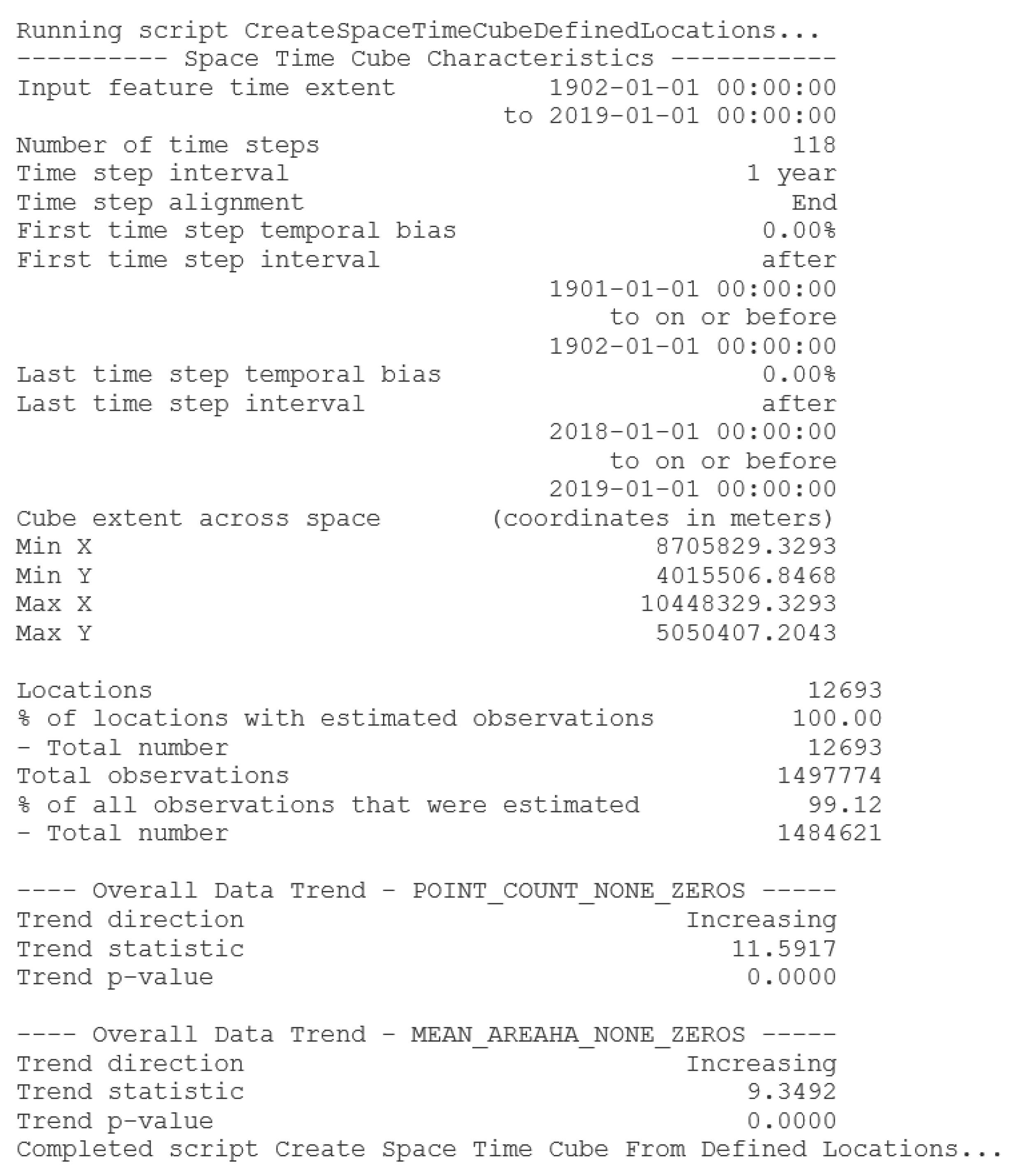
Appendix A. The space-time cube logfile.

Buildings 11 00037 g0a1

References

  1. Payne, J.S. Burning Bush: A Fire History of Australia; Henry Holt and Company, Inc.: New York, NY, USA, 1991. [Google Scholar]
  2. Gill, A.M.; Groves, R.H.; Noble, I.R. Fire and the Australian Biota; Australian Academy of Science: Canberra, Australia, 1981. [Google Scholar]
  3. Bradstock, R.A.; Cohn, J.S.; Gill, A.M.; Bedward, M.; Lucas, C. Prediction of the probability of large fires in the Sydney region of south-eastern Australia using fire weather. Int. J. Wildland Fire 2009, 18, 932–934. [Google Scholar] [CrossRef]
  4. Russell-Smith, J.; Yates, C.P.; Whitehead, P.J.; Smith, R.; Craig, R.; Allan, G.E.; Thackway, R.; Frakes, I.; Cridland, S.C.M.; Meyer, M.C.P.; et al. Bushfires ‘down under’: Patterns and implications of contemporary Australian landscape burning. Int. J. Wildland Fire 2007, 16, 361–377. [Google Scholar] [CrossRef]
  5. Cheney, N.P. Bushfire Disasters in Australia, 1945–1975. Aust. For. 1976, 39, 245–268. [Google Scholar] [CrossRef]
  6. Hasson, A.E.A.; Mills, G.A.; Timbal, B.; Walsh, K. Assessing the impact of climate change on extreme fire weather events over southeastern Australia. Clim. Res. 2009, 39, 159–172. [Google Scholar] [CrossRef] [Green Version]
  7. Hill, R.S. History of the Australian Vegetation: Cretaceous to Recent; University of Adelaide Press: Adelaide, SA, Australia, 2017. [Google Scholar]
  8. Dickman, C. Number of Animals Feared Dead In Australia’s Wildfires Soars To Over 1 Billion. Huffpost, Ed. The HuffPost, 7 January 2020. Available online: https://www.huffingtonpost.com.au/entry/billion-animals-australia-fires_n_5e13be43e4b0843d361778a6?ri18n=true (accessed on 22 January 2021).
  9. Hennesy, K.; Lucas, C.; Nicholls, N.; Bathols, J.; Suppiah, R.; Ricketts, J. Climate Change Impacts on Fire-Weather in South-East Australia. In Proceedings of the Joint AFAC/IFCAA Bushfire CRC Conference, Melbourne, Australia, 10–13 August 2006; East Melbourne, Vic.: Melbourne, Australia, 2005. [Google Scholar]
  10. Lucas, C.; Muraleedharan, G.; Soares, C. Outliers identification in a wave hindcast dataset used for regional frequency analysis. In Maritime Technology and Engineering; CRC Press: Cleveland, OH, USA, 2014; pp. 1317–1327. [Google Scholar] [CrossRef]
  11. Matthews, S.; Sullivan, A.L.; Watson, P.; Williams, R.J. Climate change, fuel and fire behaviour in a eucalypt forest. Glob. Chang. Biol. 2012, 18, 3212–3223. [Google Scholar] [CrossRef] [PubMed] [Green Version]
  12. Clarke, H.G.; Smith, P.L.; Pitman, A.J. Regional signatures of future fire weather over eastern Australia from global climate models. Int. J. Wildland Fire 2011, 20, 550–562. [Google Scholar] [CrossRef]
  13. Boer, M.M.; Sadler, R.J.; Wittkuhn, R.S.; McCaw, L.; Grierson, P.F. Long-term impacts of prescribed burning on regional extent and incidence of wildfires-Evidence from 50 years of active fire management in SW Australian forests. For. Ecol. Manag. 2009, 259, 132–142. [Google Scholar] [CrossRef]
  14. McCormick, B. Is Fuel Reduction Burning the Answer? Parliament of Australia: Canberra, Australia, 2002. [Google Scholar]
  15. Flannery, T. The Future Eaters: An Ecological History of the Australasian Lands and People; Grove Press: Greenwich Village, NY, USA, 2002. [Google Scholar]
  16. Bird, R.B.; Bird, D.W.; Codding, B.F.; Parker, C.H.; Jones, J.H. The “fire stick farming” hypothesis: Australian Aboriginal foraging strategies, biodiversity, and anthropogenic fire mosaics. Proc. Natl. Acad. Sci. USA 2008, 105, 801–14796. [Google Scholar]
  17. Tolhurst, K.G.; McCarthy, G. Effect of prescribed burning on wildfire severity: A landscape-scale case study from the 2003 fires in Victoria. Aust. For. 2016, 79, 1–14. [Google Scholar] [CrossRef]
  18. Furlaud, J.M.; Williamson, G.J.; Bowman, D.M.J.S. Simulating the effectiveness of prescribed burning at altering wildfire behaviour in Tasmania, Australia. Int. J. Wildland Fire 2018, 27, 15–28. [Google Scholar] [CrossRef] [Green Version]
  19. Price, O.F.; Penman, T.D.; Bradstock, R.A.; Boer, M.M.; Clarke, H. Biogeographical variation in the potential effectiveness of prescribed fire in south-eastern Australia. J. Biogeogr. 2015, 42, 2234–2245. [Google Scholar] [CrossRef]
  20. Bradstock, R.A.; Cary, G.J.; Davies, I.; Lindenmayer, D.B.; Price, O.F.; Williams, R.J. Wildfires, fuel treatment and risk mitigation in Australian eucalypt forests: Insights from landscape-scale simulation. J. Environ. Manag. 2012, 105, 66–75. [Google Scholar] [CrossRef] [PubMed]
  21. Gibbons, P.; van Bommel, L.; Gill, A.M.; Cary, G.J.; Driscoll, D.A.; Bradstock, R.A.; Knight, E.; Moritz, M.A.; Stephens, S.L.; Lindenmayer, D.B. Land Management Practices Associated with House Loss in Wildfires. PLoS ONE 2012, 7, e29212. [Google Scholar] [CrossRef] [PubMed]
  22. De Vos, A.J.B.M.; Reisen, F.; Cook, A.; Devine, B.; Weinstein, P. Respiratory Irritants in Australian Bushfire Smoke: Air Toxics Sampling in a Smoke Chamber and During Prescribed Burns. Arch. Environ. Contam. Toxicol. 2009, 56, 380–388. [Google Scholar] [CrossRef] [PubMed]
  23. Giljohann, K.M.; McCarthy, M.A.; Kelly, L.T.; Regan, T.J. Choice of biodiversity index drives optimal fire management decisions. Ecol. Appl. 2015, 25, 264–277. [Google Scholar] [CrossRef]
  24. Dowdy, A.J.; Mills, G.A.; Finkele, K.; de Groot, W. Australian Fire Weather as Represented by the McArthur Forest Fire Danger Index and the Canadian Forest Fire Weather Index; Australian Bureau of Meteorology: Melbourne, Australia, 2009. [Google Scholar]
  25. The Rural Fire Service. Guideline for Councils to Bushfire Prone Area Land Mapping; The Rural Fire Service: Sidney, Australia, 2015. [Google Scholar]
  26. Clarke, K.C. Advances in Geographic Information Systems. Comput. Environ. Urban Syst. 1986, 10, 175–184. [Google Scholar] [CrossRef]
  27. Green, K.; Finney, M.; Campbell, J.; Weinstein, D.; Landrum, V. FIRE! Using GIS to Predict Fire Behavior. J. For. 1995, 93. [Google Scholar] [CrossRef]
  28. Yue, H.; Zhiwei, T.; Yongci, L.; Tao, Q.; Yajun, L.; Jianhua, Z. Analysis on forest fire in China. In Proceedings of the 2nd International Conference on Information Science and Engineering, Hangzhou, China, 3–5 December 2010; pp. 1–6. [Google Scholar]
  29. Cheng, T.; Wang, J. Integrated Spatio-temporal Data Mining for Forest Fire Prediction. Trans. Gis 2008, 12, 591–611. [Google Scholar] [CrossRef]
  30. EFFIS. Brief History. Available online: https://effis.jrc.ec.europa.eu/about-effis/brief-history/ (accessed on 14 January 2020).
  31. Natural Resources Canada. Canadian National Fire Database (CNFDB). Available online: https://cwfis.cfs.nrcan.gc.ca/ha/nfdb (accessed on 14 January 2020).
  32. Jaiswal, R.K.; Mukherjee, S.; Raju, K.D.; Saxena, R. Forest fire risk zone mapping from satellite imagery and GIS. Int. J. Appl. Earth Obs. Geoinf. 2002, 4, 1. [Google Scholar] [CrossRef]
  33. Gralewicz, N.J.; Nelson, T.A.; Wulder, M.A. Spatial and temporal patterns of wildfire ignitions in Canada from 1980 to 2006. Int. J. Wildland Fire 2012, 21. [Google Scholar] [CrossRef]
  34. Krawchuk, M.A.; Moritz, M.A.; Parisien, M.-A.; Van Dorn, J.; Hayhoe, K. Global Pyrogeography: The Current and Future Distribution of Wildfire. PLoS ONE 2009, 4, e5102. [Google Scholar] [CrossRef]
  35. Tuia, D.; Ratle, F.; Lasaponara, R.; Telesca, L.; Kanevski, M. Scan statistics analysis of forest fire clusters. Commun. Nonlinear Sci. Numer. Simul. 2008, 13, 1689–1694. [Google Scholar] [CrossRef]
  36. Atkinson, D.; Chladil, M.; Janssen, V.; Lucieer, A. Implementation of quantitative bushfire risk analysis in a GIS environment. Int. J. Wildland Fire 2010, 19, 649–658. [Google Scholar] [CrossRef] [Green Version]
  37. Zhang, Y.; Lim, S.; Sharples, J.J. Modelling spatial patterns of wildfire occurrence in South-Eastern Australia. Geomat. Nat. Hazards Risk 2016, 7, 1800–1815. [Google Scholar] [CrossRef] [Green Version]
  38. Wittkuhn, R.S.; Hamilton, T. Using Fire History Data to Map Temporal Sequences of Fire Return Intervals and Seasons. Fire Ecol. 2010, 6, 97–114. [Google Scholar] [CrossRef]
  39. Dutta, R.; Das, A.; Aryal, J. Big data integration shows Australian bush-fire frequency is increasing significantly. R. Soc. Open Sci. 2016, 3, 150241. [Google Scholar] [CrossRef] [Green Version]
  40. Sewell, T.; Stephens, R.E.; Dominey-Howes, D.; Bruce, E.; Perkins-Kirkpatrick, S. Disaster declarations associated with bushfires, floods and storms in New South Wales, Australia between 2004 and 2014. Sci Rep 2016, 6, 36369. [Google Scholar] [CrossRef]
  41. Hawken, S.; Han, H.; Pettit, C. Open Cities | Open Data: Collaborative Cities in the Information Era; Palgrave Macmillan: Singapore, 2020. [Google Scholar]
  42. Jeans, D.N.; Fletcher, B.H.; Brown, N. New South Wales. In Encyclopaedia Britannica, Encyclopaedia Britannica 2020. Available online: https://www.britannica.com/place/New-South-Wales (accessed on 1 December 2020).
  43. State Government of NSW; Department of Planning, Industry and Environment. NPWS Fire History—Wildfires and Prescribed Burns; Department of Planning, Industry and Environment: Parramatta, Australia, 2019.
  44. Lucas, C.H.K.; Mills, G.; Bathols, J. Bushfire Weather in Southeast Australia: Recent Trends and Projected Climate Change Impacts; Bureau of Meteorology Research Centre: Melbourne, Australia, 2007. [Google Scholar]
  45. Pollet, J.; Omi, P.N. Effect of thinning and prescribed burning on crown fire severity in ponderosa pine forests. Int. J. Wildland Fire 2002, 11, 1–10. [Google Scholar] [CrossRef]
  46. Chok, N.S. Pearson’s Versus Spearman’s and Kendall’s Correlation Coefficients for Continuous Data. Master’s Thesis, University of Pittsburgh, Pittsburgh, PA, USA, 2010. [Google Scholar]
  47. Shirowzhan, S.; Lim, S.; Trinder, J. Enhanced Autocorrelation-Based Algorithms for Filtering Airborne Lidar Data over Urban Areas. J. Surv. Eng. 2016, 142. [Google Scholar] [CrossRef] [Green Version]
  48. Genton, M.G.; Butry, D.T.; Gumpertz, M.L.; Prestemon, J.P. Spatio-temporal analysis of wildfire ignitions in the St Johns River Water Management District, Florida. Int. J. Wildland Fire 2006, 15, 87–97. [Google Scholar] [CrossRef]
  49. Robertson, C.; Nelson, T.A.; Boots, B.; Wulder, M.A. STAMP: Spatial–temporal analysis of moving polygons. J. Geogr. Syst. 2007, 9, 207–227. [Google Scholar] [CrossRef]
  50. Long, J.; Robertson, C.; Nelson, T. stampr: Spatial-Temporal Analysis of Moving Polygons in R. J. Stat. Softw. 2018, 84. [Google Scholar] [CrossRef] [Green Version]
  51. Chas-Amil, M.L.; Touza, J.; Prestemon, P. Spatial distribution of human-caused forest fires in Galicia (NW Spain). J. Ecol. Environ. 2010, 137, 247–258. [Google Scholar] [CrossRef] [Green Version]
  52. Mohd Said, S.; Zahran, E.-S.; Shams, S. Forest Fire Risk Assessment Using Hotspot Analysis in GIS. Open Civ. Eng. J. 2017, 11, 786–801. [Google Scholar] [CrossRef]
  53. Shirowzhan, S.; Lim, S.; Trinder, J.; Li, H.; Sepasgozar, S.M.E. Data mining for recognition of spatial distribution patterns of building heights using airborne lidar data. Adv. Eng. Inform. 2020, 43. [Google Scholar] [CrossRef]
  54. Shirowzhan, S.; Sepasgozar, S.M. Spatial analysis using temporal point clouds in advanced GIS: Methods for ground elevation extraction in slant areas and building classifications. Isprs Int. J. Geo. Inf. 2019, 8, 120. [Google Scholar] [CrossRef] [Green Version]
  55. Pew, K.L.; Larsen, C.P.S. GIS analysis of spatial and temporal patterns of human-caused wildfires in the temperate rain forest of Vancouver Island, Canada. For. Ecol. Manag. 2001, 140, 1–18. [Google Scholar] [CrossRef]
  56. Kwak, H.; Lee, W.-K.; Saborowski, J.; Lee, S.-Y.; Won, M.-S.; Koo, K.-S.; Lee, M.-B.; Kim, S.-N. Estimating the spatial pattern of human-caused forest fires using a generalized linear mixed model with spatial autocorrelation in South Korea. Int. J. Geogr. Inf. Sci. 2012, 26, 1589–1602. [Google Scholar] [CrossRef]
  57. ABS. 1270.0.55.001—Australian Statistical Geography Standard (ASGS): Volume 1—Main Structure and Greater Capital City Statistical Areas, July 2016. Available online: https://www.abs.gov.au/websitedbs/d3310114.nsf/home/australian+statistical+geography+standard+(asgs) (accessed on 4 June 2020).
  58. Australian Bureau of Statistics. STATISTICAL AREA LEVEL 2 (SA2). Available online: https://www.abs.gov.au/ausstats/abs@.nsf/Lookup/by%20Subject/1270.0.55.001~July%202016~Main%20Features~Statistical%20Area%20Level%202%20(SA2)~10014 (accessed on 14 January 2021).
  59. Getis, A.; Ord, J.K. The Analysis of Spatial Association by Use of Distance Statistics. Geogr. Anal. 1992, 24, 189–206. [Google Scholar] [CrossRef]
  60. Mann, H.B. Nonparametric Tests Against Trend; The Economic Society: Cleveland, OH, USA, 1945; pp. 245–259. [Google Scholar]
  61. Kendall, M.G. Rank correlation methods; C. Griffin: London, UK, 1948. [Google Scholar]
  62. Gocic, M.; Trajkovic, S. Analysis of changes in meteorological variables using Mann-Kendall and Sen’s slope estimator statistical tests in Serbia. Glob. Planet. Chang. 2013, 100, 172–182. [Google Scholar] [CrossRef]
  63. ESRI. Emerging Hot Spot Analysis (Space Time Pattern Mining). Available online: https://pro.arcgis.com/en/pro-app/tool-reference/space-time-pattern-mining/emerginghotspots.htm (accessed on 17 June 2020).
  64. Weber, K.T.; Yadev, R.; Davis, J.; Blair, K.; Schnase, J.; Carroll, M.; Gill, R. Geography of Wildfires Across the West. Available online: http://giscenter.isu.edu/research/Techpg/nasa_RECOVER/pdf/GeographyWildfires.pdf (accessed on 4 June 2020).
  65. Australian Bureau of Statistics. Quick Stats. Available online: https://www.abs.gov.au/websitedbs/D3310114.nsf/Home/census (accessed on 31 August 2020).
  66. Berners-Lee, T. Semantic Web Road map. Available online: https://www.w3.org/DesignIssues/Semantic.html (accessed on 16 January 2021).
  67. Hardin, S. Tim Berners-Lee: The semantic Web–Web of machine-processable data. Bull. Am. Soc. Inf. Sci. Technol. 2005, 31, 12–13. [Google Scholar] [CrossRef]
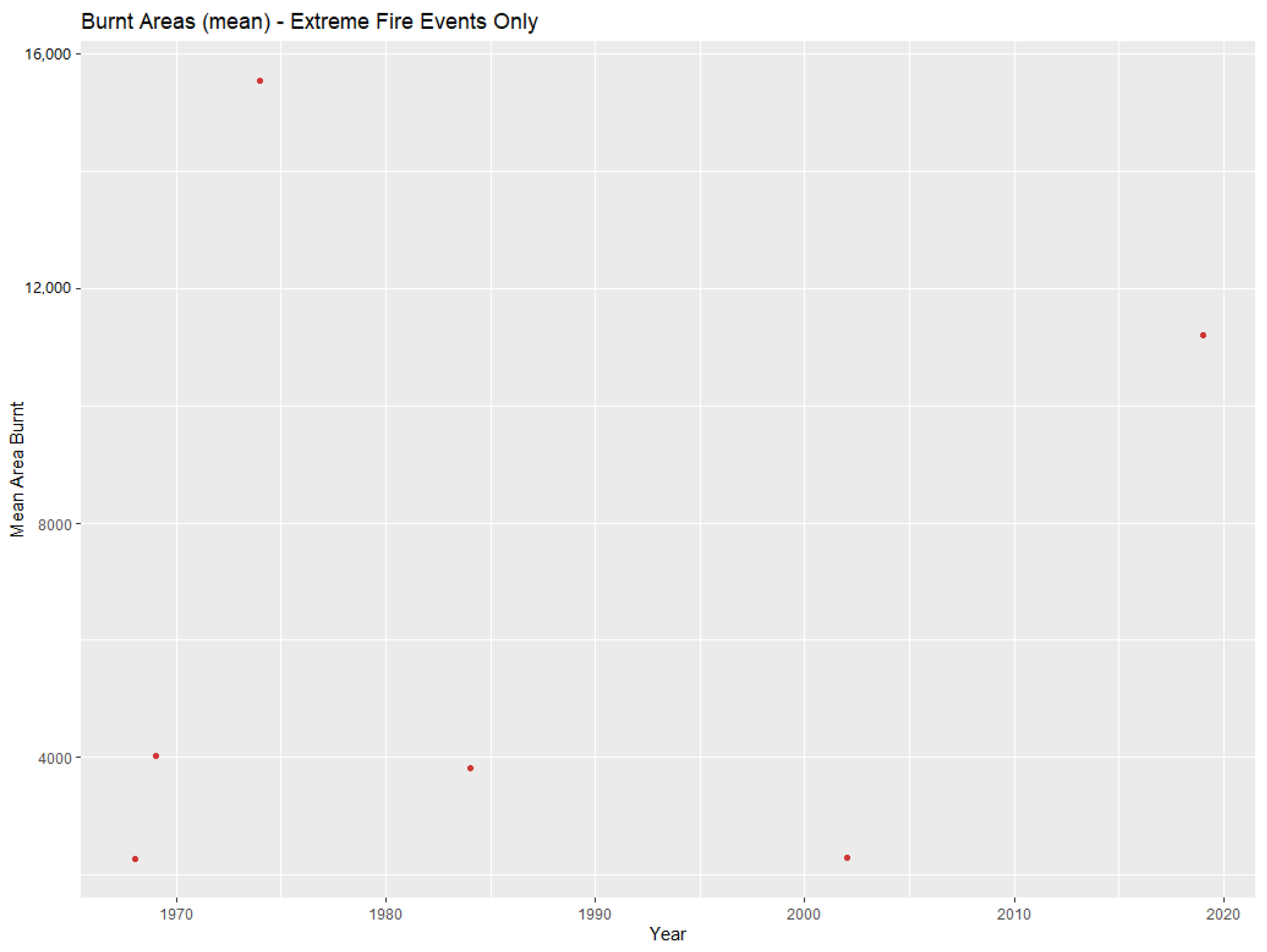
Figure 1. The NSW study area.
Buildings 11 00037 g001
Figure 2. The shapefile data and the attribute table of bushfire over 100 years, visualised in ArcGIS Pro.
Buildings 11 00037 g002
Figure 3. Snippet of R scripts for the linear modelling.
Buildings 11 00037 g003
Figure 4. Snippet of R scripts for the correlation method.
Buildings 11 00037 g004
Figure 5. Hotspot methodologies.
Buildings 11 00037 g005
Figure 6. A space-time cube.
Buildings 11 00037 g006
Figure 7. The geoprocessing model created with ArcGIS Pro’s ModelBuilder tool.
Buildings 11 00037 g007
Figure 8. The trend of areas burnt over time.
Buildings 11 00037 g008
Figure 9. Extreme fire events.
Buildings 11 00037 g009
Figure 10. Increase in the frequency of fires over time.
Buildings 11 00037 g010
Figure 11. Increase in the frequency of fires over time, split in two bins.
Buildings 11 00037 g011
Figure 12. Correlation between prescribed burns and bushfires.
Buildings 11 00037 g012
Figure 13. Hotspot analysis of the number of bushfires by statistical area level 2 in NSW.
Buildings 11 00037 g013
Figure 14. Bushfire frequency hotspot analysis in 2010–2020 by statistical area level 2 in NSW.
Buildings 11 00037 g014
Figure 15. Spatial patterns over time of bushfire frequency for each NSW statistical area level 2.
Buildings 11 00037 g015
Figure 16. Land-use types for the hotspots of fires.
Buildings 11 00037 g016
Figure 17. Bushfire frequency trends for each SA2.
Buildings 11 00037 g017
Figure 18. Snippet from the bushfire dashboard.
Buildings 11 00037 g018
Figure 19. The results section of the bushfire dashboard.
Buildings 11 00037 g019
Table 1. Statistical outliers.
SeasonMean Area Burnt (Hectares)
1974–197515,549
2019–2020 11,214
1969–19704027
1984–19853819
2002–20032296
1968–19692271
1977–19781887
Publisher’s Note: MDPI stays neutral with regard to jurisdictional claims in published maps and institutional affiliations.

