
An Exhaustive Search Energy Optimization Method for Residential Building Envelope in Different Climatic Zones of Kazakhstan


Abstract
:1. Introduction
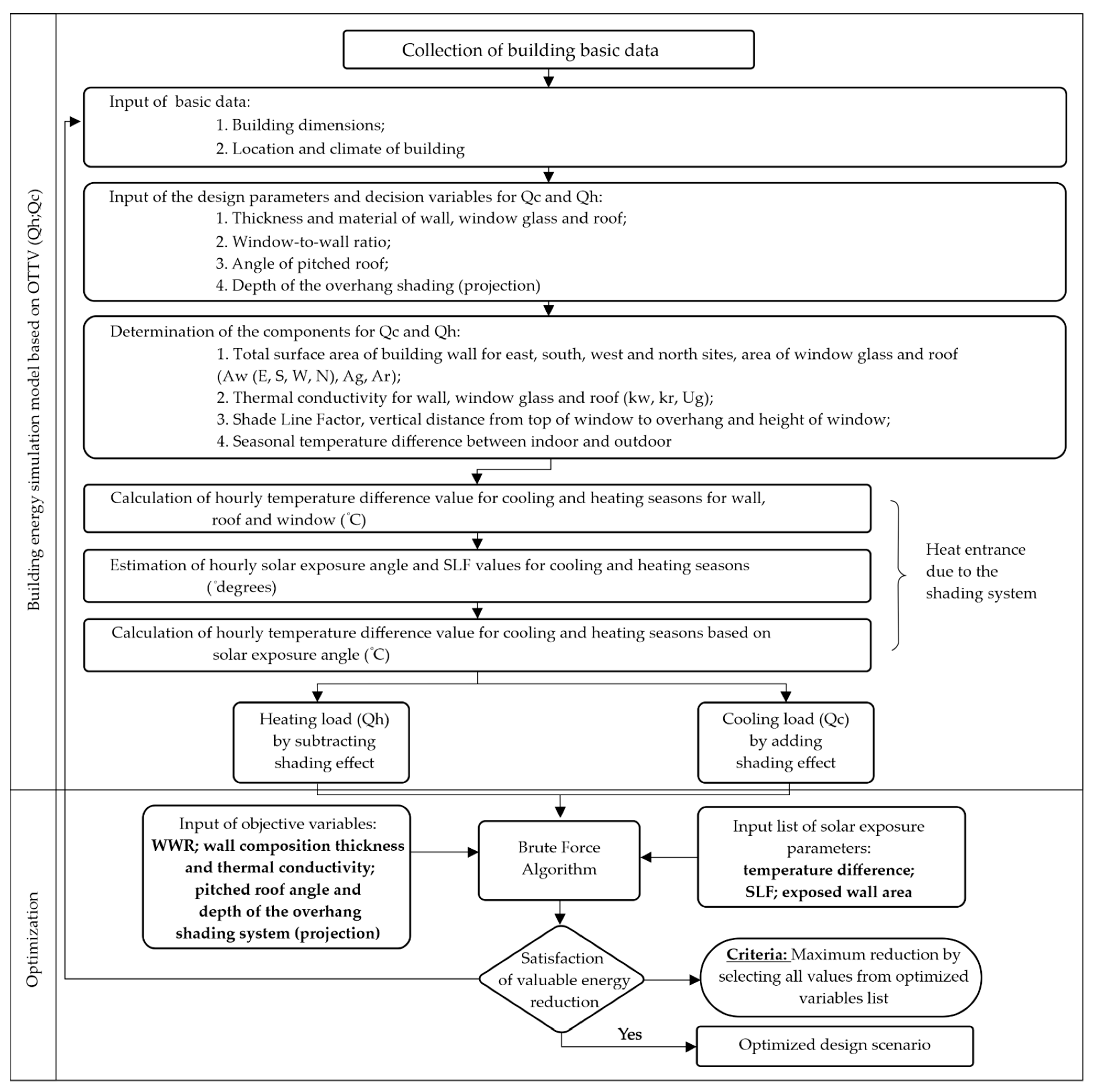
2. Methodology
2.1. The Overall Thermal Transfer Value (OTTV)
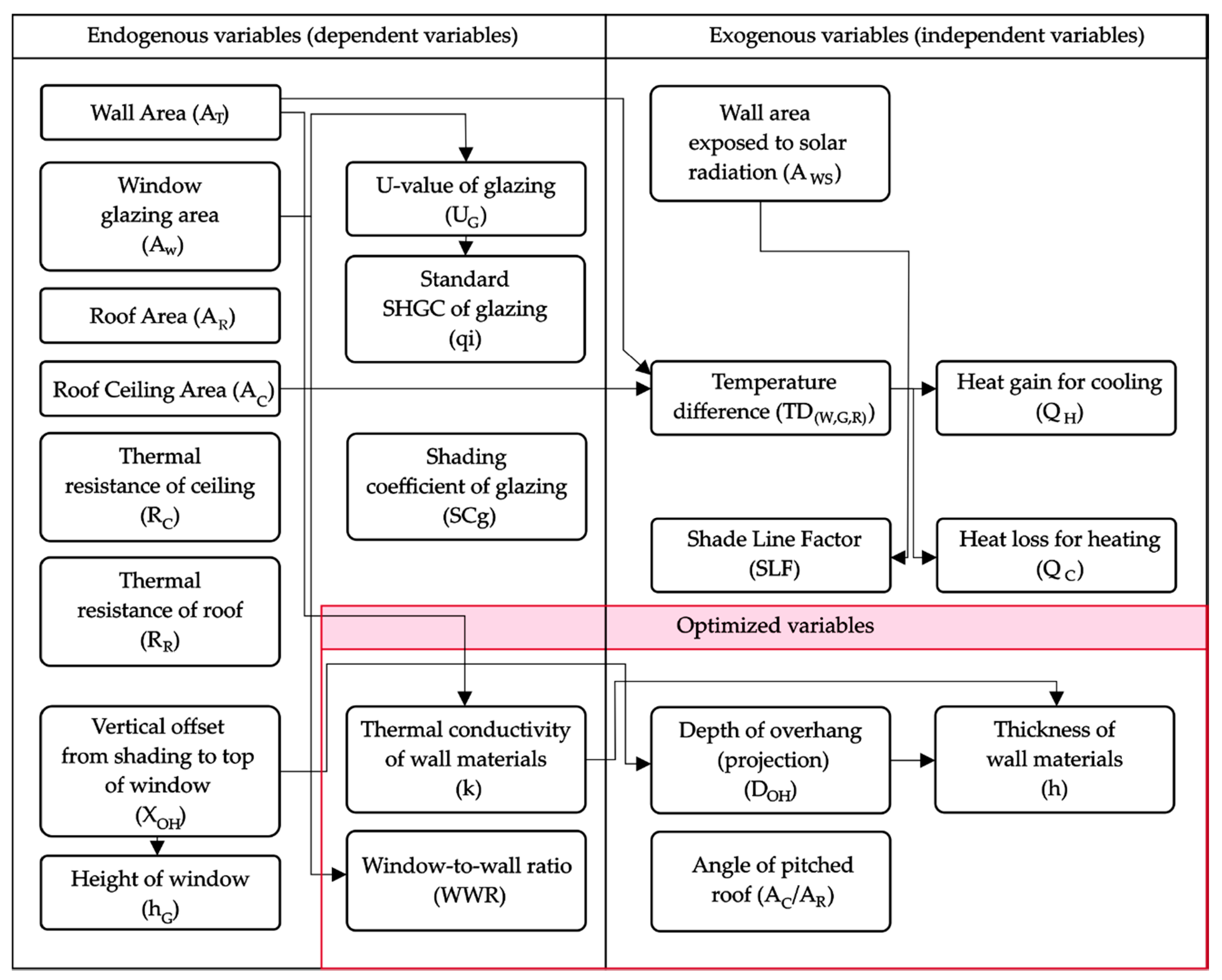
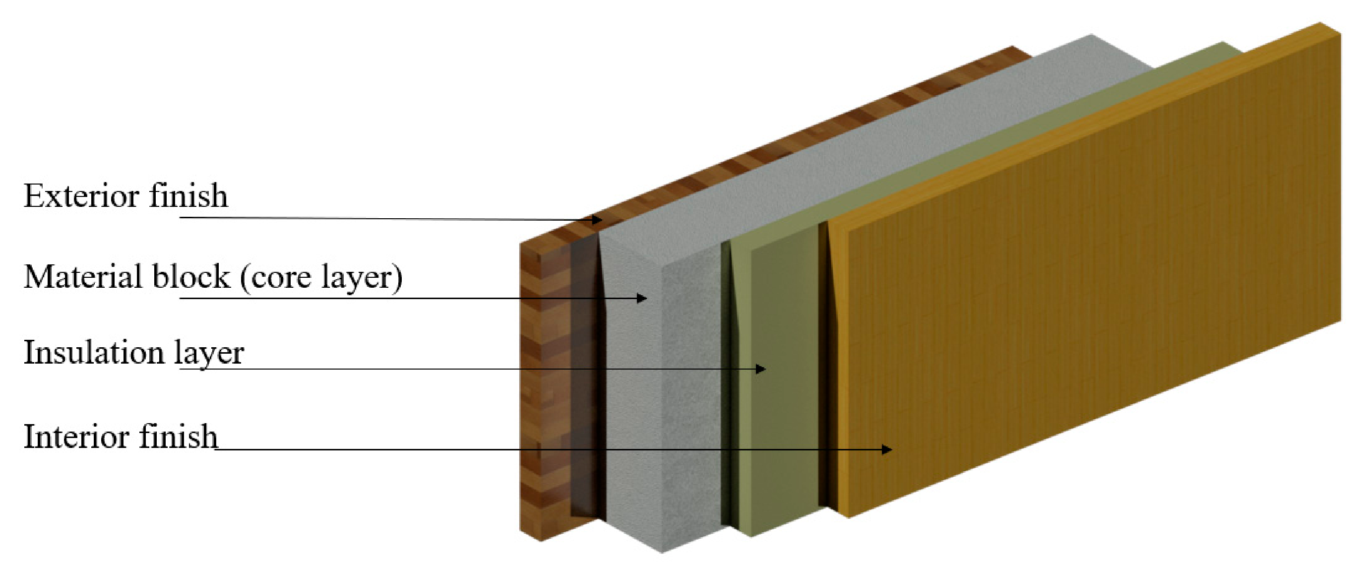
2.2. Building Envelope Parameters
Design Variables
2.3. Formulation of a Model
2.3.1. Heat Transfer through the Pitched Roof
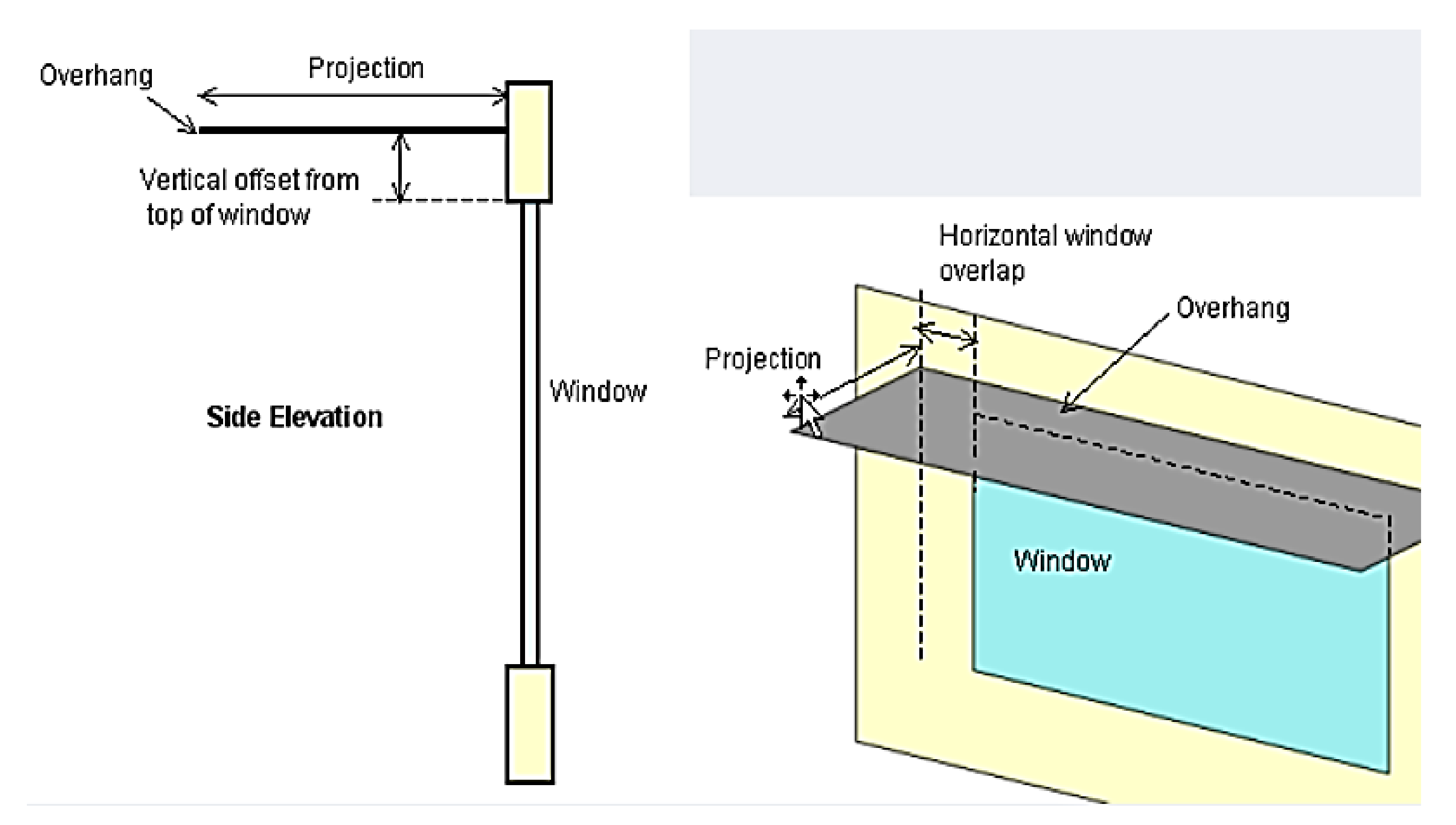
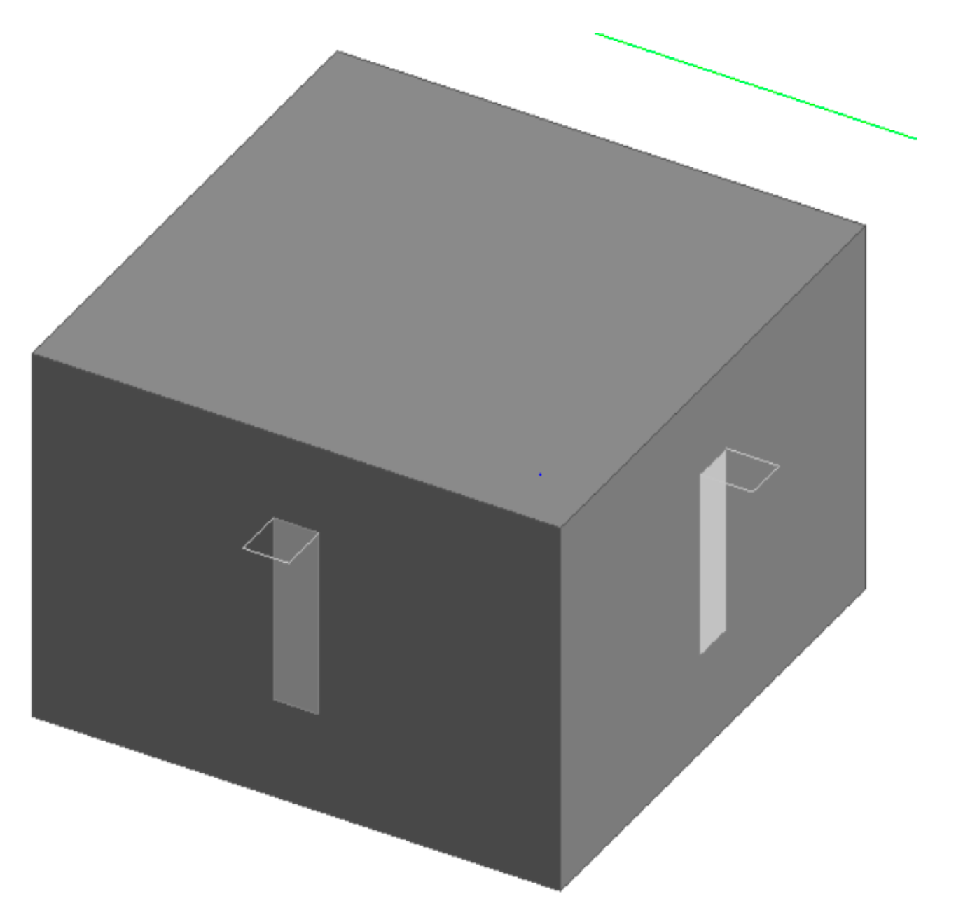
2.3.2. Details of Overhang Shading Device Configuration
- SC—total shading coefficient,
- SLF—shade line factor from [37],
- —depth of overhang (projection), m
- —vertical offset from the top of the window to overhang, m
- —height of the window, m.
2.4. Building Design Optimization
2.4.1. Optimization Variables
2.4.2. Optimization Algorithm
2.5. Verification of Results between Building Energy Simulation Model and DesignBuilder Software
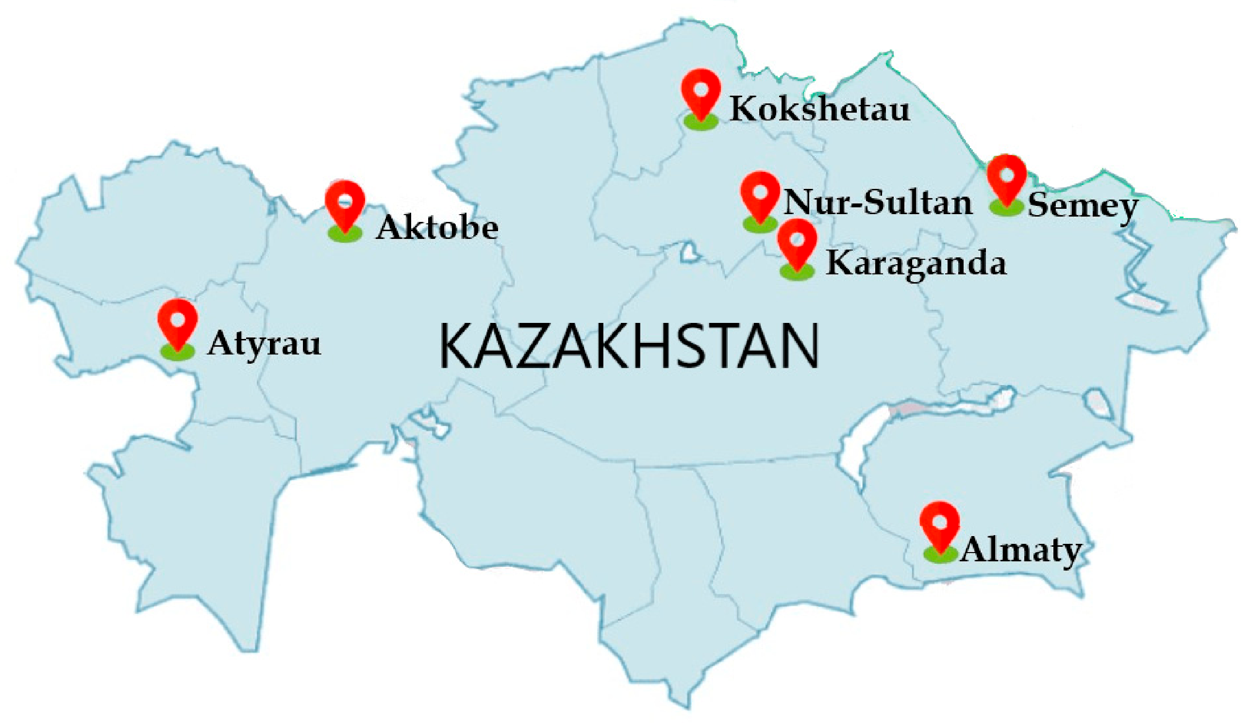
2.6. Case Study
2.6.1. Climate Conditions
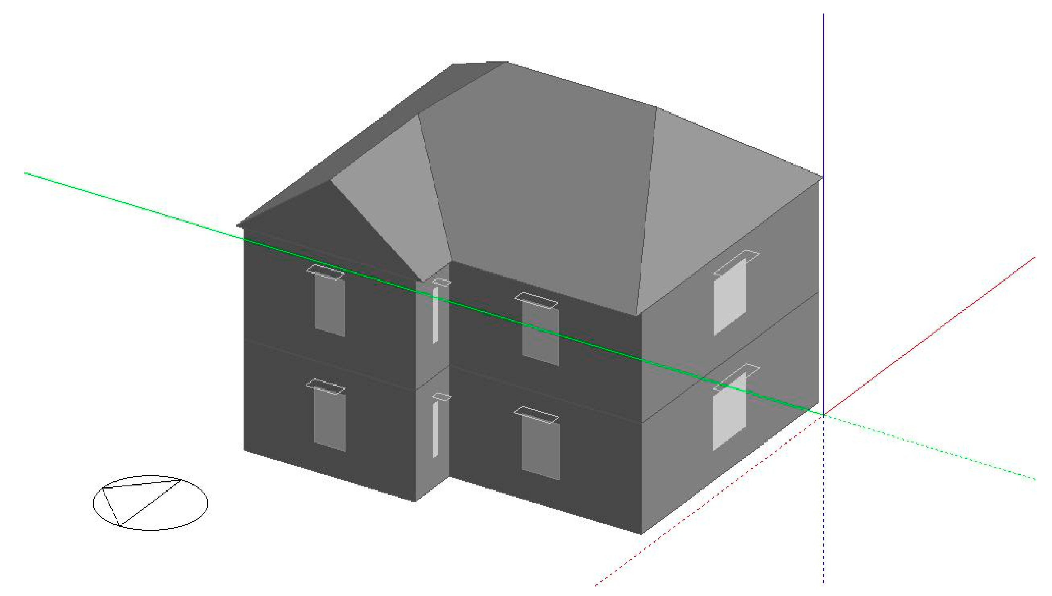
2.6.2. Building Model
3. Results and Discussion
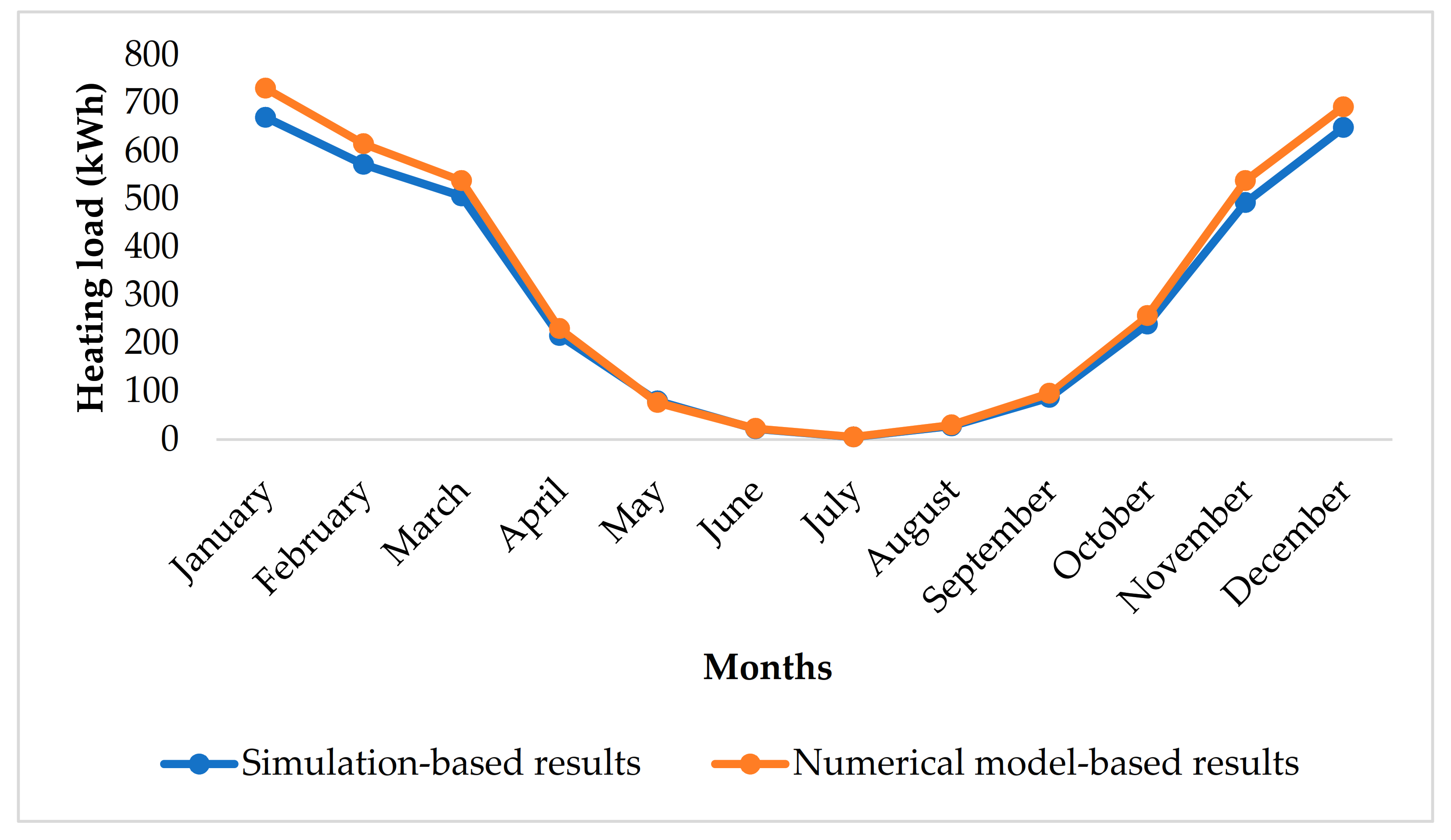
3.1. The Optimum Heating and Cooling Loads Reduction for Entire the Year

| Heating Load (kWh) | Heating Load | Cooling Load | Cooling Load | |||||
|---|---|---|---|---|---|---|---|---|
| List of Cities | Base Design | Optimized Design | Reduction in (kWh) | Reduction (Gcal) | Base Design | Optimized Design | Reduction in (kWh) | Reduction (Gcal) |
| Nur-Sultan | 41,848.71 | 34,905.05 | 6943.66 | 5.9701 | 11,538.66 | 9614.50 | 1924.16 | 1.6543 |
| Almaty | 28,673.86 | 23,915.51 | 4758.35 | 4.0912 | 13,453.56 | 11,345.62 | 2107.94 | 1.8124 |
| Karaganda | 40,564.44 | 33,833.53 | 6730.91 | 5.7872 | 12,280.95 | 10,233.19 | 2047.76 | 1.7606 |
| Aktobe | 38,536.64 | 32,142.22 | 6394.42 | 5.4979 | 9546.91 | 7955.13 | 1591.77 | 1.3686 |
| Atyrau | 30,500.17 | 25,439.52 | 5060.65 | 4.3511 | 12,213.90 | 10,179.55 | 2034.35 | 1.7491 |
| Semey | 37,651.78 | 31,402.88 | 6248.90 | 5.3728 | 10,304.82 | 8586.62 | 1718.19 | 1.4773 |
| Kokshetau | 41,996.78 | 35,028.89 | 6967.89 | 5.9909 | 11,759.43 | 9798.42 | 1961.01 | 1.6860 |
| Average: | 37,110.34 | 30,952.51 | 6157.82 | 5.2983 | 11,585.46 | 9673.29 | 1912.17 | 1.6453 |

| Envelope Components | Heating Energy Reduction (kWh) in Nur-Sultan | Heating Energy Reduction (kWh) in Koksetau | ||||
|---|---|---|---|---|---|---|
| Base Case | Optimized Case | Percentage of Contribution for Energy Reduction | Base Case | Optimized Case | Percentage of Contribution for Energy Reduction | |
| Wall | 16,095.01 | 13,410.52 | 6.37 | 16,156.16 | 13,461.60 | 6.38 |
| Window | 4067.69 | 3385.79 | 1.61 | 4069.49 | 3397.80 | 1.61 |
| Roof | 22,309.55 | 18,590.43 | 8.84 | 22,384.28 | 18,652.88 | 8.83 |
| Shading system | 523.11 | 624.80 | 0.30 | 524.96 | 630.52 | 0.30 |
| Total | 41,848.71 | 34,905.05 | 16.592 | 41,996.78 | 35,028.89 | 16.591 |
| Cooling Energy Reduction (kWh) in Almaty | Cooling Energy Reduction (kWh) in Atyrau | |||||
| Wall | 4802.92 | 4005.00 | 5.88 | 4702.35 | 3922.18 | 6.42 |
| Window | 1210.82 | 1008.63 | 1.48 | 1184.75 | 987.42 | 1.62 |
| Roof | 6713.33 | 5544.61 | 8.15 | 6143.59 | 5124.38 | 8.38 |
| Shading system | 980.76 | 816.88 | 1.20 | 549.63 | 458.08 | 0.75 |
| Total | 13,454 | 11,346 | 16.668 | 12,214 | 10,180 | 16.656 |
3.2. Economic Benefit of the Optimization
4. Conclusions
- This research has shown that proper selection of design variables can lead to notable energy savings in all cities. Due to the optimization of the numerical model analyzing the heat transfer through the envelope, the average annual heating reduction was 6156.8 kWh (or 5.29 Gcal), and the average cooling energy reduction was 1912.17 kWh (or 1.64 Gcal). In terms of percentage, heating and cooling energy were reduced by 16.59% and 16.69%, respectively. It is also concluded that the heating energy savings effect was more evident in the cities located in the northern part of Kazakstan (Nur-Sultan and Kokshetau), and the effect of the cooling energy savings was evident in the southern part (Almaty);
- Regarding monthly energy consumption, January, February, and December showed the highest energy consumption in each city. Overall energy consumption for heating and cooling throughout all months demonstrated that Kazakhstan’s climatic zone is mostly heating-dominated;
- The results showed that proper selection of orientation is critical. The direction of the frontage of the building towards the south in the cold season and north in the hot season showed around 21% and 32% energy reduction, respectively, which were effective compared with an initial orientation of the building;
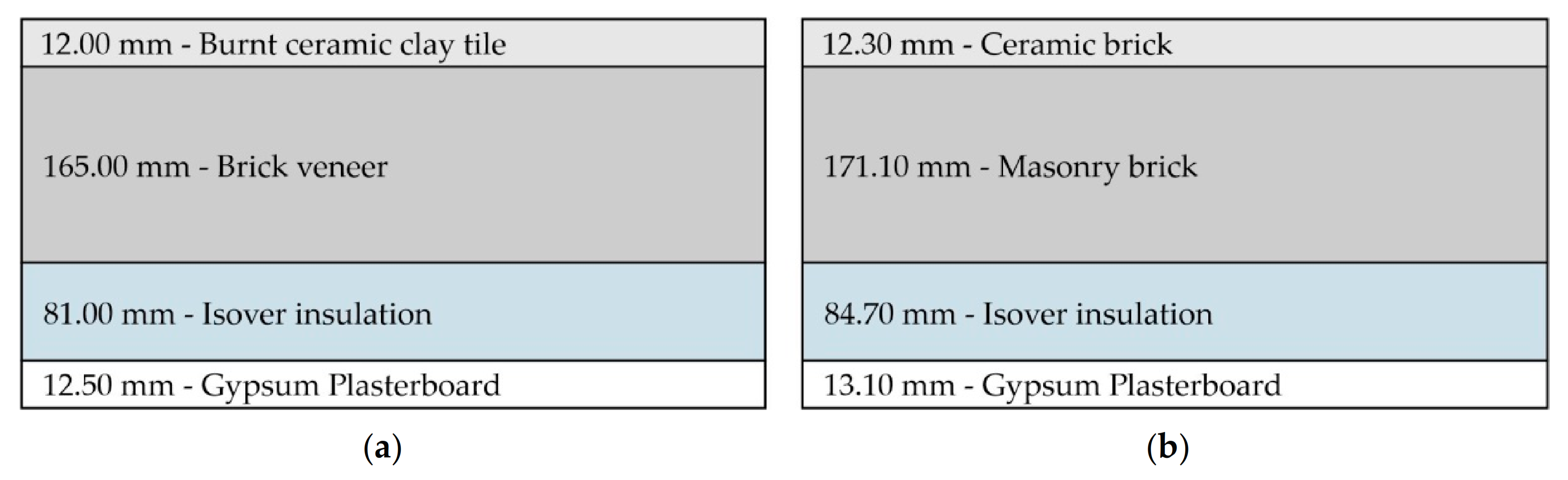
- The building orientation to the south, a combination of 0.7 m of the depth of the overhang shading system and the WWR of 4%, 12.30 mm ceramic brick as exterior finish, 171.10 mm masonry brick as core layer, 84.7 mm glasswool, and 13.10 mm plasterboard as the interior finish was found to be optimal design solution;
- From the economic analysis, it was found that equipment heating had a high-cost reduction compared to central heating. The highest cost reduction was observed in Atyrau with central heating and in Kokshetau with equipment-based heating, for cooling in Almaty. This highlights the fact that optimization of buildings brings significant economic benefits.
Author Contributions
Funding
Institutional Review Board Statement
Informed Consent Statement
Data Availability Statement
Conflicts of Interest
Abbreviations
| TDES | Total direct energy supply |
| TFEC | Total final energy consumption |
| PLA | Perimeter Annual Load |
| ENVLOAD | Envelope Energy Load |
| OTTV | Overall Thermal Transfer Value |
| TRNSYS | Transient System Simulation Tool |
| GMDH | Grouped Method of Data Handling type neural network |
| NSGA-II | Non-Dominated Sorting Genetic Algorithm II |
| ASHRAE | The American Society of Heating, Refrigerating and Air-Conditioning Engineers |
| HVAC | Heating, ventilation, and air conditioning |
| PCM | Phase change material |
| WNN | Wavelet neural network |
| MLP | Multi-Layer Perceptron neural network |
| ACO | Ant Colony Optimization |
| ABC | Artificial Bee Colony |
| PSO | Particle Swarm Optimization |
| BF | Brute force |
| BESM | Building Energy Simulation model |
| ETTV | Envelope Thermal Transfer Value |
| RTTV | Roof Transfer Value |
| SHGC | Standard solar heat gain coefficient of glazing |
| WWR | Window-to-wall ratio |
| Aw, Ag, Ar | Surface area of the wall, fenestration, and roof |
| kw | An overall thermal conductivity of the wall |
| kr | Thermal conductivity values of the roof |
| Ug | U-value of glazing |
| The exterior wall’s gross area | |
| Wall area exposed to solar radiation | |
| Heat gain through the envelope for the cooling season | |
| Heat loss through the envelope for the heating season | |
| Solar radiation through the fenestration | |
| h1, h2, h3, h4 | Thicknesses of wall composition layers |
| C1, C2, C3, C4 | Thermal conductivity values of wall composition layers |
| Thermal resistance value for roof ceiling | |
| Thermal resistance value for the roof | |
| Ceiling area | |
| Roof area | |
| Total area building’s wall | |
| SLF | Shade line factor |
| The depth of overhang (projection) | |
| Vertical offset from the top of the window to overhang | |
| The height of the window | |
| SCg | Shading coefficient of the glazing |
| SC | Total shading coefficient |
| α | The solar absorptivity constant related to the façade surface and color |
| TD | Equivalent temperature difference |
| TDw, TDr, TDg | Equivalent temperature differences between indoor and outdoor surrounding space wall, roof, and glazing |
| ESM | External shading multiplier |
| SF | Solar factor |
| q | The standard solar heat gain factor |
References
- Wang, X.; Zheng, H.; Wang, Z.; Shan, Y.; Meng, J.; Liang, X.; Feng, K.; Guan, D. Kazakhstan’s CO2 emissions in the post-Kyoto Protocol era: Production- and consumption-based analysis. J. Environ. Manag. 2019, 249, 109393. [Google Scholar] [CrossRef] [PubMed] [Green Version]
- Sarbassov, Y.; Kerimray, A.; Tokmurzin, D.; Tosato, G.; De Miglio, R. Electricity and heating system in Kazakhstan: Exploring energy efficiency improvement paths. Energy Policy 2013, 60, 431–444. [Google Scholar] [CrossRef]
- Assenova, B. What Is the Housing Stock in Kazakhstan—NewTimes.kz 2019. Available online: https://newtimes.kz/obshchestvo/96182-chto-iz-sebya-predstavlyaet-zhilishchnyj-fond-v-kazakhstane (accessed on 23 November 2021).
- History of Housing Construction in Kazakhstan. 2020. Available online: https://google-info.org/7523418/1/istoriya-zhilishchnogo-stroitelstva-v-kazakhstane.html (accessed on 24 November 2021).
- Agency for Strategic Planning and Reforms of the Republic of Kazakhstan Bureau of National Statistics n.d. Available online: https://stat.gov.kz/search (accessed on 24 November 2021).
- Energy-Efficient Design and Construction of Residential Buildings. United Nations, Development Programme, PIMS No. 4133 Atlas Award 00059795, Project ID 0074950. Available online: https://www.kz.undp.org/content/kazakhstan/en/home/operations/projects/environment_and_energy/energy-efficient-design-and-construction-of-residential-building.html (accessed on 27 November 2021).
- Imani, N.; Vale, B. A framework for finding inspiration in nature: Biomimetic energy efficient building design. Energy Build. 2020, 225, 110296. [Google Scholar] [CrossRef]
- Yu, J.; Yang, C.; Tian, L.; Liao, D. Evaluation on energy and thermal performance for residential envelopes in hot summer and cold winter zone of China. Appl. Energy 2009, 86, 1970–1985. [Google Scholar] [CrossRef]
- Huang, J.; Deringer, J. Status of Energy Efficient Building Codes in Asia; The Asia Business Council: Hong Kong, China, 2017; pp. 6–9. [Google Scholar]
- Lin, Y.-H.; Tsai, K.-T.; Lin, M.-D.; Yang, M.-D. Design optimization of office building envelope configurations for energy conservation. Appl. Energy 2016, 171, 336–346. [Google Scholar] [CrossRef]
- Yang, K.; Hwang, R.-L. Energy conservation of buildings in Taiwan. Pattern Recognit. 1995, 28, 1483–1491. [Google Scholar] [CrossRef]
- Yang, K.H.; Hwang, R.L. The analysis of design strategies on building energy conservation in Taiwan. Build. Environ. 1993, 28, 429–438. [Google Scholar] [CrossRef]
- Yang, K.-H.; Hwang, R.-L. An improved assessment model of variable frequency-driven direct expansion air-conditioning system in commercial buildings for Taiwan green building rating system. Build. Environ. 2007, 42, 3582–3588. [Google Scholar] [CrossRef]
- Huang, K.T.; Lin, H.T. Design standard of energy conservation for building hvac system—A simplified method of chiller capacity estimation based on building envelope energy conservation index in taiwan. In Proceedings of the IBPSA 2005—International Building Performance Simulation Association 2005, Montréal, QC, Canada, 15–18 August 2005; pp. 435–442. [Google Scholar]
- Chan, A.; Chow, T. Calculation of overall thermal transfer value (OTTV) for commercial buildings constructed with naturally ventilated double skin façade in subtropical Hong Kong. Energy Build. 2014, 69, 14–21. [Google Scholar] [CrossRef]
- Guo, J.; Hermelin, D.; Komusiewicz, C. Local search for string problems: Brute-force is essentially optimal. Theor. Comput. Sci. 2014, 525, 30–41. [Google Scholar] [CrossRef]
- Robinson, A.C.; Quinn, S.D. A brute force method for spatially-enhanced multivariate facet analysis. Comput. Environ. Urban Syst. 2018, 69, 28–38. [Google Scholar] [CrossRef]
- Al-Saadi, S.N.J.; Al-Jabri, K.S. Energy-efficient envelope design for residential buildings: A case study in Oman. In Proceedings of the 2017 Smart Cities Symp Prague, SCSP 2017—IEEE Proceedings 2017, Prague, Czech Republic, 25–26 May 2017. [Google Scholar] [CrossRef]
- Hui Sam, C.M. Overall thermal transfer value (OTTV): How to improve its control in Hong Kong. In Proceedings of the One-day Symposium on Building, Energy and Environment, Hong Kong, China, 16 October 1997; Volume 16, pp. 12-1–12-11. [Google Scholar]
- Devgan, S.; Jain, A.; Bhattacharjee, B. Predetermined overall thermal transfer value coefficients for Composite, Hot-Dry and Warm-Humid climates. Energy Build. 2010, 42, 1841–1861. [Google Scholar] [CrossRef]
- Chan, L.S. Investigating the thermal performance and Overall Thermal Transfer Value (OTTV) of air-conditioned buildings under the effect of adjacent shading against solar radiation. J. Build. Eng. 2021, 44, 103211. [Google Scholar] [CrossRef]
- Chou, S.K.; Chang, W.L. Development of an energy-estimating equation for large commercial buildings. Int. J. Energy Res. 1993, 17, 759–773. [Google Scholar] [CrossRef]
- Djamila, H.; Rajin, M.; Rizalman, A.N. Energy efficiency through building envelope in Malaysia and Singapore. J. Adv. Res. Fluid Mech. Therm. Sci. 2018, 46, 96–105. [Google Scholar]
- Zhang, Y.; Long, E.; Li, Y.; Li, P. Solar radiation reflective coating material on building envelopes: Heat transfer analysis and cooling energy saving. Energy Explor. Exploit. 2017, 35, 748–766. [Google Scholar] [CrossRef] [Green Version]
- Mustafaraj, G.; Marini, D.; Costa, A.; Keane, M. Model calibration for building energy efficiency simulation. Appl. Energy 2014, 130, 72–85. [Google Scholar] [CrossRef]
- Kutlu, L.; Tran, K.C.; Tsionas, M.G. A spatial stochastic frontier model with endogenous frontier and environmental variables. Eur. J. Oper. Res. 2020, 286, 389–399. [Google Scholar] [CrossRef]
- Lleras, C. Path Analysis. Encycl. Soc. Meas. 2005, 3, 25–30. [Google Scholar] [CrossRef]
- Zhang, Y.; Sun, X.; Medina, M.A. Calculation of transient phase change heat transfer through building envelopes: An improved enthalpy model and error analysis. Energy Build. 2020, 209, 109673. [Google Scholar] [CrossRef]
- White Box Technologies Weather Data, n.d. Available online: http://weather.whiteboxtechnologies.com/ (accessed on 24 November 2021).
- Xing, F.; Mohotti, D.; Chauhan, K. Study on localised wind pressure development in gable roof buildings having different roof pitches with experiments, RANS and LES simulation models. Build. Environ. 2018, 143, 240–257. [Google Scholar] [CrossRef]
- Çengel, Y.; Ghajar, R.A. Heat and Mass Transfer: Fundamentals & Applications. 2015. Available online: https://studylib.net/doc/8394668/heating-and-cooling-of-buildings (accessed on 8 December 2021).
- Shen, H.; Tzempelikos, A. Daylighting and energy analysis of private offices with automated interior roller shades. Sol. Energy 2012, 86, 681–704. [Google Scholar] [CrossRef]
- Barnaby, C.S.; Wright, J.L.; Collins, M.R. Improving load calculations for fenestration with shading devices. ASHRAE Trans. 2009, 115, 31–44. [Google Scholar]
- Kotey, N.A.; Wright, J.L.; Barnaby, C.S.; Collins, M.R. Solar gain through windows with shading devices: Simulation versus measurement. ASHRAE Trans. 2009, 115, 18–30. [Google Scholar]
- Bessoudo, M.; Tzempelikos, A.; Athienitis, A.; Zmeureanu, R. Indoor thermal environmental conditions near glazed facades with shading devices—Part I: Experiments and building thermal model. Build. Environ. 2010, 45, 2506–2516. [Google Scholar] [CrossRef]
- DesignBuilder Software Ltd.—Previous Versions n.d. Available online: https://designbuilder.co.uk/download/previous-versions (accessed on 22 October 2021).
- Residential Cooling and Heating Load Calculations. In ASHRAE Handbook of Fundamentals; SI Edition; ASHRAE: Atlanta, GA, USA, 2017; Chapter 17.
- Ozmen, Y.; Baydar, E.; van Beeck, J. Wind flow over the low-rise building models with gabled roofs having different pitch angles. Build. Environ. 2016, 95, 63–74. [Google Scholar] [CrossRef]
- Szcześniak, J.T.; Ang, Y.Q.; Letellier-Duchesne, S.; Reinhart, C.F. A method for using street view imagery to auto-extract window-to-wall ratios and its relevance for urban-level daylighting and energy simulations. Build. Environ. 2021, 2021, 108108. [Google Scholar] [CrossRef]
- Xue, P.; Li, Q.; Xie, J.; Zhao, M.; Liu, J. Optimization of window-to-wall ratio with sunshades in China low latitude region considering daylighting and energy saving requirements. Appl. Energy 2019, 233–234, 62–70. [Google Scholar] [CrossRef]
- GOST 530-2012. Interstate Standard. Ceramic Brick and Stone. General Specifications. 2012. Available online: https://docs.cntd.ru/document/1200100260 (accessed on 27 November 2021).
- GOST 9573-2012. Interstate Standard. Thermal Insulating Plates of Mineral Wool on Syntetic Binder. Specifications. 2013, pp. 14–27. Available online: https://docs.cntd.ru/document/1200101613 (accessed on 27 November 2021).
- SN RK 2.04-04-2011. State Standards in the Field of Architecture, Urban Planning and Construction. Thermal Protection of Buildings. 2011. Available online: http://www.hoffmann.kz/files/12_SN_RK_2-04-04-2011.pdf (accessed on 27 November 2021).
- GOST 24992-81. State Standard of the Union of SSR. Masonary Structures. Method of Estimating Bonding Strength in Masonry. 1995. Available online: http://gostrf.com/normadata/1/4294853/4294853407.html (accessed on 27 November 2021).
- GOST 31310-2015. Interstate Standard. Wall Three-Layer Reinforced Concrete Panels with Enerqy-Efficient Insulation. General Specifications. Interstate Council for Standardization, Metrology and Certification (isc). 2017. Available online: https://docs.cntd.ru/document/1200133283 (accessed on 27 November 2021).
- Peel, M.C.; Finlayson, B.L.; McMahon, T.A. Updated world map of the Köppen-Geiger climate classification. Hydrol. Earth Syst. Sci. 2007, 11, 1633–1644. [Google Scholar] [CrossRef] [Green Version]
- Climate Data for Cities Worldwide—Climate-Data.org n.d. Available online: https://en.climate-data.org/ (accessed on 22 October 2021).
- Mutschler, R.; Rüdisüli, M.; Heer, P.; Eggimann, S. Benchmarking cooling and heating energy demands considering climate change, population growth and cooling device uptake. Appl. Energy 2021, 288, 116636. [Google Scholar] [CrossRef]
- Tootkaboni, M.P.; Ballarini, I.; Corrado, V. Analysing the future energy performance of residential buildings in the most populated Italian climatic zone: A study of climate change impacts. Energy Rep. 2021, 7, 8548–8560. [Google Scholar] [CrossRef]
- Albatayneh, A. Optimising the Parameters of a Building Envelope in the East Mediterranean Saharan, Cool Climate Zone. Buildings 2021, 11, 43. [Google Scholar] [CrossRef]
- Alshboul, A.A.; Alkurdi, N.Y. Enhancing the Strategies of Climate Responsive Architecture, The Study of Solar Accessibility for Buildings Standing on Sloped Sites. Mod. Appl. Sci. 2018, 13, 69. [Google Scholar] [CrossRef] [Green Version]


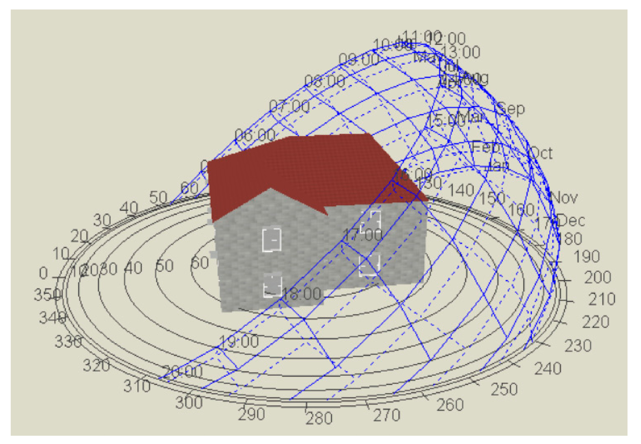
| 1st of January (Time) | Exposure Site | Angle of Sunlight (°) |
|---|---|---|
| 9:00 | southeast | 4.73 |
| 10:00 | southeast | 10.82 |
| 11:00 | southeast | 15.15 |
| 12:00 | southeast | 17.45 |
| 13:00 | southwest | 17.39 |
| 14:00 | southwest | 14.99 |
| 15:00 | southwest | 10.4 |
| 16:00 | southwest | 3.08 |
| Layers | Materials | Thickness, (h1, h2, h3, h4), (m) | Thermal Conductivity, (C1, C2, C3, C4), (W/mK) | Density | Specific Heat (J/kgK) |
|---|---|---|---|---|---|
| Exterior finish | Ceramic brick | 0.5 | 0.59 | 1831 | 825 |
| Cement sand render | 0.02 | 1 | 1800 | 1000 | |
| Limestone mortar | 0.02 | 0.7 | 1600 | 840 | |
| Burnt ceramic clay tile | 0.012 | 1.3 | 2000 | 840 | |
| Dry ceramic clay tile | 0.012 | 1.2 | 2000 | 850 | |
| Clay block | 0.0075 | 1.4 | 2500 | 840 | |
| Material Block (Core layer) | Masonry block | 0.15 | 0.24 | 800 | 840 |
| Burnt brick veneer | 0.15 | 0.74 | 1700 | 800 | |
| Aerated concrete block | 0.2 | 0.24 | 750 | 1000 | |
| Brick veneer | 0.15 | 0.547 | 1950 | 1000 | |
| Reinforced concrete | 0.15 | 0.5 | 1400 | 830 | |
| Clay block | 0.19 | 1.0 | 1800 | 920 | |
| Insulation layer | Penoplex | 0.0795 | 0.030 | 30 | 1340 |
| Glasswool | 0.012 | 0.039 | 20 | 840 | |
| Hydro isolation | 0.015 | 0.29 | 29 | 1210 | |
| Mineral wool plate | 0.1 | 0.036 | 70 | 810 | |
| Extruded polystyrene | 0.0795 | 0.03 | 43 | 1210 | |
| Cellulose | 0.2 | 0.04 | 48 | 1381 | |
| Interior finish | Gypsum Board | 0.013 | 0.16 | 800 | 1090 |
| Cement mortar | 0.012 | 0.72 | 1760 | 840 | |
| Gypsum insulating plaster | 0.013 | 0.18 | 600 | 1000 | |
| Plaster board 1 | 0.012 | 0.72 | 840 | 1860 | |
| Plaster board 2 | 0.012 | 0.25 | 600 | 1089 | |
| Plaster board 3 | 0.012 | 0.35 | 817 | 1620 |
| 1-st of January | Temperature Difference (°C) | Shade Line Factor | Wall Area Exposed to Solar Radiation (m2) |
|---|---|---|---|
| 9:00 | 37.58 | 2.43 | 144 |
| 10:00 | 36.98 | 2.29 | 144 |
| 11:00 | 36.2 | 2.18 | 144 |
| 12:00 | 35.4 | 2.13 | 144 |
| 13:00 | 34.6 | 2.13 | 156 |
| 14:00 | 33.88 | 2.19 | 156 |
| 15:00 | 33.4 | 2.30 | 156 |
| 16:00 | 33.53 | 2.47 | 156 |
| Composition Materials | Layers | Material | Thickness, (h1, h2, h3, h4), (m) | Thermal Conductivity, (C1, C2, C3, C4), (W/mK) | Density | Specific Heat (J/kgK) |
|---|---|---|---|---|---|---|
| Wall | Exterior finish | Burnt ceramic clay tile | 0.012 | 1.3 | 2000 | 840 |
| Core layer | Brick veneer | 0.0165 | 0.542 | 1950 | 840 | |
| Insulation | Glasswool | 0.081 | 0.039 | 20 | 840 | |
| Interior finish | Plaster board | 0.0125 | 0.35 | 817 | 1620 | |
| Roof | Exterior finish | Roof tile | 0.01 | 0.84 | 1900 | 800 |
| Core layer | Concrete slab | 0.15 | 1.13 | 2000 | 1000 | |
| Insulation | Polystyrene | 0.2423 | 0.29 | 29 | 1210 | |
| Interior finish | Roofing felt | 0.005 | 0.19 | 960 | 837 |
| City | Latitude | Longitude | Climate Zone (According to Koppen Classification) | The Average Temperature in January (°C) | The Average Temperature in July (°C) |
|---|---|---|---|---|---|
| Nur-Sultan | 51.18 | 71.45 | Dfb | −18.3 | 20 |
| Almaty | 43.25 | 76.92 | Dfa | −8.4 | 24 |
| Karaganda | 49.83 | 73.16 | Dfb | −14.2 | 18 |
| Aktobe | 43.25 | 67.76 | Dfa | −16.5 | 25 |
| Atyrau | 47.11 | 51.88 | Bwk | −9.9 | 27 |
| Semey | 50.41 | 80.20 | Dfb | −12.2 | 18 |
| Kokshetau | 53.28 | 69.39 | Bsk | −19.7 | 20 |
| Nur-Sultan | Almaty | Aktobe | Atyrau | Karaganda | Semey | Kokshetau | ||||||||
|---|---|---|---|---|---|---|---|---|---|---|---|---|---|---|
| Months | Base | Optimized | Base | Optimized | Base | Optimized | Base | Optimized | Base | Optimized | Base | Optimized | Base | Optimized |
| January | 10,009 | 8349 | 6858 | 5720 | 9217 | 7688 | 7295 | 6085 | 9702 | 8092 | 9006 | 7511 | 10,045 | 8378 |
| February | 7436 | 6202 | 5095 | 4249 | 6847 | 5711 | 5419 | 4520 | 7207 | 6011 | 6690 | 5580 | 7462 | 6224 |
| March | 4671 | 3896 | 3200 | 2669 | 4301 | 3588 | 3404 | 2839 | 4528 | 3776 | 4203 | 3505 | 4688 | 3910 |
| April | 3050 | 2544 | 2090 | 1743 | 2809 | 2343 | 2223 | 1854 | 2957 | 2466 | 2745 | 2289 | 3061 | 2553 |
| May | 1239 | 1034 | 849 | 708 | 1141 | 952 | 903 | 753 | 1201 | 1002 | 1115 | 930 | 1244 | 1037 |
| June | 1846 | 1538 | 1119 | 932 | 1528 | 1273 | 1954 | 1629 | 1965 | 1637 | 1649 | 1374 | 1882 | 1568 |
| July | 4846 | 4038 | 2936 | 2447 | 4010 | 3341 | 5130 | 4275 | 5158 | 4298 | 4328 | 3606 | 4939 | 4115 |
| August | 4269 | 3557 | 2587 | 2156 | 3532 | 2943 | 4519 | 3766 | 4544 | 3786 | 3813 | 3177 | 4351 | 3625 |
| September | 577 | 481 | 350 | 291 | 477 | 398 | 611 | 509 | 614 | 512 | 515 | 429 | 588 | 490 |
| October | 2574 | 2147 | 1764 | 1471 | 2370 | 1977 | 1876 | 1565 | 2495 | 2081 | 2316 | 1931 | 2583 | 2154 |
| November | 4957 | 4135 | 3396 | 2833 | 4565 | 3807 | 3613 | 3013 | 4805 | 4008 | 4460 | 3720 | 4975 | 4149 |
| December | 7912 | 6599 | 5421 | 4522 | 7286 | 6077 | 5767 | 4810 | 7669 | 6397 | 7119 | 5937 | 7940 | 6623 |
| List of Cities | Heating (kWh) | Cooling (kWh) | ||||||||
|---|---|---|---|---|---|---|---|---|---|---|
| Base Design | Optimized Design | Base Design | Optimized Design | |||||||
| West | North | East | South | West | North | East | South | |||
| Nur-Sultan | 41,848.71 | 34,905.05 | 33,405.05 | 36,405.05 | 33,205.05 | 11,538.66 | 9614.50 | 7914.50 | 11,114.50 | 8114.50 |
| Almaty | 28,673.86 | 23,915.51 | 22,415.51 | 25,415.51 | 22,215.51 | 13,453.56 | 5825.71 | 4125.71 | 7325.71 | 4325.71 |
| Aktobe | 38,536.64 | 32,142.22 | 30,642.22 | 33,642.22 | 30,442.22 | 9546.91 | 7955.13 | 6255.13 | 9455.13 | 6455.13 |
| Karaganda | 40,564.44 | 33,833.53 | 32,333.53 | 35,333.53 | 32,133.53 | 12,280.95 | 10,233.19 | 8533.19 | 11,733.19 | 8733.19 |
| Atyrau | 30,500.17 | 25,439.52 | 23,939.52 | 26,939.52 | 23,739.52 | 12,213.90 | 10,179.55 | 8479.55 | 11,679.55 | 8679.55 |
| Kokshetau | 41,996.78 | 35,028.89 | 33,528.89 | 36,528.89 | 33,328.89 | 11,759.43 | 9798.42 | 8098.42 | 11,298.42 | 8298.42 |
| Semey | 37,651.78 | 31,402.88 | 29,902.88 | 32,902.88 | 29,702.88 | 10,304.82 | 8586.62 | 6886.62 | 10,086.62 | 7086.62 |
| Heating Energy Reduction | ||||||
|---|---|---|---|---|---|---|
| List of Cities | Energy Reduction (kWh) | Energy Reduction (Gcal) | Price Rate (₸ per Gcal) | Price Rate (₸ per kWh) | Economic Impact (₸ for the Period) | |
| Centralized Heating | Equipment Heating | |||||
| Nur-Sultan | 6943.66 | 5.97 | 2176.76 | 11.93 | 12,996 | 82,838 |
| Almaty | 4758.35 | 4.09 | 4881.79 | 17.12 | 19,973 | 81,463 |
| Karaganda | 6394.42 | 5.49 | 2758.57 | 8.75 | 15,166 | 55,951 |
| Aktobe | 6730.91 | 5.79 | 3042.32 | 10.02 | 17,607 | 67,444 |
| Atyrau | 5060.65 | 4.35 | 4832.88 | 4.73 | 21,029 | 23,937 |
| Semey | 6967.89 | 5.99 | 1611.98 | 17.11 | 9657 | 119,221 |
| Kokshetau | 6248.90 | 5.37 | 3018.12 | 10.395 | 16,216 | 64,957 |
| Cooling Energy Reduction | ||||||
| Nur-Sultan | 1924.16 | 1.65 | 11.93 | 22,955 | ||
| Almaty | 2107.94 | 1.81 | 17.12 | 36,088 | ||
| Karaganda | 2047.77 | 1.76 | 10.02 | 20,519 | ||
| Aktobe | 1591.77 | 1.36 | 8.75 | 13,928 | ||
| Atyrau | 2034.35 | 1.74 | 4.73 | 9622 | ||
| Semey | 1718.19 | 1.47 | 10.395 | 17,861 | ||
| Kokshetau | 1961.00 | 1.68 | 17.11 | 33,553 | ||
Publisher’s Note: MDPI stays neutral with regard to jurisdictional claims in published maps and institutional affiliations. |
© 2021 by the authors. Licensee MDPI, Basel, Switzerland. This article is an open access article distributed under the terms and conditions of the Creative Commons Attribution (CC BY) license (https://creativecommons.org/licenses/by/4.0/).
Share and Cite
Kaderzhanov, M.; Memon, S.A.; Saurbayeva, A.; Kim, J.R. An Exhaustive Search Energy Optimization Method for Residential Building Envelope in Different Climatic Zones of Kazakhstan. Buildings 2021, 11, 633. https://doi.org/10.3390/buildings11120633
Kaderzhanov M, Memon SA, Saurbayeva A, Kim JR. An Exhaustive Search Energy Optimization Method for Residential Building Envelope in Different Climatic Zones of Kazakhstan. Buildings. 2021; 11(12):633. https://doi.org/10.3390/buildings11120633
Chicago/Turabian StyleKaderzhanov, Mirzhan, Shazim Ali Memon, Assemgul Saurbayeva, and Jong R. Kim. 2021. "An Exhaustive Search Energy Optimization Method for Residential Building Envelope in Different Climatic Zones of Kazakhstan" Buildings 11, no. 12: 633. https://doi.org/10.3390/buildings11120633